考量管線時間之延伸指令集

全文

(1)國立交通大學資訊科學與工程研究所碩士論文考量管線時間之延伸指令集. Instruction Set Extension with Consideration of Pipestage Timing. 研究生：黃士嘉指導教授：鍾崇斌. 教授. 中華民國九十五年七月.

(2) 考量管線時間之延伸指令集 Instruction Set Extension with Consideration of Pipestage Timing 研究生：黃士嘉. Student：Shih-Chia Huang. 指導教授：鍾崇斌. Advisor：Chung-Ping Chung. 國立交通大學資訊科學與工程研究所碩士論文. A Thesis Submitted to Institute of Computer Science and Engineering College of Computer Science National Chiao Tung University in partial Fulfillment of the Requirements for the Degree of Master in Computer Science July 2006 Hsinchu, Taiwan, Republic of China. 中華民國九十五年七月 1.

(3) 考量管線時間之延伸指令集學生：黃士嘉. 指導教授：鍾崇斌. 教授. 國立交通大學資訊科學與工程研究所碩士班. 摘要延伸指令集(ISE)是一種有效的方式可以滿足在許多應用上不斷增加的電路以及速度的需求。ISE 產生的流程通常包含了 ISE Exploration 以及 ISE Selection 兩個步驟，在 ISE Exploration 的步驟中，為了要達到最高的加速效果，大多數的研究都直接使用速度最快的實做方式來實做每一個在特殊的功能單元(ASFU)中的基本運算，而 ASFU 也就是複雜執行延伸指令集的功能單元，儘管如此，最快速的實作方式卻不一定是最好的選擇，在選擇 ASFU 中的運算的實作方式時，有兩點重要的考量：(1)ASFU 的執行時間必須符合管線時間的限制，也就是必須與原本管線時脈的整數倍相同，並且在(1)的前提下，(2)ASFU 必須使用最少的額外面積，為了要滿足這些考量，我們提出了一個 ISE Exploration 的演算法不只可以探索 ISE 候選者，也同時考慮了它們的實作方式以期能夠減少最多的執行時間，並且在此同時使用較少的面積。使用 Mibench 的模擬結果顯示，與沒有考量管線時間的 ASFU 比較，這個方法可以額外節省 35.28%、15.92%以及 22.41%(最大、最小以及平均)的面積，而且最多只有 1.06%的效能損失，模擬的結果更進一步的顯示我們的方法在足夠小的例子中，找出來的結果與最佳解相當接近，但卻節省了相當多的計算時間。. 2.

(4) Instruction Set Extension with Consideration of Pipestage Timing student：Shih-Chia Huang. Advisors：Dr. Chung-Ping Chung. Institute of Computer Science and Engineering College of Computer Science National Chiao Tung University. Abstract Instruction set extension (ISE) is an effective way to meet the growing efficiency demands for both circuit and speed in many applications. ISE generation flow usually consists of ISE exploration and ISE selection phases. In ISE exploration, in order to achieve the highest speed-up ratio, most works deploy the fastest implementation option for each operation in application specific functional unit (ASFU) which executes instruction in ISEs. Nevertheless, the fastest implementation option may be not the best choice. Two considerations are important in selecting an implementation option for each operation in ASFU: (1) the execution time of an ASFU should meet pipestage timing constraint, i.e. fit to an integral number of original pipeline cycles; and (2) under (1), the ASFU should use the least silicon area. To conform to these considerations, we propose an ISE exploration algorithm which not only explores ISE candidates but also their implementation options to minimize the execution time meanwhile use less silicon area. Results with MiBench indicate that the approach achieves up to 35.28%, 15.92% and 22.41% (max., min. and avg.) of further reduction in extra silicon area usage and only has maximally 1.06% performance loss compared with the approach without the consideration of pipestage timing constraint for ASFU. Furthermore, simulation results also show that our approach is very close to optimal one, but takes much less computing time.. 3.

(5) 誌謝首先感謝我的指導老師鍾崇斌教授，在他的諄諄教誨、辛勤指導與勉勵下，得以順利完成此篇論文。同時感謝我的口試委員楊竹星、盧能彬以及單智君教授，在他們的建議之下，使此篇論文更加完整。感謝博士班學長─吳奕緯學長，以及其他的博士班學長。也感謝實驗室其他同學們熱心的與我討論，給我意見和鼓勵。此外，感謝諸位同學和學弟妹們，你們的陪伴讓我的生活充滿歡樂；也讓這兩年來的研究生活更加的多采多姿與充實。最後感謝我的家人，謝謝你們在背後全心全意的支持我、關懷我與鼓勵我。讓我在這研究的路上走得更順利，進而能更全無後顧的用功學習。所有支持我、勉勵我的師長與親友，奉上我最誠摯的感謝與祝福，謝謝你們。. 黃士嘉 2006.8.22. 4.

(6) Table of Contents 摘要................................................................................................................................2 Abstract ..........................................................................................................................3 誌謝................................................................................................................................4 Table of Contents ...........................................................................................................5 List of Figures ................................................................................................................6 List of Tables..................................................................................................................8 Chapter 1 Introduction ...................................................................................................9 1.1 Instruction Set Extension ...........................................................................9 1.2 Physical Constraints...................................................................................9 1.3 ISE Design Flow ......................................................................................10 1.4 Motivation................................................................................................ 11 1.5 Objective .................................................................................................. 11 Chapter 2 Relative Works and Background.................................................................12 2.1 Relative Works.........................................................................................12 2.2 Background ─ Ant Colony Optimization (ACO) Algorithm................14 Chapter 3 ISE Exploration ...........................................................................................17 3.1 Implementation option .............................................................................18 3.2 Formulation of ISE Exploration...............................................................19 3.3 ISE Exploration Algorithm ......................................................................20 3.4 Optimal Solution......................................................................................28 Chapter 4 ISE Selection ...............................................................................................29 Chapter 5 Experimental Results...................................................................................31 5.1 Experimental setup...................................................................................31 5.2 Experimental results.................................................................................33 5.3 Optimal Solution......................................................................................40 Chapter 6 Conclusion...................................................................................................43 Reference .....................................................................................................................45 Appendix A ..................................................................................................................47 A.1. Simulation results of ACO(Input/Output, T) ...........................................47 A.2. Simulation results of ACO(Input/Output)................................................51 A.3. Simulation results of Genetic(Input/Output, T) .......................................55. 5.

(7) List of Figures Figure 1.1.1: The diagram of CPU core and ASFU.......................................................9 Figure 1.2.1: An example of pipestage timing.............................................................10 Figure 1.3.1: ISE design flow ...................................................................................... 11 Figure 2.2.1: An example of ant behavior....................................................................16 Figure 3.1.1: An example of G+ ..................................................................................19 Figure 3.3.1: ISE Exploration Algorithm ....................................................................23 Figure 3.3.2: Examples of Hardware-Grouping ..........................................................25 Figure 3.3.3: Algorithm of merit function ...................................................................27 Figure 5.2.1: Execution time reduction........................................................................34 Figure 5.2.2: Extra silicon area cost.............................................................................35 Figure 5.2.3: Extra area saving percentage..................................................................36 Figure 5.2.4: Execution time reduction per unit area (2/1)..........................................37 Figure 5.2.5: Execution time reduction per unit area (4/2)..........................................37 Figure 5.2.6: Execution time reduction per unit area (6/3)..........................................38 Figure 5.2.7: Execution time reduction under different silicon area constraint...........39 Figure 5.2.8: ISE Number under different silicon area constraint ...............................39 Figure A.1.1: Execution time reduction of ACO(2/1, T) .............................................47 Figure A.1.2: Execution time reduction of ACO(4/2, T) .............................................48 Figure A.1.3: Execution time reduction of ACO(6/3, T) .............................................48 Figure A.1.4: Execution time reduction of ACO(8/4, T) .............................................48 Figure A.1.5: Extra area cost of ACO(2/1, T)..............................................................49 Figure A.1.6: Extra area cost of ACO(4/2, T)..............................................................49 Figure A.1.7: Extra area cost of ACO(6/3, T)..............................................................50 Figure A.1.8: Extra area cost of ACO(8/4, T)..............................................................50 Figure A.2.1: Execution time reduction of ACO(2/1) .................................................51 Figure A.2.2: Execution time reduction of ACO(4/2) .................................................51 Figure A.2.3: Execution time reduction of ACO(6/3) .................................................52 Figure A.2.4: Execution time reduction of ACO(8/4) .................................................52 Figure A.2.5: Extra area cost of ACO(2/1) ..................................................................53 Figure A.2.6: Extra area cost of ACO(4/2) ..................................................................53 Figure A.2.7: Extra area cost of ACO(6/3) ..................................................................54 Figure A.2.8: Extra area cost of ACO(8/4) ..................................................................54 Figure A.3.1: Execution time reduction of Genetic(2/1) .............................................55 Figure A.3.2: Execution time reduction of Genetic(4/2) .............................................56 6.

(8) Figure A.3.3: Execution time reduction of Genetic(6/3) .............................................56 Figure A.3.4: Execution time reduction of Genetic(8/4) .............................................57 Figure A.3.5: Extra area cost of Genetic(2/1)..............................................................57 Figure A.3.6: Extra area cost of Genetic(4/2)..............................................................58 Figure A.3.7: Extra area cost of Genetic(6/3)..............................................................58 Figure A.3.8: Extra area cost of Genetic(8/4)..............................................................59. 7.

(9) List of Tables Table 5.1.1: Hardware implementation option setting.................................................31 Table 5.2.1: Execution time reduction under different silicon area constraint ............39 Table 5.3.1: Comparison of optimal solution and ISE Exploration Algorithm (result) ..............................................................................................................................41 Table 5.3.2: Comparison of optimal solution and ISE Exploration Algorithm (processing time)..................................................................................................42. 8.

(10) Chapter 1 Introduction 1.1 Instruction Set Extension Recently, more and more applications are dramatically driving up the performance demands on embedded system design. Instruction set extension (ISE) is an effective way to meet the growing efficiency demands for both circuit and speed in embedded applications. Since several instruction patterns are executed frequently in most applications, grouping these instruction patterns into the ISEs is an effective way of improving the performance. ISEs are realized by using application specific functional units (ASFU) within the execution stage of pipeline.. Figure 1.1.1: The diagram of CPU core and ASFU. 1.2 Physical Constraints Instruction Set Architecture (ISA) Format ISA format usually imposes two kinds of constraints on ISEs. The first is the input/output register number of ISEs. This is due to instruction format limitation or number of register file read/write ports. The other constraint is the number of ISEs.. 9.

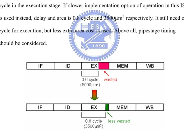
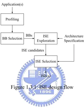
(11) Generally speaking, the number of ISEs can’t exceed number of unused opcode.. Total Silicon Area The total silicon area restricts extra area used by ASUF.. Pipestage Timing Because of the pipelining, the execution time of the ISE is the nearest integer cycle which is bigger than the delay of the ISE. Sometimes, there are several different implementation options for an operation, each has different delay and extra area cost. Figure 1.2.1 is an example. An ISE (delay = 0.6 cycle, area = 5000µm2) wastes 0.4 cycle in the execution stage. If slower implementation option of operation in this ISE is used instead, delay and area is 0.8 cycle and 3500µm2 respectively. It still need one cycle for execution, but less extra area cost is used. Above all, pipestage timing should be considered.. Figure 1.2.1: An example of pipestage timing. 1.3 ISE Design Flow The ISE design flow consists of application(s) profiling, basic block (BB) selection and ISE generation, shown in figure 1.3.1. After profiling, BB is selected as the input 10.

(12) of ISE exploration according to its execution time. ISE exploration finds frequently executed instruction patterns as ISE candidates which must conform to predefined constraints, such as input/output ports, ISA format, timing and instruction types. Under certain constraints, such as silicon area and ISA format, ISE selection selects ISEs which has the highest performance improvement among ISE candidates.. Application(s). Profiling. BB Selection. BBs. ISE Exploration. Architecture Specification. ISE candidates ISE Selection. ISE(s). Figure 1.3.1: ISE design flow. 1.4 Motivation Because of pipelining, if different implementation options of operations of ISE can be explored, then the wasted execution time may be decreased. Thus, extra area cost can be lower.. 1.5 Objective Considering pipestage timing in ISE exploration to reduce extra area cost of ISEs.. 11.

(13) Chapter 2 Relative Works and Background 2.1 Relative Works Instruction Set Extension (ISE) generation in the most works of [3, 4, 5, 6, 7, 9 and 13] consists of ISE exploration and ISE selection.. ISE exploration Authors in [3] propose an algorithm, called exact algorithm, to explore all possible ISE candidates such that it can be seen as an optimal solution. The exact algorithm maps the ISE search space, such as a basic block, to a binary tree and then discards some portion of the tree which violates predefined constraints. Nevertheless, this algorithm is highly computing-intensive so that it hardly processes a larger search space. For example, it must spend about one hour to process a search space consisting of only 30 instructions. To reduce the computing complexity, [3, 4] propose heuristic algorithms which are derived from the genetic algorithm and K-L algorithm respectively.. The work in [5] examines the impact of different constraints, such ISA format, hardware area and control flow, for ISE generation. These constraints would limit the performance improvement of the ISEs. ISA format limits the number of read and write ports to the register file. The limitation of control flow is whether the search space can cross basic block boundaries or not. In order to satisfy real-time constraints, 12.

(14) the search spaces are identified according to whether they locate on the worst-case execution path instead of execution time in [6]. This is because that the most frequently executed basic block or instruction may not contribute to the worst-case execution path. The granularity of each vertex within search space can be varied from one instruction to multiple subroutine calls in [13]. They also claim that one search space can consist of multiple basic blocks in their proposed algorithm.. From a different view point, [15] characterizes each basic block as a polynomial representation. At first, multiple-input single-output (MISO) algorithm extracts symbolic algebraic patterns from the search spaces and represents these patterns as polynomials on behalf of ISE candidates. Then these ISE candidates are mapped to the polynomial representations of program segments by symbolic algebraic manipulations.. ISE selection The work in [7] transforms ISE selection as an area minimization problem. There have been many relative researches of the area minimization problem in the logic synthesis domain. [8] proposes another algorithm that uses divide-and-conquer search technique to solve ISE selection. To synchronize pipeline between CPU core and ASFU, [9] first adjusts the timing of CPU core to same with ASFU if the execution time of ASFU is larger than CPU core. Then, different number of ASFU’s pipeline stage, from one, two, three … until no performance improvement, are evaluated. At meanwhile, timing of CPU core is also adjusted with ASFU. Finally, the number of ASFU’s pipestage with best performance improvement is then chosen.. In addition, to reduce hardware cost, [14] adds new stages, called ISE combination, 13.

(15) between ISE exploration and ISE selection stages, to merge multiple similar ISE candidates together.. 2.2 Background ─ Ant Colony Optimization (ACO). Algorithm Why Ant Colony Optimization Algorithm？ In order to indicate which part of a DFG is going to be ISE; the implementation of nodes should be decided. If we only consider the situation that there is only single hardware implementation option of a node, then there will be 2N possible ISE patterns (legal or illegal) that N is the DFG size. When N is 100 (it’s a usually case), the combinations is emphatic 2100！Obviously, this is a NP-hard problem. For the sake of an efficiently solution, the way of evolutionary computation which is operative to many existing NP-hard problems is considered.. There are many computation models belong to evolutionary computation, like genetic, simulated annealing, etc. One of them named “Ant Colony Optimization” is thought to be the easiest one to map to the problem. The selection among the models is processed by the difficulty of the mapping to the problem. An intuitive and easier mapping usually brings a simple and effective design of the algorithm.. One of the concepts of ACO is the selection a path among many choices (one or two or more) to get the shortest path. I think the selection among many different implementation options of each node is just like that. This is the main reason that ACO outperforms other models. The only problem is how do the nodes 14.

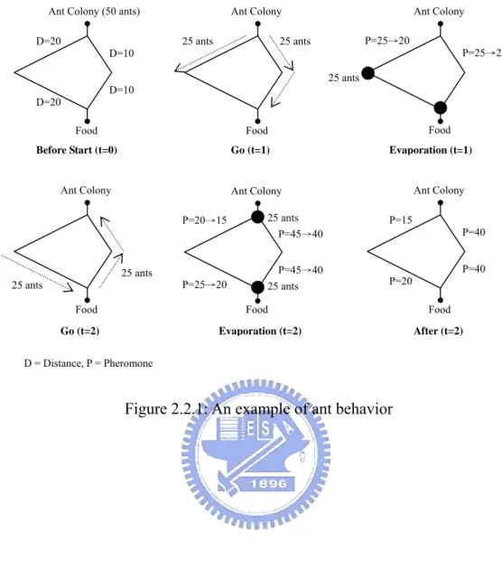
(16) “communicate” to each other. The merit computation in the design takes it into account.. Basic Idea of Ant Colony Optimization Algorithm Ant Colony Optimization algorithm is inspired by the behavior of ants in finding paths from the colony to food and has been extensively used to solve many optimization problems. Initially, ants wander randomly and lay down pheromone on the paths have been passed through. The density of the pheromone determines the probability of which path the next ant will pass through. Since the pheromone evaporates with the time, a shortest path gets marched over faster and thus has the higher density of pheromone. After a period of time, i.e. several iterations, more and more ants choose the shortest path such that the density of pheromone on this path grows increasingly. Finally, each ant almost chooses the shortest path and the pheromones of other paths evaporate to nearly zero.. Figure 2.2.1 is an example. Suppose 50 ants are in the ant colony. Now they are going to find food. There are two paths to get food. One is twice longer than the other. At t = 1, there is no pheromone on both paths. The ants choose paths with equal probability. Suppose 25 ants choose one path, and 25 ants choose another. One ant leaves one unit of pheromone on the path. But the pheromone evaporates 5 units after t = 1. So the paths ant passed has 25 – 5 = 20 pheromone. At t = 2, ants start again. After t = 2, we can see the pheromone on each path segment. Next time, the right hand side path will be chosen by ants with higher probability than the left hand side path.. 15.

(17) Ant Colony (50 ants) D=20. Ant Colony 25 ants. Ant Colony P=25→20. 25 ants. P=25→20. D=10 25 ants D=10 D=20 Food. Food. Food. Before Start (t=0). Go (t=1). Ant Colony. Evaporation (t=1). Ant Colony. Ant Colony 25 ants P=45→40. P=20→15. 25 ants 25 ants Food Go (t=2). P=45→40 25 ants. P=25→20. P=15 P=40 P=40 P=20. Food. Food. Evaporation (t=2). After (t=2). D = Distance, P = Pheromone. Figure 2.2.1: An example of ant behavior. 16.

(18) Chapter 3 ISE Exploration In this paper, the purpose of ISE exploration is to find frequently executed instruction patterns as ISE candidates and evaluates all implementation options of each operation in ISE candidates to minimize the execution time with less silicon area. The input and output of ISE exploration algorithm are BBs and ISE candidates as well as their implementation option, respectively. Implementation option(s) of an operation represents its implementation method(s), and can be roughly divided into two categories, hardware and software.. The flow of ISE exploration is briefly described as follows: each input BB is first transformed to data flow graphs (DFG), and an implementation option (IO) table which represents all implementation options for an operation is appended to each operation in DFG. In this extended DFG, ISE exploration algorithm is repeatedly executed until no ISE candidate can be found. Note that ISE exploration algorithm only explores one ISE candidate at each round. A round usually consists of multiple iterations. Initially, ISE exploration algorithm chooses one implementation option in each operation according to a probability value (p). The probability value (p) is a function of pheromone and merit values. The meaning of pheromone is the same with the pheromone in the ACO algorithm, i.e. how many times an implementation option is chosen in previous iterations. The merit value represents the benefit of one implementation option being chosen. After making a choice, the pheromone value is updated. And then, the algorithm evaluates implementation option of each operation 17.

(19) in DFG, i.e. calculates their merit value, according to which implementation option is chosen in its neighboring ones at previous iteration. Above process are iteratively performed until the probability values (p) of all operations in DFG have exceeded a predefined threshold value, P_END.. 3.1 Implementation option According to profiling results, a BB with longer execution time is transformed to DFG. A DFG is represented by a directed acyclic graph G(V,E) where V is a set of vertices and E is a set of directed edges. Each vertex v∈V represents an assembly instruction, called “operation” hereafter in BB. Each edge (u,v)∈E from operation u to operation v indicates that the execution of operation v requires the data produced by operation u.. Each operation usually has multiple implementation options which can be divided into two categories, hardware and software. Hardware implementation option means this operation is included in an ISE and implemented in extra hardware, i.e. ASFU. Due to different speed and area requirements, the operation usually has at least one hardware implementation option. On the other hand, software implementation option means this operation is executed in CPU core, and its execution time depends on the execution cycle count of each operation defined in CPU specification.. To represent all implementation options in a node, we add a table, called implementation option (IO) table, to each operation. Each entry in the IO table consists of one implementation option of the operation and its delay and area. Delay and area represent the execution cycle and the extra silicon area cost of this 18.

(20) implementation option, respectively. Obviously, using software implementation option for an operation requires one execution cycle at least but no extra silicon cost is introduced. On the other hand, using hardware implementation option can reduce execution cycle but consumes extra silicon area. After adding IO table to G, a new graph G+ is generated. Figure 3.1.1 shows an example of G+. This example consists of two operations, are A and B. In this example, we assume the delay of software implementation option as one cycle.. Figure 3.1.1: An example of G+. 3.2 Formulation of ISE Exploration ISE exploration explores ISE candidates in G+ and evaluates all implementation options of each operation in ISE candidates. An ISE candidate in G+ is a subgraph S ⊆G+. The proposed ISE exploration can be formulated as follows:. ISE exploration: Given a graph G+, find S⊆G+ and evaluate all implementation options of vertex v∈S to minimize the execution cycle count with less silicon area under the following constraints: 1. IN(S) ≤ Nin, 2. OUT(S) ≤ Nout,. 19.

(21) 3. S is convex, 4. Load and store operations ∉ S.. IN(S) (OUT(S)) represents the number of input (output) values used (produced) by Si. The user-defined values Nin and Nout indicate the register file read and write ports limitations, respectively. The convex constraint is that the ISE’s output can not connect to its input via other operations not grouped in ISE. In other words, if there exists no path from a operation u∈S to another operation v∈S which involves a operation w ∉ S, then S is convex. To conform to the limitation of RISC architecture and to degrade the complexity of the algorithm, load and store operations are prohibited from being grouped into ISE.. In fact, if the limitation of EX and MEM stage in usually pipeline can be eliminated, the execution and memory access can take place with non-certain sequence, then load and store operations are possibly grouped into ISE. And it is reasonably to enhance the benefit of ISE. 3.3 ISE Exploration Algorithm The ISE exploration algorithm is driven from ACO algorithm. Conceptually, we can imagine that one entry in IO table, i.e. one implementation option, represents one or part of path from colony to food in ACO algorithm. Exploring ISE candidate with evaluating different implementation options is just like an ant finding the shortest path from colony to food.. 20.

(22) Similar with ACO algorithm, which implementation option would be chosen depends on its probability value (p). The probability value (p) of each implementation option in an operation represents its probability of being chosen at each iteration of ISE exploration algorithm. On the other hand, choosing implementation option according to the probability value (p) can prevent local optimal solutions. The probability value (px,j) of j-th implementation option in operation x is a function of the pheromone and the merit values, as shown in equation (1). The meaning of the pheromone value is identical with the pheromone in the ACO algorithm. It reveals how many times an implementation option is chosen in previous iterations. Here, we denote the pheromone value of j-th implementation option of operation x by pheromonex,j in which pheromonex,0 is designated as the pheromone value of software implementation option. Just like the pheromone, the pheromone value must be updated after each iteration. The merit value is defined as the benefit of one implementation option being chosen, and it is calculated by the merit function which will be described in detail later. The merit value of j-th implementation option of operation x is denoted by meritx,j in which meritx,0 is designated as the merit value of software implementation option. The probability of j-th implementation option of operation x being chosen (px,j) is computed by:. px, j =. α ⋅ pheromonex , j + ( 1 − α) ⋅ merit x , j k. ∑ (α ⋅ pheromone j =0. x, j. , 0 ≤ j ≤ k and 0 ≤ α ≤ 1. (3.1). + ( 1 − α) ⋅ merit x , j ). where k is the number of hardware implementation options in operation x and α is used to determine the relative influence of pheromone and merit, and. 21.

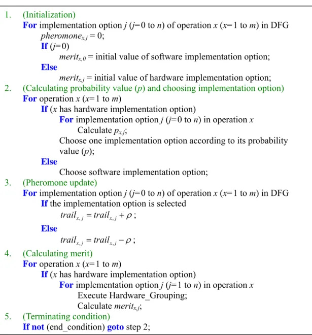
(23) k. ∑p j =0. x, j. =1. (3.2). Figure 3.3.1 shows the proposed ISE exploration algorithm. Here, we assume that there are m (m > 0) operations in a DFG and each operation has n (n > 0) implementation options. Initially, i.e. in step 1, the algorithm sets initial values for the pheromone and merit values of each implementation option of all operations. Note that the initial merit value of hardware and software implementation options is different. This is because we wish that the algorithm has higher has more opportunity to choose hardware implementation option at the beginning of execution. In step 2, the algorithm checks operation x (x=1 to m) whether it has hardware implementation option. If yes, the algorithm chooses one among all implementation options in operation x according to their probability values (px,j); if no, it chooses software implementation option.. In step 3, ISE exploration algorithm updates the pheromone value of each implementation option j in operation x (x=1 to m) according to whether the implementation option j is chosen or not. The pheromone value of chosen implementation option is increased with ρ, a positive constant value, and others are decreased with ρ. The algorithm in step 4 calculates the merit value of each implementation options in operation x. Same as in step 2, the algorithm also first checks operation x (x=1 to m) whether it has hardware implementation option. If yes, the algorithm executes Hardware Grouping function that determines whether operation x can be grouped with its neighboring ones as a virtual ISE candidate, if it can, Hardware-Grouping function uses this virtual ISE candidate to calculate the execution time and silicon area of each hardware implementation option in operation. 22.

(24) x. We will describe Hardware-Grouping function in detail later. And then, the merit value (meritx,j) of implementation option j (j=1 to n) in operation x is generated by using merit function. Finally, ISE exploration algorithm checks the end condition in step 5. If the end condition is not satisfied, ISE exploration algorithm returns to step 2 and enters the next iteration; else, it terminates.. 1.. 2.. 3.. (Initialization) For implementation option j (j=0 to n) of operation x (x=1 to m) in DFG pheromonex,j = 0; If (j=0) meritx,0 = initial value of software implementation option; Else meritx,j = initial value of hardware implementation option; (Calculating probability value (p) and choosing implementation option) For operation x (x=1 to m) If (x has hardware implementation option) For implementation option j (j=0 to n) in operation x Calculate px,j; Choose one implementation option according to its probability value (p); Else Choose software implementation option; (Pheromone update) For implementation option j (j=0 to n) of operation x (x=1 to m) in DFG If the implementation option is selected trail x , j = trail x , j + ρ ; Else. 4.. 5.. trail x , j = trail x , j − ρ ; (Calculating merit) For operation x (x=1 to m) If (x has hardware implementation option) For implementation option j (j=1 to n) in operation x Execute Hardware_Grouping; Calculate meritx,j; (Terminating condition) If not (end_condition) goto step 2; Figure 3.3.1: ISE Exploration Algorithm. The end condition is that for all operations in DFG, the probability value (p) of one of implementation options exceeds P_END which is a predefined threshold value and 23.

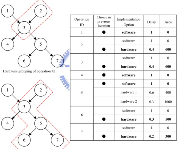
(25) very closed to 100%. A larger P_END have greater opportunity to obtain better result, but it needs longer convergence time, i.e. takes more computing time. An implementation option with the probability value (p) over P_END is called taken implementation option. A single ISE candidate is a group of connected operations in the DFG which all have taken hardware implementation option.. Hardware-Grouping If the operation x has hardware implementation option, a function, called Hardware-Grouping, must be executed before computing the merit value of each hardware implementation option. Hardware-Grouping checks whether the operation x can be grouped with its neighboring ones as a virtual ISE candidate. It recursively groups operation x with neighboring ones which have chosen hardware implementation option in previous iteration as a virtual ISE candidate, i.e. a virtual subgraph vSx. Here, we denote the result of Hardware-Grouping of operation x using. j-th implementation option by vSx,j. Note that vSx,0 is meaningless due to 0-th implementation option is software one. Using the vSx,j, Hardware-Grouping evaluates the execution time and silicon area of vSx,j. Note that the execution time of vSx,j is the critical path time in vSx,j and the silicon area of vSx,j is the sum of silicon area of vSx,j.. We use figure 3.3.2 to explain how the Hardware-Grouping operates. The table in figure 3.3.2 represents delay and area of each implementation option for all operations and specifies the chosen implementation option in previous iteration. In both top and bottom left of figure 3.3.2, nodes in dotted line are treated as a virtual ISE candidate. For operation #2, Hardware-Grouping groups operation #2 and #3 as a virtual ISE candidate, i.e. vS2, as shown in the top left of figure 3.3.2. Since only one hardware implementation option exists in operation #2, vS2 has one evaluating result in. 24.

(26) execution time and silicon area (execution time = 0.8, silicon area = 1200). The bottom left of figure 3.3.2 is another example in which Hardware-Grouping groups operation #5 and its neighboring ones, are #2, #3, #6 and #7, as a virtual ISE candidate, i.e. vS5. Since operation #5 has two hardware implementation options, there are two evaluating results in vS5, one is vS5,1 (execution time = 1.7, silicon area = 2400) and another is vS5,2 (execution time = 1.4, silicon area = 3000).. 1. 2 ID. Choice in previous iteration. 1. ●. Operation. 3 4. 5. Delay. Area. software. 1. 0. software. 1. 0. hardware. 0.4. 600. software. 1. 0. ●. hardware. 0.4. 600. ●. software. 1. 0. ●. software. 1. 0. 7. Hardware grouping of operation #2. 1. hardware 1. 0.6. 400. hardware 2. 0.3. 1000. software. 1. 0. hardware. 0.3. 500. software. 1. 0. hardware. 0.2. 300. Option. 2 ●. 6. Implementation. 3 4. 2. 5. 3 6. 4. ●. 5 7. 6. ●. 7. Hardware grouping of operation #5. Figure 3.3.2: Examples of Hardware-Grouping Merit Function The purpose of merit function is to calculate the benefit, i.e. merit value, of implementation option. Briefly, the merit function consists of three cases: size checking (case 1), constraints violation determination (case 2) and benefit calculating 25.

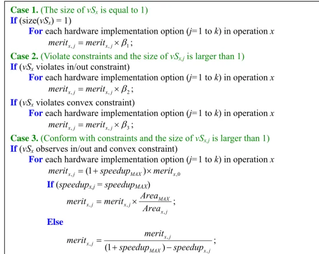
(27) (case 3). Figure 3.3.3 depicts the algorithm of merit function. Initially, in the case 1, the algorithm checks whether size(vSx,j), is denoted as the number of operation in vSx,j, is equal to one. If yes, since there is only one operation, i.e. operation x, in vSx,j, it is impossible to improve performance, so that the algorithm adjusts the merit value to decrease the chance of choosing hardware implementation option, this comparatively rises the choosing probability of software implementation option. And then, the calculation of merit function is terminated. Note that in this paper, we assume each operation is one-cycle delay. If multiple-cycle delay is assumed, case 1 may be tailored to fit the situation. If no, goto case 2.. The case 2 checks whether vSx violates input/output port and convex constraints. If yes, the merit value of each hardware implementation option is multiplied by a constant β1, β2 or β3 (0 < β1 < 1, 0 < β2 < 1 and 0 < β3 < 1). This relatively reduces the opportunity of selection of software implementation option just the same as in case 1. And then, the calculation of merit function is terminated. The reason why we only divide the merit value of each hardware implementation option in operation x by a constant rather than exclude the possibility of operation x becoming an ISE candidate is that operation x will have an opportunity to be grouped as an ISE candidate in the next iteration. If no, enter case 3.. In the case 3, the merit value of j-th implementation option (meritx,j, j > 0) in the operation x is calculated according to (1) how much speed up can be achieved by vSx,j; or (2) the extra area used by vSx,j. The execution time, cycle reduction and silicon area of the virtual subgraph vSx,j is denoted by ET(vSx,j), speedupx,j and areax,j, respectively. The basic idea is (1) if vSx,j can improvement the performance, j-th implementation option should have larger merit value than software implementation; (2) if a hardware 26.

(28) implementation option in the operation x has higher cycle reduction, it should have larger merit value than lower ones; and (3) if several hardware implementation options in the operation x have the highest cycle reduction, the one uses less extra silicon area should have higher merit value. Based on above, the merit value of j-th implementation option is first multiplied by speedupMAX which the maximal speedup can be achieved in operation x. Than, if the speedup of j-th implementation option is equal to speedupMAX, the merit value of j-th implementation option is scaled by the silicon area used for j-th implementation option. AreaMAX is the largest silicon area used in operation x. Otherwise, the merit of j-th implementation option is scaled by the speedup of this hardware implementation option.. Case 1. (The size of vSx is equal to 1) If (size(vSx) = 1) For each hardware implementation option (j=1 to k) in operation x merit x , j = merit x , j × β1 ; Case 2. (Violate constraints and the size of vSx,j is larger than 1) If (vSx violates in/out constraint) For each hardware implementation option (j=1 to k) in operation x merit x , j = merit x , j × β 2 ; If (vSx violates convex constraint) For each hardware implementation option (j=1 to k) in operation x merit x , j = merit x , j × β3 ; Case 3. (Conform with constraints and the size of vSx,j is larger than 1) If (vSx observes in/out and convex constraint) For each hardware implementation option (j=1 to k) in operation x merit x , j = (1 + speedupMAX ) × merit x ,0 If (speedupx,j = speedupMAX) AreaMAX ; merit x , j = merit x , j × Areax , j Else merit x , j merit x , j = ; (1 + speedupMAX ) − speedupx , j Figure 3.3.3: Algorithm of merit function. 27.

(29) 3.4 Optimal Solution The optimal solution can be identified as follows. At first, step 1, all of the possible patterns in the DFG are enumerated and tested to the input/output and convex constraints, and those passed the test are listed as legal ISEs. In step 2, exact implementation option evaluation of each ISE in the list is calculated. Suppose the DFG size is n and there are k legal ISEs are listed and the maximum hardware implementation option number is c, then the time complexity of step 1 and step 2 are O(2n)·O(n) and k·O(cn)·O(n) respectively. Finally in step 3, all of the combinations of legal ISEs are enumerated, and then we can get the best cycle reduction number and corresponding minimum area cost of the DFG. The complexity of this step is O(2k).. 28.

(30) Chapter 4 ISE Selection Due to the constraints of silicon area and original ISA format, the subset of ISE candidates which has the best performance improvement under the constraints should be selected. This problem is formulated as the multi-constrained 0/1 Knapsack problem as follows:. ISE selection: Suppose there are n ISE candidates, the area of the ith ISE is ai and the. performance improvement of the ith ISE is wi, the area of selected ISEs can’t exceed the total area A, the limitation of the number of extended instructions is E, and then get the maximum of. n. f ( x1 ,..., xn ) = ∑ wi xi and xi ∈ {0,1} ， 1 ≤ i ≤ n. (4.1). i =1. where xi is 1 if the ith ISE is selected, and vice versa, and subject to. n. n. i =1. i =1. ∑ xi ≤ E ， ∑ ai xi ≤ A and xi ∈ {0,1} ，1 ≤ i ≤ n. (4.2). Noticeable, the constraints on ISE selection in this paper are silicon area and original ISA format. However, if we add new constraints on ISE selection, only the equation (4.2) needs to be changed as follows:. 29.

(31) n. C j : ∑ cti , j xi ≤ b j and xi ∈ {0,1} ， 1 ≤ i ≤ n. (4.3). i =1. where Cj represents which constraint is applied, cti,j is resource consumption values of ith ISE and bj is the given resource limits.. 30.

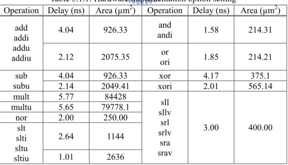
(32) Chapter 5 Experimental Results 5.1 Experimental setup We use Portable Instruction Set Architecture (PISA) [10] which is a MIPS-like ISA and MiBench [11] with different register input/output ports constraint to evaluate our proposed algorithm. Each benchmark is compiled by gcc 2.7.2.3 for PISA with -O0 and -O3 optimizations. Due to the limitation in library and compiler, 6 benchmarks, such as mad, typeset, ghostscript, rsynth, sphinx and pgp, can not be compiled successfully. For both algorithms, we evaluate 6 cases, includes 2/1, 4/2 and 6/3 register file read/write ports as well as using -O0 and -O3 optimization. Table 5.1.1: Hardware implementation option setting Operation Delay (ns) Area (µm2) Operation Delay (ns) Area (µm2) add addi addu addiu. 4.04. 926.33. and andi. 1.58. 214.31. 2.12. 2075.35. or ori. 1.85. 214.21. sub subu mult multu nor slt slti sltu sltiu. 4.04 2.14 5.77 5.65 2.00. 926.33 2049.41 84428 79778.1 250.00. xor xori. 4.17 2.01. 375.1 565.14. 2.64. 1144. 3.00. 400.00. 1.01. 2636. sll sllv srl srlv sra srav. In this simulation, we assume that: (1) the CPU core is synthesized in 0.13 µm CMOS technology and executes in 100MHz; (2) the CPU core area is 1.5 mm2; (3) the 31.

(33) read/write ports of register file are 2/1, 4/2 and 6/3, respectively; and (4) the execution time of all instructions in PISA is one cycle, i.e. 10 (ns). Table 5.1.1 shows the hardware implementation option settings (delay and area) of instructions in PISA. Note that we only list instructions which are capable of being grouped into ISE in table 5.1.1. These settings reference from either [12] or synthesized by Synopsys Design Compiler with standard cells. Since increasing the read/write ports of register file needs extra silicon area, we also synthesize different read/write ports of register file. The silicon area of CPU core with 4/2 and 6/3 (register file read/write ports) are 1574138.80µm2 and 1631359.54µm2, respectively.. Because of the heuristic nature of the ISE exploration algorithm, the exploration is repeated 5 times within each basic block, and the result among the 5 iterations having minimal execution cycle count with less extra area cost is selected.. To make things easy as much as possible, the parameters are usually fixed and to adjust one of them one at a time. For the sake of clarity, one parameter is designed to influence only one thing, although they usually effect with each other. For example, the parameter β decides the decay speed of merit when one of the constraints is violated. When we have a fitting magnitude of β, there are always other things changed at the same time due to the alternation of β. Then we adjust other parameters one at a time just like we did to β. After many times of regulation, we can find that the interval of the parameter at each regulation is less and less. Finally, we get a set of suitable parameters.. The following is the parameters in this paper and their meaning. α：The weight of merit and pheromone in px,j. Increase α to get a solution more slowly, 32.

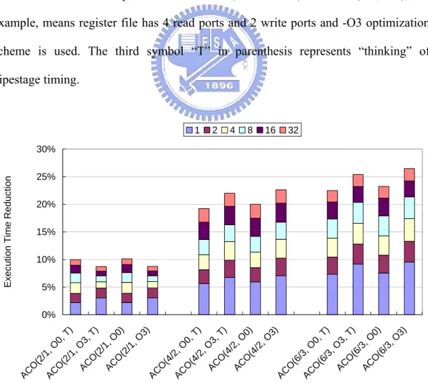
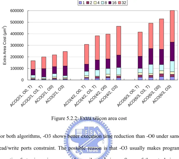
(34) decrease α to get a solution more quickly, but usually worse one. β1：The tendency to choose hardware implementation option in a node. β2：The decay speed when the input/output constraint is violated. β3：The decay speed when the convex constraint is violated.. In our experiments, we use the initial value of software implementation option of 100, initial value of hardware implementation option of 200, P_END of 99%. The parameter α used in the calculation of probability value, β1, β2 and β3 used in merit function are 0.25, 0.9, 0.9 and 0.5, respectively.. In the simulation, the ISE selection is implemented as a greedy algorithm. ISE number and silicon area constraints can be easily applied within the greedy algorithm. ISE selection algorithm first sorts ISE candidates according to their cycle count reduction. The ISEs are then selected sequentially according to this sorted list until the number of ISEs exceeds ISE number constraint or total silicon area is over. For the sake of clarity, the simulation result only shows the impact of the ISE number constraint. We divide the total saving cycle count of selected ISEs by the total cycle count of original application to get the execution time reduction in the figures.. 5.2 Experimental results Figure 5.2.1 and 5.2.2 show the average execution time reduction and average extra silicon area cost of Mibench, respectively, under different number of ISE. In both figure 5.2.1 and 5.2.2, each bar consists of several segments which indicate the execution time reduction under different number of ISE, are 1, 2, 4, 8, 16 and 32, respectively. 33.

(35) In order to show the effectiveness of the consideration of pipestage timing is remarkable. We assume the proposed algorithm doesn’t consider the effect of pipestage timing. Therefore there is only one hardware implementation option for the operation can be included into ISE. In here, we always take it as the fastest implementation option.. The label on X axis in both figure 5.2.1 and 5.2.2 represents ISE exploration algorithm with different arguments is used. The first and second symbols in parenthesis of each label on X axis represent the number of register file read/write ports used and which optimization scheme (-O0 or -O3) is used. (4/2, O3), for example, means register file has 4 read ports and 2 write ports and -O3 optimization scheme is used. The third symbol “T” in parenthesis represents “thinking” of pipestage timing.. 1. 2. 4. 8. 16. 32. 25% 20% 15% 10% 5% 0%. AC O (2 / AC 1, O O 0, (2 T) /1 ,O AC 3, T) O (2 /1 AC ,O O 0) (2 /1 ,O 3) AC O (4 / AC 2, O O 0, (4 T) /2 ,O AC 3, T) O (4 /2 AC ,O O 0) (4 /2 ,O 3) AC O (6 / AC 3, O O 0, (6 T) /3 , AC O3 ,T O ) (6 /3 AC ,O O 0) (6 /3 ,O 3). Execution Time Reduction. 30%. Figure 5.2.1: Execution time reduction 34.

(36) 1. 2. 4. 8. 16. 32. 600000. 2. Extra Area Cost (µm ). 500000 400000 300000 200000 100000. AC O (2 / AC 1, O O 0, (2 T) /1 ,O AC 3, T) O (2 /1 AC ,O O 0) (2 /1 ,O 3) AC O (4 / AC 2, O O 0, (4 T) /2 ,O AC 3, T) O (4 / AC 2, O O 0) (4 /2 ,O 3) AC O (6 / AC 3, O O 0, (6 T) /3 ,O AC 3, T) O (6 /3 AC ,O O 0) (6 /3 ,O 3). 0. Figure 5.2.2: Extra silicon area cost For both algorithms, -O3 shows better execution time reduction than -O0 under same read/write ports constraint. The possible reason is that -O3 usually makes program execution faster in various ways of compiler techniques. Some of these techniques (like loop unrolling, function inlining, etc.) remove branch instructions and increase the size of certain critical basic blocks. The bigger the basic block size is, the larger the search space exists and the more possibility the ISEs which have more cycle reduction can be explored in these bigger basic blocks. Also noteworthy is that most of execution time reduction is contributed by several ISEs. This is because the execute time of most program takes on small fraction of code segment, i.e. the execution time reduction is dominated by several ISEs. In most cases, 8 ISEs can achieve half or more of execution time reduction and only consume a little fraction of the maximum extra area cost. For example, 8 ISEs using 4/2 (register file read/write ports) register file can save average 14.95% execution time and cost 81467.5µm2 silicon area, that’s 5.43% of the original core area. On the other hand, if we select 32 ISEs, the average 35.

(37) execution time reduction can increase to 20.62% but extra area cost also rises to 345135.45µm2, that’s 23.01% of the original core area.. There is one thing should be noticed in figure 5.2.1 that ACO (2/1, O0) seems to be better than ACO (2/1, O3). In fact, with 1, 2 and 4 ISE number, –O3 still behaves better than –O0, the situation reverses only with larger ISE number. This is caused by the results of some special benchmark. For example, there are only 4 ISEs can be found by –O3, but –O0 can find over 4 ISEs and totally get more execution time reduction. When the ISE number is more than 4, then –O0 looks like better than –O3.. ACO(2/1, O0, T). ACO(2/1, O3, T). ACO(4/2, O0, T). ACO(4/2, O3, T). ACO(6/3, O0, T). ACO(6/3, O3, T). 35%. Extra Area Saving Percentage. 30% 25% 20% 15% 10% 5% 0% 1. 2. 4. 8. 16. 32. ISE Number. Figure 5.2.3: Extra area saving percentage Since the proposed ISE exploration algorithm explores not only ISE candidate but also their implementation option, less extra silicon area is used in all cases. Figure 5.2.3 illustrates the extra area saving percentage for all cases and figure 5.2.4 to figure 5.2.6 shows the execution time reduction per unit area. In these figures, the. 36.

(38) consideration of pipestage timing obviously reduces the extra area usage.. ACO(2/1, O0, T). ACO(2/1, O3, T). ACO(2/1, O0). ACO(2/1, O3). Execution Time Reduction per Unit Area. 10.00 9.00 8.00 7.00 6.00 5.00 4.00 3.00 2.00 1.00 0.00 1. 2. 4. 8. 16. 32. ISE Number. Figure 5.2.4: Execution time reduction per unit area (2/1). ACO(4/2, O0, T). ACO(4/2, O3, T). ACO(4/2, O0). ACO(4/2, O3). Execution Time Reduction per Unit Area. 10.00 9.00 8.00 7.00 6.00 5.00 4.00 3.00 2.00 1.00 0.00 1. 2. 4. 8. 16. ISE Number. Figure 5.2.5: Execution time reduction per unit area (4/2). 37. 32.

(39) ACO(6/3, O0, T). ACO(6/3, O3, T). ACO(6/3, O0). ACO(6/3, O3). Execution Time Reduction per Unit Area. 10.00 9.00 8.00 7.00 6.00 5.00 4.00 3.00 2.00 1.00 0.00 1. 2. 4. 8. 16. 32. ISE Number. Figure 5.2.6: Execution time reduction per unit area (6/3) From another perspective, under the same silicon area constraints, using miser implementation option can employ more ISEs in processor core. This leads to better performance improvement. We illustrate this perspective with figure 5.2.7 and 5.2.8. In figure 5.2.7, each bar consists of several segments which indicate the execution time reduction under different silicon area constraint, are 5%, 10%, 15%, 20%, 25% and 30% of original CPU core, respectively. Figure 5.2.8 shows ISE number can be used in different silicon area constraint. Note that the silicon area of CPU core with different register file read/write ports is different. In all cases, the proposed ISE exploration algorithm has better improvement in the execution time reduction. It is more noteworthy that the improvement of execution time reduction is not in proportion to available silicon area. This is because most execution time reduction is dominated by several ISEs. Table 5.2.1 shows the detailed results of figure 5.2.7 and 5.2.8.. 38.

(40) 5%. 10%. 15%. 20%. 25%. 30%. Execution Time Reduction. 30% 25% 20% 15% 10% 5%. AC O (2 / AC 1, O O 0, (2 T) /1 ,O AC 3, T) O (2 /1 AC ,O O 0) (2 /1 ,O 3) AC O (4 / AC 2, O O 0, (4 T) /2 ,O AC 3, T) O (4 /2 AC ,O O 0) (4 /2 ,O 3) AC O (6 / AC 3, O O 0, (6 T) /3 ,O AC 3, T) O (6 /3 AC ,O O 0) (6 /3 ,O 3). 0%. Figure 5.2.7: Execution time reduction under different silicon area constraint. 5%. 10%. 15%. 20%. 25%. 30%. 100 90 80 ISE Number. 70 60 50 40 30 20 10. AC O (2 / AC 1, O O 0, (2 T) /1 ,O AC 3, T) O (2 /1 AC ,O O 0) (2 /1 ,O 3) AC O (4 / AC 2, O O 0, (4 T) /2 ,O AC 3, T) O (4 /2 AC ,O O 0) (4 /2 ,O 3) AC O (6 / AC 3, O O 0, (6 T) /3 ,O AC 3, T) O (6 /3 AC ,O O 0) (6 /3 ,O 3). 0. Figure 5.2.8: ISE Number under different silicon area constraint Table 5.2.1: Execution time reduction under different silicon area constraint Silicon area 5% 10% 15% 20% 25% constraint Number of ISE being selected ACO(2/1, O0, T) 13 28 50 71 102 39. 30% 128.

(41) ACO(2/1, O3, T). 12. 27. 40. 55. 79. 100. ACO(2/1, O0). 10. 21. 34. 50. 64. 86. ACO(2/1, O3). 10. 72. ACO(2/1, O0, T). 8.60%. 19 31 44 55 Execution time reduction 9.81% 10.38% 10.61% 10.76%. ACO(2/1, O3, T). 7.57%. 8.49%. 8.94%. 9.29%. 9.54%. 9.64%. ACO(2/1, O0). 6.49%. 7.21%. 7.61%. 7.90%. 8.02%. 8.11%. ACO(2/1, O3). 6.65%. 7.28% 7.72% 8.01% 8.20% Number of ISE being selected 18 23 34 46. 8.36%. 10.83%. ACO(4/2, O0, T). 8. 56. ACO(4/2, O3, T). 6. 14. 20. 26. 34. 45. ACO(4/2, O0). 6. 13. 20. 24. 32. 42. ACO(4/2, O3). 5. 33 20.64%. ACO(4/2, O0, T). 13.61%. 12 17 22 27 Execution time reduction 17.26% 18.19% 19.31% 20.13%. ACO(4/2, O3, T). 14.98%. 19.04%. 20.46%. 21.30%. 22.09%. 22.84%. ACO(4/2, O0). 12.13%. 15.06%. 16.69%. 17.27%. 18.08%. 18.77%. ACO(4/2, O3). 14.15%. 17.51% 18.64% 19.43% 20.04% Number of ISE being selected 12 19 25 31. 20.62%. ACO(6/3, O0, T). 5. 39. ACO(6/3, O3, T). 6. 9. 14. 19. 25. 32. ACO(6/3, O0). 4. 9. 15. 19. 24. 29. ACO(6/3, O3). 4. 25 22.87%. ACO(6/3, O0, T). 14.95%. 7 11 15 20 Execution time reduction 19.25% 20.97% 21.77% 22.33%. ACO(6/3, O3, T). 18.76%. 20.92%. 22.72%. 23.77%. 24.61%. 25.32%. ACO(6/3, O0). 13.83%. 17.19%. 19.37%. 20.19%. 20.94%. 21.56%. ACO(6/3, O3). 16.91%. 19.76%. 21.74%. 22.92%. 24.00%. 24.81%. 5.3 Optimal Solution In order to illustrate the quality of ISEs explored by the proposed algorithm, a set of basic blocks are processed to get the optimal solution. In table 5.3.1, we compare the result of proposed algorithm and the optimal solution. And the corresponding processing time is listed in table 5.3.2. The legal pattern number is the number of 40.

(42) patterns that are legal to be ISEs (input/output constraint, convex, no load/store operation). The processing time of the optimal solution of a DFG is decided by the DFG size or legal pattern number. This can be observed from the time complexity of optimal solution mentioned earlier. For the cases that optimal solution can be obtained successfully, the proposed algorithm exhibits wonderful solution quality compared to the optimal one. It can get cycle reduction and extra area cost closed to the optimal one with tremendous computing time saving. For the legal pattern number up to 45 or even 108, the optimal solution needs considerable computing time and even can’t terminate in a reasonable interval. On the other hand, the proposed algorithm just consumes a few seconds to get the solution. Another observation is the released input/output constraint usually leads the increment of legal pattern number. In this situation, to obtain the optimal solution is more difficult, but proposed algorithm still behaves well. Table 5.3.1: Comparison of optimal solution and ISE Exploration Algorithm (result) DFG Size 13. Legal Optimal Solution In / Out Pattern Cycle Extra Area Constraint Number Reduction Cost 4 2/1 3 1228. Proposed Algorithm Cycle Extra Area Reduction Cost 3 1228. 26. 9. 2/1. 5. 7381. 5. 7603. 20. 30. 2/1. 8. 11683. 6. 9152. 41. 7. 2/1. 7. 10028. 7. 10028. 64. 1. 2/1. 1. 1141. 1. 1141. 32. 45. 2/1. --*. --. 16. 107160. 23. 75. 2/1. --. --. 9. 13886. 13. 2/1. 5. 6454. 4. 5128. 28. 4/2. 6. 8752. 6. 8752. 13. 2/1. 9. 9127. 9. 9350. 46. 4/2. --. --. 13. 13929. 108. 6/3. --. --. 15. 14357. 12. 44. P.S. *: means the solution can’t be obtained in practical time.. 41.

(43) Table 5.3.2: Comparison of optimal solution and ISE Exploration Algorithm (processing time) DFG Size 13. Legal Optimal Solution Proposed Algorithm In / Out Pattern Processing Processing Constraint Number Time Time 4 2/1 0.01s 0.03s. 26. 9. 2/1. 0.03s. 1.21s. 20. 30. 2/1. 14m22.46s. 2.705s. 41. 7. 2/1. 2m12.53s. 1.249s. 64. 1. 2/1. 4.08s. 0.753s. 32. 45. 2/1. --*. 4.49s. 23. 75. 2/1. --. 2.333s. 13. 2/1. 0.01s. 0.438s. 28. 4/2. 2m15.33s. 0.777s. 13. 2/1. 4.73s. 1.786s. 46. 4/2. --. 2.102s. 108. 6/3. --. 3.067s. 12. 44. P.S. *: means the solution can’t be obtained in practical time.. 42.

(44) Chapter 6 Conclusion The proposed ISE exploration and selection algorithms can significantly reduce extra silicon area cost with almost no performance loss. Previous researches, to achieve the highest speed-up ratio, overlook several important microarchitectural constraints, such as pipestage timing constraint and instruction set architecture (ISA) format. To conform to pipestage timing constraint, an ISE exploration algorithm which evaluates different implementation options of each operation in DFG during exploring ISE candidates is proposed. On the other hand, we formulate ISE selection as the multi-constrained 0/1 Knapsack problem to comply with different microarchitectural constraints. The benefits of our approach are: (1) conform to several important microarchitectural constraints; (2) significantly reduce extra silicon area cost; (3) both algorithms are polynomial time solvable. Experiment results show that our design can further reduce up to 35.28%, 15.92% and 22.41% (max., min. and avg.) of extra silicon area, and only has maximally 1.06% performance loss.. In addition, we conclude several issues which can be addressed in future work. First, with adjusting parameters (α, β1, β2 and β3) used in probability value, ISE exploration algorithm and merit function, we observe that these parameters greatly affect experimental results. Although we only use a same set of parameters for different cases, i.e. different combination of register file read/write ports and the size of BB, in this work, it will be an interesting if we study the dynamic adjustment for these parameters in our approach. Second, the running time of ISE generation algorithm is 43.

(45) one noteworthy issue. In this paper, ISE exploration algorithm only explores one ISE candidate at each round. However, if the algorithm simultaneously explores multiple ISE candidates at each round, the running time can significantly be reduced. Third, [combination] raises one interesting issue “ISE combination”. Without introducing any performance loss, if we merge several analogous ISE candidates as one or use one hardware resource to execute identical operations in same ISE, the silicon area can be further reduced.. 44.

(46) Reference [1] Gang Wang, Wenrui Gong and Ryan Kastner, “Application Partitioning on Programmable Platforms Using the Ant Colony Optimization”, to appear in the Journal of Embedded Computing, Vol. 2, Issue 1, 2006. [2] Mouloud Koudil, Karima Benatchba, Said Gharout, Nacer Hamani: Solving Partitioning Problem in Codesign with Ant Colonies. IWINAC (2) 2005: 324-337. [3] Laura Pozzi, Kubilay Atasu, and Paolo Ienne. Exact and Approximate Algorithms for the Extension of Embedded Processor Instruction Sets. Computer-Aided Design of Integrated Circuits and Systems, IEEE Transactions on Volume 25, Issue 7, Jul 2006 Page(s):1209 – 1229. [4] Partha Biswas, Sudarshan Banerjee, Nikil Dutt, Laura Pozzi, and Paolo Ienne. Fast automated generation of high-quality instruction set extensions for processor customization. In Proceedings of the 3rd Workshop on Application Specific Processors, Stockholm, September 2004. [5] Pan Yu, Tulika Mitra: Characterizing embedded applications for instruction-set extensible processors. DAC 2004: 723-728. [6] Pan Yu, Tulika Mitra: Satisfying real-time constraints with custom instructions. CODES+ISSS 2005: 166-171. [7] Jason Cong, Yiping Fan, Guoling Han, Zhiru Zhang. Application-Specific Instruction Generation for Configurable Processor Architectures. Twelfth International Symposium on Field Programmable Gate Arrays, 183-189, 2004. [8] Samik Das, P. P. Chakrabarti, Pallab Dasgupta: Instruction-Set-Extension Exploration Using Decomposable Heuristic Search. VLSI Design 2006: 293-298. [9] F. Sun, S. Ravi, A. Raghunathan, and N. K. Jha, "Custom-Instruction Synthesis for Extensible-Processor Platforms," IEEE Transactions on Computer-Aided Design of Integrated Circuits and Systems, vol. 23, pp. 216--228, February 2004. [10] T. Austin, E. Larson, and D. Ernst. SimpleScalar: An infrastructure for computer system modeling. IEEE Computer, 35(2), 2002. [11] M. R. Guthaus et al. Mibench: A free, commercially representative embedded benchmark suite. In IEEE Annual Workshop on Workload Characterization, 2001. [12] A Lindstrom and M. Nordseth. (2004, Mars). Arithmetic Database. [Online]. Available: http://www.ce.chalmers.se/arithdb/ [13] Edson Borin, Felipe Klein, Nahri Moreano, Rodolfo Azevedo, and Guido Araujo. “Fast Instruction Set Customization”, 2nd Workshop on Embedded Systems for 45.

(47) Real-Time Multimedia (ESTIMedia'04). Stockholm - Sweden, September 2004. [14] Nathan T. Clark, Hongtao Zhong, Scott A. Mahlke, "Automated Custom Instruction Generation for Domain-Specific Processor Acceleration," IEEE Transactions on Computers, vol. 54, no. 10, pp. 1258-1270, Oct., 2005. [15] Armita Peymandoust, Laura Pozzi, Paolo Ienne, and Giovanni De Micheli. Automatic Instruction-Set Extension and Utilization for Embedded Processors. In Proceedings of the 14th International Conference on Application-specific Systems, Architectures and Processors, The Hague, The Netherlands, June 2003. [16] A. Lindström, M. Nordseth and L. Bengtsson. "0.13 µm CMOS Synthesis of Common Arithmetic Units", Technical Report 03-11, Department of Computer Engineering, Chalmers University of Technology, June 2003. [17] Laura Pozzi, Paolo Ienne: Exploiting pipelining to relax register-file port constraints of instruction-set extensions. CASES 2005: 2-10. [18] Maria Luisa Lopez-Vallejo, Jesus Grajal, Juan Carlos Lopez, "Constraint-Driven System Partitioning," date, p. 411, Design, Automation and Test in Europe (DATE '00), 2000.. 46.

(48) 47. 70.00%. 60.00%. 50.00%. 40.00%. 30.00%. 20.00%. 10.00%. 0.00% CRC32_O0. sha_O3. sha_O0. rijndael_O3. rijndael_O0. blowfish_O3. blowfish_O0. stringsearch_O3. FFT_O3 adpcm_O0 adpcm_O3 gsm_O0 gsm_O3 average. FFT_O3. adpcm_O0. adpcm_O3. gsm_O0. gsm_O3. average. FFT_O0. 32 CRC32_O3. Execution time reduction of ACO(4/2, T). FFT_O0. Figure A.1.1: Execution time reduction of ACO(2/1, T). CRC32_O3. CRC32_O0. sha_O3. sha_O0. rijndael_O3. rijndael_O0. blowfish_O3. blowfish_O0. stringsearch_O3. 16 stringsearch_O0. ispell_O3. ispell_O0. patricia_O3. 16. stringsearch_O0. ispell_O3. 8. ispell_O0. dijkstra_O3 patricia_O0. 8. patricia_O3. 4. patricia_O0. dijkstra_O0. tiffmedian_O3. 4. dijkstra_O3. 2. dijkstra_O0. tiffdither_O3 tiffmedian_O0. 2. tiffmedian_O3. 1. tiffmedian_O0. tiffdither_O0. tiff2rgba_O3. tiff2rgba_O0. tiff2bw_O3. tiff2bw_O0. lame_O3. lame_O0. djpeg_O3. djpeg_O0. cjpeg_O3. cjpeg_O0. susan_O3. susan_O0. qsort_O3. qsort_O0. bitcount_O3. bitcount_O0. basicmath_O3. basicmath_O0. 1. tiffdither_O3. tiffdither_O0. tiff2rgba_O3. tiff2rgba_O0. tiff2bw_O3. tiff2bw_O0. lame_O3. lame_O0. djpeg_O3. djpeg_O0. cjpeg_O3. cjpeg_O0. susan_O3. susan_O0. qsort_O3. qsort_O0. bitcount_O3. bitcount_O0. basicmath_O3. Execution time reduction. A.1.. basicmath_O0. Execution time reduction. Appendix A. Simulation results of ACO(Input/Output, T) Execution time reduction of ACO(2/1, T) 32. 70.00%. 60.00%. 50.00%. 40.00%. 30.00%. 20.00%. 10.00%. 0.00%.

(49) 48. 70.00%. 60.00%. 50.00%. 40.00%. 30.00%. 20.00%. 10.00%. 0.00%. Figure A.1.4: Execution time reduction of ACO(8/4, T) CRC32_O0. sha_O3. sha_O0. rijndael_O3. rijndael_O0. blowfish_O3. blowfish_O0. stringsearch_O3. FFT_O3 adpcm_O0 adpcm_O3 gsm_O0 gsm_O3 average. FFT_O3. adpcm_O0. adpcm_O3. gsm_O0. gsm_O3. average. FFT_O0. 32. CRC32_O3. Execution time reduction of ACO(8/4, T). FFT_O0. Figure A.1.3: Execution time reduction of ACO(6/3, T). CRC32_O3. CRC32_O0. sha_O3. sha_O0. rijndael_O3. rijndael_O0. blowfish_O3. blowfish_O0. stringsearch_O3. 16. stringsearch_O0. ispell_O3. ispell_O0. patricia_O3. 16. stringsearch_O0. ispell_O3. 8. ispell_O0. dijkstra_O3 patricia_O0. 8. patricia_O3. 4. patricia_O0. dijkstra_O0. tiffmedian_O3. 4. dijkstra_O3. 2. dijkstra_O0. tiffdither_O3 tiffmedian_O0. 2. tiffmedian_O3. 1. tiffmedian_O0. tiffdither_O0. tiff2rgba_O3. tiff2rgba_O0. tiff2bw_O3. tiff2bw_O0. lame_O3. lame_O0. djpeg_O3. djpeg_O0. cjpeg_O3. cjpeg_O0. susan_O3. susan_O0. qsort_O3. qsort_O0. bitcount_O3. bitcount_O0. basicmath_O3. basicmath_O0. Execution time reduction. 1. tiffdither_O3. tiffdither_O0. tiff2rgba_O3. tiff2rgba_O0. tiff2bw_O3. tiff2bw_O0. lame_O3. lame_O0. djpeg_O3. djpeg_O0. cjpeg_O3. cjpeg_O0. susan_O3. susan_O0. qsort_O3. qsort_O0. bitcount_O3. bitcount_O0. basicmath_O3. basicmath_O0. Execution time reduction. Figure A.1.2: Execution time reduction of ACO(4/2, T). Execution time reduction of ACO(6/3, T) 32. 70.00%. 60.00%. 50.00%. 40.00%. 30.00%. 20.00%. 10.00%. 0.00%.

(50) 49. Extra area cost of ACO(4/2, T). 32. 2000000. 1800000. 1600000. 1400000. 1200000. 1000000. 800000. 600000. 400000. 200000. 0. Figure A.1.6: Extra area cost of ACO(4/2, T) rijndael_O3. rijndael_O0. blowfish_O3. blowfish_O0. stringsearch_O3. FFT_O3. adpcm_O3 gsm_O0 gsm_O3 average. adpcm_O3. gsm_O0. gsm_O3. average. FFT_O0. FFT_O0. adpcm_O0. CRC32_O3. FFT_O3. CRC32_O3. CRC32_O0. adpcm_O0. sha_O3 CRC32_O0. sha_O3. sha_O0. Figure A.1.5: Extra area cost of ACO(2/1, T). sha_O0. rijndael_O3. rijndael_O0. blowfish_O3. blowfish_O0. stringsearch_O3. 16. stringsearch_O0. ispell_O3. ispell_O0. patricia_O3. 16. stringsearch_O0. ispell_O3. 8. ispell_O0. dijkstra_O3 patricia_O0. 8. patricia_O3. 4. patricia_O0. dijkstra_O0. tiffmedian_O3. 4. dijkstra_O3. 2. dijkstra_O0. tiffdither_O3 tiffmedian_O0. 2. tiffmedian_O3. 1. tiffmedian_O0. tiffdither_O0. tiff2rgba_O3. tiff2rgba_O0. tiff2bw_O3. tiff2bw_O0. lame_O3. lame_O0. djpeg_O3. djpeg_O0. cjpeg_O3. cjpeg_O0. susan_O3. susan_O0. qsort_O3. qsort_O0. bitcount_O3. bitcount_O0. basicmath_O3. basicmath_O0. 2. Extra area cost (µm ). 1. tiffdither_O3. tiffdither_O0. tiff2rgba_O3. tiff2rgba_O0. tiff2bw_O3. tiff2bw_O0. lame_O3. lame_O0. djpeg_O3. djpeg_O0. cjpeg_O3. cjpeg_O0. susan_O3. susan_O0. qsort_O3. qsort_O0. bitcount_O3. bitcount_O0. basicmath_O3. basicmath_O0. 2. Extra area cost (µm ). Extra area cost of ACO(2/1, T). 2000000. 32. 1800000. 1600000. 1400000. 1200000. 1000000. 800000. 600000. 400000. 200000. 0.

(51) 50. Extra area cost of ACO(8/4, T). 32. 2000000. 1800000. 1600000. 1400000. 1200000. 1000000. 800000. 600000. 400000. 200000. 0. Figure A.1.8: Extra area cost of ACO(8/4, T) rijndael_O3. rijndael_O0. blowfish_O3. blowfish_O0. stringsearch_O3. FFT_O3. adpcm_O3 gsm_O0 gsm_O3 average. adpcm_O3. gsm_O0. gsm_O3. average. FFT_O0. FFT_O0. adpcm_O0. CRC32_O3. FFT_O3. CRC32_O3. CRC32_O0. adpcm_O0. sha_O3 CRC32_O0. sha_O3. sha_O0. Figure A.1.7: Extra area cost of ACO(6/3, T). sha_O0. rijndael_O3. rijndael_O0. blowfish_O3. blowfish_O0. stringsearch_O3. 16. stringsearch_O0. ispell_O3. ispell_O0. patricia_O3. 16. stringsearch_O0. ispell_O3. 8. ispell_O0. dijkstra_O3 patricia_O0. 8. patricia_O3. 4. patricia_O0. dijkstra_O0. tiffmedian_O3. 4. dijkstra_O3. 2. dijkstra_O0. tiffdither_O3 tiffmedian_O0. 2. tiffmedian_O3. 1. tiffmedian_O0. tiffdither_O0. tiff2rgba_O3. tiff2rgba_O0. tiff2bw_O3. tiff2bw_O0. lame_O3. lame_O0. djpeg_O3. djpeg_O0. cjpeg_O3. cjpeg_O0. susan_O3. susan_O0. qsort_O3. qsort_O0. bitcount_O3. bitcount_O0. basicmath_O3. basicmath_O0. 2. Extra area cost (µm ). 1. tiffdither_O3. tiffdither_O0. tiff2rgba_O3. tiff2rgba_O0. tiff2bw_O3. tiff2bw_O0. lame_O3. lame_O0. djpeg_O3. djpeg_O0. cjpeg_O3. cjpeg_O0. susan_O3. susan_O0. qsort_O3. qsort_O0. bitcount_O3. bitcount_O0. basicmath_O3. basicmath_O0. 2. Extra area cost (µm ). Extra area cost of ACO(6/3, T). 2000000. 32. 1800000. 1600000. 1400000. 1200000. 1000000. 800000. 600000. 400000. 200000. 0.

(52) 51. 50.00%. 40.00%. 30.00%. 20.00%. 10.00%. 0.00%. Figure A.2.2: Execution time reduction of ACO(4/2) sha_O3. sha_O0. rijndael_O3. rijndael_O0. blowfish_O3. blowfish_O0. stringsearch_O3. FFT_O3 adpcm_O0 adpcm_O3 gsm_O0 gsm_O3 average. FFT_O3. adpcm_O0. adpcm_O3. gsm_O0. gsm_O3. average. FFT_O0. 60.00% CRC32_O3. 70.00%. FFT_O0. 32. CRC32_O3. Execution time reduction of ACO(4/2) CRC32_O0. Figure A.2.1: Execution time reduction of ACO(2/1). CRC32_O0. sha_O3. sha_O0. rijndael_O3. rijndael_O0. blowfish_O3. blowfish_O0. stringsearch_O3. 16 stringsearch_O0. ispell_O3. ispell_O0. patricia_O3. 16. stringsearch_O0. ispell_O3. 8. ispell_O0. dijkstra_O3 patricia_O0. 8. patricia_O3. 4. patricia_O0. dijkstra_O0. tiffmedian_O3. 4. dijkstra_O3. 2. dijkstra_O0. tiffdither_O3 tiffmedian_O0. 2. tiffmedian_O3. 1. tiffmedian_O0. tiffdither_O0. tiff2rgba_O3. tiff2rgba_O0. tiff2bw_O3. tiff2bw_O0. lame_O3. lame_O0. djpeg_O3. djpeg_O0. cjpeg_O3. cjpeg_O0. susan_O3. susan_O0. qsort_O3. qsort_O0. bitcount_O3. bitcount_O0. basicmath_O3. basicmath_O0. Execution time reduction. 1. tiffdither_O3. tiffdither_O0. tiff2rgba_O3. tiff2rgba_O0. tiff2bw_O3. tiff2bw_O0. lame_O3. lame_O0. djpeg_O3. djpeg_O0. cjpeg_O3. cjpeg_O0. susan_O3. susan_O0. qsort_O3. qsort_O0. bitcount_O3. bitcount_O0. basicmath_O3. basicmath_O0. Execution time reduction. A.2. Simulation results of ACO(Input/Output) Execution time reduction of ACO(2/1) 32. 70.00%. 60.00%. 50.00%. 40.00%. 30.00%. 20.00%. 10.00%. 0.00%.

(53) 52. 50.00%. 40.00%. 30.00%. 20.00%. 10.00%. 0.00%. Figure A.2.4: Execution time reduction of ACO(8/4) sha_O3. sha_O0. rijndael_O3. rijndael_O0. blowfish_O3. blowfish_O0. stringsearch_O3. FFT_O3 adpcm_O0 adpcm_O3 gsm_O0 gsm_O3 average. FFT_O3. adpcm_O0. adpcm_O3. gsm_O0. gsm_O3. average. FFT_O0. 60.00% CRC32_O3. 70.00%. FFT_O0. 32. CRC32_O3. Execution time reduction of ACO(8/4) CRC32_O0. Figure A.2.3: Execution time reduction of ACO(6/3). CRC32_O0. sha_O3. sha_O0. rijndael_O3. rijndael_O0. blowfish_O3. blowfish_O0. stringsearch_O3. 16. stringsearch_O0. ispell_O3. ispell_O0. patricia_O3. 16. stringsearch_O0. ispell_O3. 8. ispell_O0. dijkstra_O3 patricia_O0. 8. patricia_O3. 4. patricia_O0. dijkstra_O0. tiffmedian_O3. 4. dijkstra_O3. 2. dijkstra_O0. tiffdither_O3 tiffmedian_O0. 2. tiffmedian_O3. 1. tiffmedian_O0. tiffdither_O0. tiff2rgba_O3. tiff2rgba_O0. tiff2bw_O3. tiff2bw_O0. lame_O3. lame_O0. djpeg_O3. djpeg_O0. cjpeg_O3. cjpeg_O0. susan_O3. susan_O0. qsort_O3. qsort_O0. bitcount_O3. bitcount_O0. basicmath_O3. basicmath_O0. Execution time reduction. 1. tiffdither_O3. tiffdither_O0. tiff2rgba_O3. tiff2rgba_O0. tiff2bw_O3. tiff2bw_O0. lame_O3. lame_O0. djpeg_O3. djpeg_O0. cjpeg_O3. cjpeg_O0. susan_O3. susan_O0. qsort_O3. qsort_O0. bitcount_O3. bitcount_O0. basicmath_O3. basicmath_O0. Execution time reduction. Execution time reduction of ACO(6/3) 32. 70.00%. 60.00%. 50.00%. 40.00%. 30.00%. 20.00%. 10.00%. 0.00%.

(54) 53. 2000000. 1800000. 1600000. 1400000. 1200000. 1000000. 800000. 600000. 400000. 200000. 0. Figure A.2.6: Extra area cost of ACO(4/2) rijndael_O0. blowfish_O3. blowfish_O0. stringsearch_O3. FFT_O3. adpcm_O3 gsm_O0 gsm_O3 average. adpcm_O3. gsm_O0. gsm_O3. average. FFT_O0. FFT_O0. adpcm_O0. CRC32_O3. FFT_O3. CRC32_O3. CRC32_O0. adpcm_O0. sha_O3 CRC32_O0. sha_O3. sha_O0. 32. rijndael_O3. Extra area cost of ACO(4/2). sha_O0. Figure A.2.5: Extra area cost of ACO(2/1). rijndael_O3. rijndael_O0. blowfish_O3. blowfish_O0. stringsearch_O3. 16. stringsearch_O0. ispell_O3. ispell_O0. patricia_O3. 16. stringsearch_O0. ispell_O3. 8. ispell_O0. dijkstra_O3 patricia_O0. 8. patricia_O3. 4. patricia_O0. dijkstra_O0. tiffmedian_O3. 4. dijkstra_O3. 2. dijkstra_O0. tiffdither_O3 tiffmedian_O0. 2. tiffmedian_O3. 1. tiffmedian_O0. tiffdither_O0. tiff2rgba_O3. tiff2rgba_O0. tiff2bw_O3. tiff2bw_O0. lame_O3. lame_O0. djpeg_O3. djpeg_O0. cjpeg_O3. cjpeg_O0. susan_O3. susan_O0. qsort_O3. qsort_O0. bitcount_O3. bitcount_O0. basicmath_O3. basicmath_O0. 2. Extra area cost (µm ). 1. tiffdither_O3. tiffdither_O0. tiff2rgba_O3. tiff2rgba_O0. tiff2bw_O3. tiff2bw_O0. lame_O3. lame_O0. djpeg_O3. djpeg_O0. cjpeg_O3. cjpeg_O0. susan_O3. susan_O0. qsort_O3. qsort_O0. bitcount_O3. bitcount_O0. basicmath_O3. basicmath_O0. 2. Extra area cost (µm ). Extra area cost of ACO(2/1). 2000000. 32. 1800000. 1600000. 1400000. 1200000. 1000000. 800000. 600000. 400000. 200000. 0.

(55) 54. 2000000. 1800000. 1600000. 1400000. 1200000. 1000000. 800000. 600000. 400000. 200000. 0. Figure A.2.8: Extra area cost of ACO(8/4) rijndael_O0. blowfish_O3. blowfish_O0. stringsearch_O3. FFT_O3. adpcm_O3 gsm_O0 gsm_O3 average. adpcm_O3. gsm_O0. gsm_O3. average. FFT_O0. FFT_O0. adpcm_O0. CRC32_O3. FFT_O3. CRC32_O3. CRC32_O0. adpcm_O0. sha_O3 CRC32_O0. sha_O3. sha_O0. 32. rijndael_O3. Extra area cost of ACO(8/4). sha_O0. Figure A.2.7: Extra area cost of ACO(6/3). rijndael_O3. rijndael_O0. blowfish_O3. blowfish_O0. stringsearch_O3. 16. stringsearch_O0. ispell_O3. ispell_O0. patricia_O3. 16. stringsearch_O0. ispell_O3. 8. ispell_O0. dijkstra_O3 patricia_O0. 8. patricia_O3. 4. patricia_O0. dijkstra_O0. tiffmedian_O3. 4. dijkstra_O3. 2. dijkstra_O0. tiffdither_O3 tiffmedian_O0. 2. tiffmedian_O3. 1. tiffmedian_O0. tiffdither_O0. tiff2rgba_O3. tiff2rgba_O0. tiff2bw_O3. tiff2bw_O0. lame_O3. lame_O0. djpeg_O3. djpeg_O0. cjpeg_O3. cjpeg_O0. susan_O3. susan_O0. qsort_O3. qsort_O0. bitcount_O3. bitcount_O0. basicmath_O3. basicmath_O0. 2. Extra area cost (µm ). 1. tiffdither_O3. tiffdither_O0. tiff2rgba_O3. tiff2rgba_O0. tiff2bw_O3. tiff2bw_O0. lame_O3. lame_O0. djpeg_O3. djpeg_O0. cjpeg_O3. cjpeg_O0. susan_O3. susan_O0. qsort_O3. qsort_O0. bitcount_O3. bitcount_O0. basicmath_O3. basicmath_O0. 2. Extra area cost (µm ). Extra area cost of ACO(6/3). 2000000. 32. 1800000. 1600000. 1400000. 1200000. 1000000. 800000. 600000. 400000. 200000. 0.