A PETRI NET APPROACH TO EARLY FAILURE DETECTION AND
ISOLATION FOR PREVENTIVE MAINTENANCE
S. K. YANG AND T. S. LIU∗
Department of Mechanical Engineering, National Chiao Tung University, Hsinchu 30010, Taiwan, ROC
SUMMARY
To improve preventive maintenance, this study uses a hybrid Petri net modelling method coupled with parameter trend and fault tree analysis to perform early failure detection and isolation. A Petri net arrangement is proposed that facilitates alarm, early failure detection, fault isolation, event count, system state description and automatic shutdown or regulation. These functions are very useful for health monitoring and preventive maintenance of a system. A fault diagnosis system for district heating and cooling facilities is employed as an example to demonstrate the proposed method.1998 John Wiley & Sons, Ltd.
KEY WORDS: hybrid Petri nets; early failure detection and isolation; preventive maintenance; trend chart; threshold; fault tree analysis
INTRODUCTION
Preventive maintenance (PM) means all actions intended to keep equipment in good operating condition and to avoid failures [1]. PM should be able to indicate when a failure is about to occur, so that repair can be performed before such failure causes damage or capital investment loss. It is very important for any equipment whose failure may lead to severe consequences such as public hazard or financial loss. Such equipment includes nuclear power plants, passenger vehicles and semiconductor production lines. There are three main types of maintenance and three major divisions of PM, as illustrated in Figure1[1]. The most common strategy for maintenance is scheduled maintenance, i.e. maintenance is executed by time, by operation times, by material or by some other prescribed criterion. There are at least two drawbacks to this type of maintenance.
1. Criteria on which scheduled maintenance is based are statistical averages, e.g. mean time to failure. This makes the risk unavoidable that a system will fail before criteria are exceeded, i.e. a failure may occur unexpectedly.
2. The actual working lives of certain parts or modules may be longer than those averages, but such items are replaced during scheduled maintenance before they are worn out, resulting in waste.
In contrast, condition monitoring can be a better and more cost-effective type of maintenance than scheduled maintenance. However, it must be capable of detecting incipient failures prior to their occurrence.
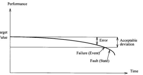
The relationship between error, failure and fault is illustrated in Figure2. The three terms are defined as follows [2].
1. Error is a discrepancy between a computed, observed or measured value or condition and
∗Correspondence to: T. S. Liu, Department of Mechanical
Engineer-ing, National Chiao Tung University, Hsinchu 30010, Taiwan, ROC. Email: [email protected]
the true, specified or theoretically correct value or condition.
2. Failure is an event when a required function is termi-nated (exceeding the acceptable limits).
3. Fault is the state characterized by inability to per-form a required function, excluding the inability dur-ing preventive maintenance or other planned actions or due to lack of external resources.
Based on the above statements, an error is not a failure and a fault is hence a state resulting from a failure. An error is sometimes referred to as an incipient failure [3]. Therefore PM action is taken when the system is still in an error condition, i.e. within acceptable deviation and before failure occurs. Thus, through the technique of PM, failure can be detected early.
There have been many methods proposed for early failure detection [4–6]. This study employs the Petri net modelling method coupled with parameter trend and fault tree analysis to perform early failure detection and isola-tion for PM. A fault diagnosis system for district heating and cooling facilities will be employed as an example to demonstrate the proposed Petri net method.
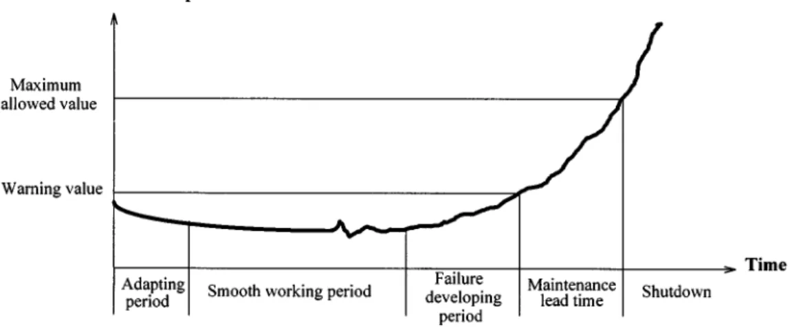
THRESHOLD AND WARNING VALUE A trend chart [7] is a chart that records the performance of a piece of equipment or a system by time. Methods for generating curves in a trend chart vary with different types of equipment, as depicted in Figure 3. Figure 4 shows a trend chart for a rotating machine. Trend charts are usually established by manufacturers when they run their tests in their laboratories to evaluate quality, reli-ability, maintainability and maintenance procedures. A threshold is a value used to judge whether an equipment failure occurs or not. It is prescribed as the measurement value that is taken just prior to or at the time of failure, i.e. the maximum allowed value in Figure4. Life testing is one method to obtain such data, and may be performed by field engineers or users.
CCC 0748–8017/98/050319–12$17.50 Received 30 September 1997
320 S. K. YANG AND T. S. LIU
Figure 1. Classification of maintenance
Figure 2. Error, failure and fault
Figure 3. Methods for generating curves in trend charts
Once the threshold has been determined, a margin of safety should be added to account for variations in early failure detection. The warning value in Figure4 is the edge of this margin. The safety margin can be determined by the requirement of lead time for PM or according to the physical properties and actual operating conditions of different systems. The lower the warning value is set,
the greater is the assurance that PM will be done prior to failure [1], though more labour manpower and cost will have to be expended. Three standard deviations is one possible choice in prescribing a warning value [8]. On the basis of failure thresholds and warning values, a control chart [1] can be constructed to conduct limit control, as illustrated in Figure5.
Failure detection can be carried out by comparing actual with nominal quantities, and fault isolation by comparing actual with fault quantities [9]. Consequently, an instrumentation system should be set up for the objec-tive of PM to acquire actual quantities at measurement points. In addition to being used for comparison, ac-quired quantities can be stored to establish a database for modifying predetermined failure thresholds and warning values. The performance of some systems depends on external conditions. For example, the output current of a power generator varies with the load, which changes with time during a day. Hence thresholds and warning values may be varied according to a scheduled scheme that accomplishes adaptive adjustment for those values. The situation is called ‘error’ in this paper whenever the
Figure 4. A trend chart for a rotating machine
Figure 5. A control chart
acquired quantity exceeds the prescribed warning value but falls within the high and low thresholds.
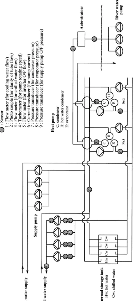
A fault diagnosis system for district heating and cool-ing facilities has been proposed [10]. This system is em-ployed as an example for early failure detection and isola-tion using the method proposed in this study. The system diagram is shown in Figure6. The facilities are composed of two heat pumps for producing heat, four storage tanks for storing hot and chilled water, two sets of supply pumps for supplying buildings with hot and chilled water respectively, and distribution pipes. The functions of the proposed fault diagnosis system for the facilities can be divided into two parts: reduced-capability diagnosis to prevent a failure and reduced-function diagnosis after a failure. They use the threshold of symptom detection to predict the fault time and a cause–effect tree diagram to find causes of faults. A trigger signal is generated which is a fault alarm or an upper or lower limit alarm once the measured data exceed a reference value. Reference values are presented in [10]. The value for condenser pressure, for example, is 0.1–0.7 kg cm−2, varying from September to December. The level of malfunction for this parameter is set at 15% up for the warning value and 20% up for the threshold. This system has been validated using real facilities.
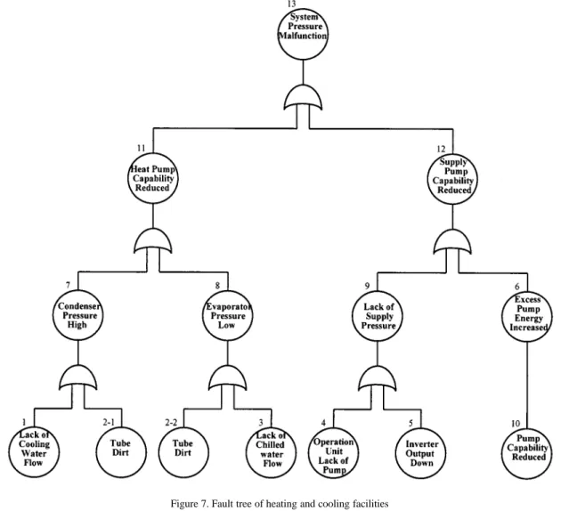
Figure7depicts the fault tree of this system. Events 1– 9 are measurable, whereas events 10–13 are phenomena which do not need to be measured. Since events 2-1 and 2-2 are the same event, they can be measured by the same sensor. In order to construct the Petri net dealing with system failure, nine sensors are selected to be installed at the associated test points depicted in the fault tree to acquire data. Sensor types, locations and associated sensing signals are depicted in Figure6.
PETRI NETS
A Petri net is a general-purpose mathematical tool for describing relations existing between conditions and events [11]. The basic symbols of Petri nets include [12]:
◦
place, drawn as a circle, denoting event— immediate transition, drawn as a thin bar, denoting event transfer with no delay time
— timed transition, drawn as a thick bar, denoting event
transfer with a period of delay time
↑ arc, drawn as an arrow, between places and
transi-tions
•
token, drawn as a dot, contained in places, denoting the data322 S. K. YANG AND T. S. LIU
◦
inhibitor arc, drawn as a line with a circle end,between places and transitions.
A transition is said to fire if input places satisfy an en-abled condition. Transition firing will remove one token from each input place and put one token into each output place [13]. The basic structures of the logic relations for Petri nets are listed in Figure8, where there are two types of input places for transition, namely specified and con-ditional. The former has a single output arc, whereas the latter has multiples. Tokens in a specified-type place have only one outgoing destination; that is, if the input place(s) holds a token, then the transition fires and gives the output place(s) a token. However, tokens in a conditional-type place have more than one outgoing path, which may lead the system to different situations. For the ‘TRANSFER OR’ Petri net in Figure8, whether Q or R takes over a token from P depends on conditions such as probability, extra action and self-condition of the place.
There are three types of transitions that are classified based on time [11]. Transitions with no time delay due to transition are called immediate transitions, while those that need a certain constant period of time for transition are called timed transitions. The third type is called a stochastic transition and is used for modelling a process with random time. Owing to the variety of Petri nets [11], it is a powerful tool for modelling flexible manufacturing systems [14,15], multilevel hierarchical systems [16,17], multiprocessor systems [18,19], etc. Besides, Petri nets are capable not only of simulation [20,21], reliability analysis [22] and failure monitoring [23] but also of dynamic behaviour observation [24] and activity predic-tion [25].
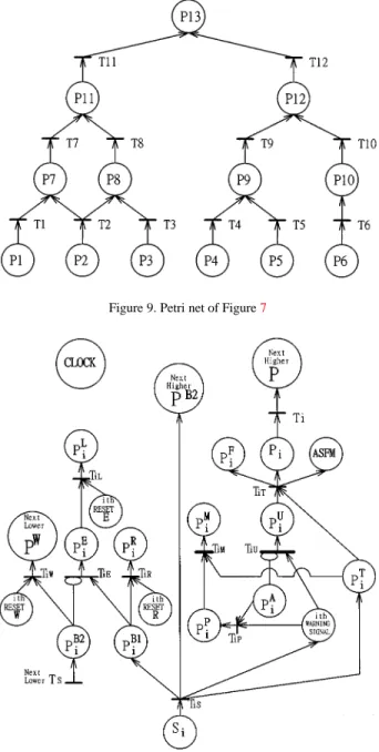
The proposed fault tree of the facilities shown in Fig-ure7can be transformed into the Petri net model shown in Figure9. Since events 2-1 and 2-2 in the fault tree depicted in Figure7 are the same, they have been com-bined into P2 in the Petri net depicted in Figure 9. As a result, each place in Figure9represents the associated fault event in Figure7.
EARLY FAILURE DETECTION AND ISOLATION ARRANGEMENT
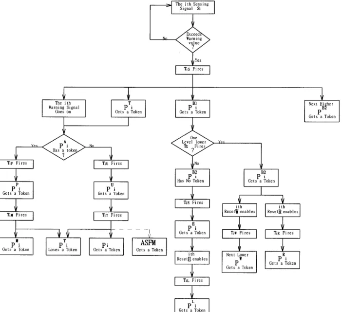
An early failure detection and isolation arrangement (EFDIA) is proposed in this paper. It is a hybrid Petri net [11] that includes three kinds of Petri nets: ordinary, inhibitor arc and timed. In Figure 9, each place with a monitor sensor, i.e. each of the nine measurement points in Figure6, will be equipped with an EFDIA that facilitates alarm, early failure detection, fault isolation, event count, system state description and automatic shutdown or regulation. EFDIA is shown in Figure10, where the symbols are defined as follows:
1. n: total number of sensing points 2. i : sequence number, 1≤ i ≤ n
3. M(P)k: marking of place P at state k, representing the token quantity of place P at state k, k= 1,2,3,... 4. Pi: i th place of Petri net; M(Pi) = 1 if Pi failure
occurs.
5. Ti: i th transition of Petri net, representing the time duration due to transition
6. Si: sensing signal for i th place; Si generates a to-ken such that M(Si) = 1 if the signal exceeds the prescribed warning value, i.e. an abnormal situation (error) occurs
7. Ti E: error transition of Pi; immediate transition 8. Ti L: error times log transition of Pi; immediate
tran-sition
9. Ti M: maintained transition, representing the transi-tional time from when the PM action for Pi is taken to when Pi is maintained, timed transition
10. Ti P: processing transition of Pi; immediate transition 11. Ti R: reset transition of Pi; immediate transition 12. Ti S: sensing transition of Pi; immediate transition 13. Ti T: transfer transition of Pi; immediate transition 14. Ti U: unprocessed transition of Pi, representing the
transitional time from when the i th WARNING SIG-NAL appears to when Pi failure occurs; timed tran-sition
15. Ti W: warning times log transition of next lower level PW; immediate transition
16. PiA: PM action taken place for Pi; PiA generates a token such that M(PiA) = 1 if the PM action for Pi is taken
17. PiB j: j th buffer place of Pi, for tokens to stay tem-porarily, j = 1,...,x; x is the number of input arcs for Pi
18. PE
i : error indication place of Pi; M(PiE) = 1 after Ti E fires if the M(Si) = 1 situation is generated by Pi itself but not aroused by lower-level places (for fault isolation)
19. PiF: failure counter place of Pi; M(PiF) represents the failure times log number of Pi; M(PiF) increases by one when Pifailure occurs
20. PiL: error counter place of Pi; M(PiL) represents the error times log number of Pi; M(PiL) increases by one when Pierror occurs
21. PiM: maintenance counter place of Pi; M(PiM) rep-resents the maintenance times log number of Pi; M(PiM) increases by one when the M(Si) = 1 sit-uation is maintained
22. PiP: processing place of Pi, representing Pi in the being maintained situation
23. PR
i : reset counter place of Pi; M(PiR) represents the warning times log number of Pi that are aroused by lower-level places, i.e. the reset times of the i th RESET R; M(PiR) increases by one when the ith RESET R is triggered
24. PiT: transitional place of Pi, representing a transi-tional state inserted between Si and Pi, of duration Ti Splus Ti T, which is the original path from Sito Pi without EFDIA constructed
25. PiU: unprocessed place of Pi, representing the error of Pinot corrected
26. PiW: warning counter place of Pi; M(PiW) represents the warning times log number of Pi no matter from where warning cause arises; M(PW
i ) increases by one when the i th RESET W is triggered
27. i th RESET E: reset E place of Pi, representing a reset signal for PE
324 S. K. YANG AND T. S. LIU
Figure 7. Fault tree of heating and cooling facilities
Figure 8. Basic structures of logic relations for Petri nets
28. i th RESET R: reset R place of Pi, representing a reset signal for PiR; generates a token when it is triggered
29. i th RESET W: reset W place of Pi, representing a reset signal for PiB; generates a token when it is triggered; the number of the i th RESET W should equal number of inhibitor arcs of transition Ti E 30. ASFM: automatic shutdown or feedback
mechanism; for instance, an air-conditioning or ventilation system is a feedback mechanism for an over temperature module
31. i th WARNING SIGNAL: warning signal place for Pi
32. CLOCK: a clock is embedded to record the time of event occurrence
The operational steps for EFDIA are described as follows. 1. Transition Ti S fires if Si exceeds the prescribed warning value. Subsequently, each of PiB1, i th WARNING SIGNAL, PiT and next higher PB2 obtains a token. As defined in the previous paragraph, M(P) is the marking of place P. Thus M(PT
i ) = 1 represents this Si monitored subsystem (module) at a transitional state. Similarly, M(i th WARNING SIGNAL) = 1 represents that the ith
Figure 9. Petri net of Figure7
Figure 10. Early failure detection and isolation arrangement (EFDIA)
WARNING SIGNAL goes on, which may be a light, a beep or some other form, to indicate that Si exceeds the prescribed warning value.
2. There are two paths to follow.
(a) Ti Pfires if PiAgenerates a token, i.e. PM action is taken. The tokens in PiA and the i th WARN-ING SIGNAL move to PiP, i.e. the subsystem (module) is being maintained. Otherwise, Ti U fires if PiAdoes not generate a token during the transition time of Ti U, such that PiU acquires a token.
(b) Ti Efires if PiB2has no token, i.e. this error is not caused by the next lower subsystem (module) but by the i th-level subsystem (module) itself, such that PiEobtains a token. On the other hand, if PiB2 holds a token, i.e. this error results from the next lower subsystem (module), then Ti E does not fire, such that the token from Si will be held in PiB1. The error is hence isolated.
3. There are again two paths to follow.
(a) Ti Mfires if the PM action is finished, such that the tokens in PiPand in PiTmove to PiM, i.e. this error has been corrected. Otherwise, Ti T fires if PiU obtains a token resulting from the firing of Ti U, i.e. PM action was not taken in time, such that tokens in PiUand PiTmove to Pi, i.e. Pi failure occurs. As a consequence, both PiF and ASFM also obtain a token. Accordingly, the failure times log number increases by one and the ASFM is triggered. This mechanism can be optional for different systems.
(b) Ti Lfires if PiEholds a token and the i th RESET E is triggered, such that PiLobtains a token, i.e. the error times log number of Pi increases by one. Otherwise, the token in buffer place PiB1 will move to PiRwhen Ti Rfires by triggering the i th RESET R, i.e. this error is not caused by Pi and the reset times log number of Pi increases
326 S. K. YANG AND T. S. LIU
Figure 11. Flow chart of EFDIA
by one. Similarly, the i th RESET W triggers to fire Ti Wsuch that the token in the other buffer place, PiB2, moves to the next lower PW, i.e. the warning times log number of the next lower PW increases by one.
Conventionally, a flow chart is an easier representation for understanding the operational steps. Therefore the above descriptions are summarized into a flowchart for clarity, as shown in Figure11.
EFDIA is composed of several small arrangements, each of which has a specific function.
1. Reset. The i th RESET E and PiE together with Ti L form a logic AND relation. The i th RESET E gen-erates a token whenever this reset button has been triggered, so as to fire Ti Land remove a token from PE
i to PiLwhenever PiE holds a token and needs to be reset. In a similar manner, the i th RESET R and i th RESET W are designed to reset PB1
i and PiB2 respectively.
2. Inhibition. Both Ti E and Ti U are transitions with an inhibitor arc. This arrangement is designed to inhibit the firing of Ti Eand Ti U whenever the place where the inhibitor arc is connected, i.e. PiB2and PiA respectively, holds a token.
3. Conditional place. Any place that has more than one outgoing arc is called a conditional place. Tokens contained in a conditional place will move to an output place through the transition which is firstly enabled among all the output transitions of the tran-sitional places. A conditional place models a condi-tional state of a system or process. In EFDIA, PiA, PiB1, PiB2, PiT and the i th WARNING SIGNAL are conditional places.
4. Counter. PiF, PiL, PiM, PiRand PiWperform as coun-ters to accumulate occurrence times of associated events.
5. Event flag. Several places are designed as event flags. Each of them represents an associated event once the marking of the place becomes unity.
(b) PE
i denotes the error located at the i th place. (c) PT
i denotes the i th place at a transitional state. (d) The i th WARNING SIGNAL denotes the i th
monitored signal exceeding the warning value. (e) ASFM means the automatic shutdown function
or feedback mechanism is triggered.
PROPERTIES OF EFDIA
This section presents the capabilities of EFDIA and the invariants derived from EFDIA.
Capabilities
1. Alarm. EFDIA provides alarm capability whenever an over-warning-value situation occurs, by triggering the i th WARNING SIGNAL for the associated place. 2. Early failure detection. EFDIA is capable of early failure detection, since the alarm function operates whenever the acquired signal exceeds a prescribed warning value but not the failure threshold. This means that the abnormal situation is detected before failure occurs. As shown in Figure5, the lead time of early detection can be obtained by extrapolating the curve in a control chart with a line slope that is constructed by the last two sampled points on the curve [10]. The lead time is the period between the time point where the warning value is exceeded and the intersection of the extended line and time axis. 3. Fault isolation. The cause(s) of malfunction of a
system can be located anywhere within the system. However, since malfunction causes are constrained by the logic relations of the fault tree, they can be isolated by the inhibit transition Ti E via the indica-tion of the event flag PiE. The error is located at the i th place if M(PiE) = 1. Otherwise, the error of the i th place arises from the lower-level place(s) even if the i th WARNING SIGNAL appears.
4. Event count. All the counters designated in EFDIA record the associated occurrence times of events. By incorporating a time clock, the associated rates can be obtained at the same time. The following items can be derived from EFDIA:
(a) failure rate of the i th place: M(PF i )/t (b) error rate of the i th place: M(PiL)/t (c) maintenance rate of the i th place: M(PiM)/t (d) alarm rate of the i th place: M(PiW)/t. From these rates, two advantages can be obtained.
(a) If the i th subsystem is maintained whenever an error is detected, the failure rate of the i th place can be minimized such that the system reliability is promoted.
(b) All the rates can be recorded as historical data so as to perform statistical prediction for system failure (by failure rate and error rate), and the time needed for maintenance (by maintenance rate) of each subsystem can be derived.
5. System state description. The system state is clearly visible by the indication of every place in EFDIA. The following parameters are defined to account for
the system state:
(a) Mk: marking of the Petri net at state k, Mk= [M(P1), M(P2),..., M(Pn)]T
(b) Sk: sensing signal matrix at state k,
Sk= [M(S1), M(S2),..., M(Sn)]T
(c) Lk: maintenance log matrix at state k, Lk = [M(P1M), M(P2M),..., M(PnM)]T
(d) Fk: failure times log matrix at state k, Fk = [M(P1F), M(P2F),..., M(PnF)]T
(e) Ek: error indication matrix at state k,
Ek = [M(P1E), M(P2E),..., M(PnE)]T; the i th entry indicates that the error is located at the i th place if the i th entry value is unity.
6. Auto shutdown or regulation. Automatic shutdown or regulation capability can be provided by EFDIA through triggering the ASFM place.
7. Time recording. The time at which each event occurs can be recorded by the embedded CLOCK. This is required for failure analysis.
Invariants
According to the properties of EFDIA, the following invariants can be derived:
1. M(PiL)k + M(PiR)k = M(PiW)k. The number of warning signals for the i th place at state k is equal to the summation of the error times log number and the reset times log number at state k for the i th place. 2. M(PF
i )k + M(PiM)k = M(PiW)k. For the ith place at state k, failure times plus maintenance times equal the warning times log number.
3. At basic places, M(PR)k = 0 and M(PL)k = M(PW)k. Since there is no place lower than basic places, the error times log number and the warning times log number are equal at basic places.
4. M(PiP)k + M(PiU)k = 1. Since the conditions that an error place is maintained and not maintained are mutually exclusive, at state k either the marking for PiPor that for PiUis unity.
EXAMPLE
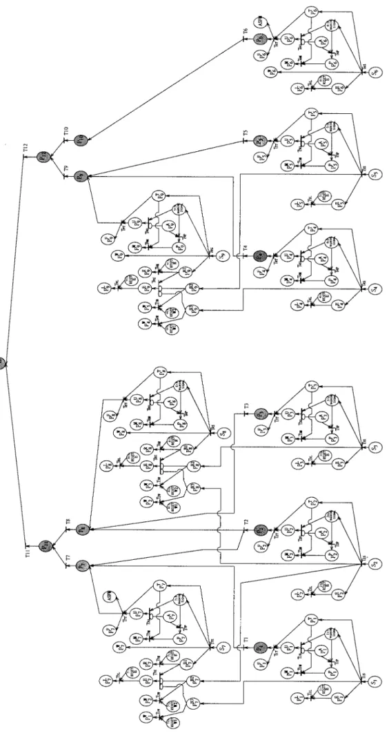
The Petri net for the heating and cooling facilities en-dowed with EFDIA is shown in Figure12. It is a result of appending an EFDIA to each place with a monitor sensor in Figure 9, i.e. P1 to P9. The logic relations among all places in Figure9are still retained in Figure12. At basic places, i.e. P1 to P6, the function for testing whether the error cause is from the next lower place or not becomes unnecessary. The following two situations are used to demonstrate the function of EFDIA in the employed system.
1. Suppose the monitored signal for cooling water flow, i.e. S1 in Figure 12, exceeds the prescribed warn-ing value. Subsequently, T1S fires such that the 1st WARNING SIGNAL goes on and each of P1T, P7B3 and PE
1 obtains a token. M(P1T) = 1 represents the cooling water flow rate that is in an error situation and it is a transitional state between normal and faulty. There is a lead time from then until P1failure
328 S. K. YANG AND T. S. LIU
really happens. If the PM action takes place during the lead time, then PA
1 generates a token such that T1Pfires so as to make the tokens in P1Aand the 1st WARNING SIGNAL move to P1P. The subsystem is being maintained and the 1st WARNING SIGNAL goes off at this moment. T1M fires if the PM action is finished. Subsequently, the tokens in P1P and P1T move to P1M, i.e. this error has been corrected. The marking of P1M, i.e. the maintenance times log num-ber for P1, increases by one. On the other hand, if the PM action does not take place in time, then T1U fires such that P1Uobtains a token. Consequently, the tokens in P1Uand P1Tmove to P1. Hence P1failure occurs. At the same time, P1Fobtains a token, i.e. the failure times log number increases by one. Because of the logic relation between P1 and P7, the mon-itored signal for P7, i.e. S7, exceeds the prescribed warning value due to P1failure. Accordingly, the 7th WARNING SIGNAL goes on and each of P7T, P7B1 and P7W, obtains a token. T7Eis inhibited by the token in P7B3, such that the tokens in P7B1and P7B3move to P7Rand P1Wafter triggering the 7th RESET R and 7th RESET W1 respectively. Hence this error is located at P1, whereas M(P7L) does not increase.
2. Suppose the monitored signal for condenser pres-sure, i.e. S7, exceeds the prescribed warning value spontaneously while both S1 and S2 are at normal condition. As a result, T7S fires such that the 7th WARNING SIGNAL goes on. Simultaneously, each of PT
7, P7B1 and P W
7 obtains a token. In a similar manner, as S1exceeds the prescribed warning value, M(P7M) increases by one if the PM action for P7 takes place in time. Otherwise, P7 failure occurs such that M(P7F) increases by one. However, since P7B2and P7B3are both empty, T7Efires such that P7E obtains a token. As a result, M(P7L), i.e. the error times log number for P7, increases by one.
ASFM is to prevent higher-level fault or system break-down from happening by automatic shutbreak-down or regula-tion. It should be incorporated with the places that may cause safety problems in a Petri net. In this example it can be triggered by either P6or P7failure, i.e. excess pump energy increased or condenser pressure high.
CONCLUSIONS
This paper has presented an early failure detection and isolation scheme for PM via the heating and cooling facilities example, by using a hybrid Petri net modelling method coupled with parameter trend and fault tree anal-ysis. The Petri net dealing with system failure has to be constructed beforehand. The next task is to obtain trend charts for all fault places in the Petri net in or-der to prescribe thresholds and allowable margins. With these prerequisites the present method can be applied to any system. The proposed Petri net approach can not only achieve early failure detection and isolation for fault diagnosis but also facilitates event count, system state description and automatic shutdown or regulation. These capabilities can be very useful for health monitoring and preventive maintenance of a system.
REFERENCES
1. J. D. Patton Jr, Preventive Maintenance, Instrument Society of America, New York, 1983.
2. IEC 50(191), International Electrotechnical Vocabulary (IEV), Chap. 191, Dependability and Quality of Service, International Elec-trotechnical Commission, Geneva, 1990.
3. M. Rausand and K. Oien, ‘The basic concept of failure analysis’, Reliab. Eng. Syst. Safety, 53, 73–83 (1996).
4. W. J. Wang and P. D. McFadden, ‘Early detection of gear failure by vibration analysis—I. Calculation of the time–frequency distri-bution’, Mech. Syst. Signal Process., 7(3), 193–203 (1993). 5. W. J. Wang and P. D. McFadden, ‘Early detection of gear failure
by vibration analysis—II. Interpretation of the time–frequency dis-tribution using image processing techniques’, Mech. Syst. Signal Process., 7(3), 205–215 (1993).
6. R. Isermann, ‘Process fault detection based on modeling and esti-mation methods—a survey’, Automatica, 20(4), 387–404 (1984). 7. G. G. Barna, ‘Automatic problem detection and documentation for
a plasma etch reactor’, IEEE Trans. Semicond. Manuf., SM-5(1), 56–59 (1992).
8. S. S. Rao, Reliability-Based Design, McGraw-Hill, New York, 1992. 9. A. Baccigalupi, A. Bernieri and A. Pietrosanto, ‘A digital-signal-processor-based measurement system for on-line fault detection’, IEEE Trans. Instrum. Meas., IM-46(3), 731–736 (1997).
10. T. Kumamaru, T. Utsunomiya and Y. Yamada, ‘A fault diagnosis system for district heating and cooling facilities’, Proc. IECON ’91, Int. Conf. on Industrial Electronics, Control, and Instrumentation, 1991, pp. 131–136.
11. R. David and H. Alla, ‘Petri nets for modeling of dynamic systems—a survey’, Automatica, 30(2), 175–202 (1994).
12. G. S. Hura and J. W. Atwood, ‘The use of Petri nets to analyze coherent fault trees’, IEEE Trans. Reliab., REL-37(5), 469–474 (1988).
13. W. G. Schneeweiss, ‘Mean time to first failure of repairable systems with one cold spare’, IEEE Trans. Reliab., REL-44(4), 567–574 (1995).
14. M. C. Zhou, H. S. Chiu and H. H. Xiong, ‘Petri net scheduling of FMS using branch and bound method’, Proc. IEEE IECON, 21st Int. Conf. on Industrial Electronics, Control, and Instrumentation, 1995, pp. 211–216.
15. R. Hilal and P. Ladet, ‘Modelling, control, and simulation of flex-ible manufacturing systems through the use of synchronous Petri nets’, Proc. IECON ’93, Int. Conf. on Industrial Electronics, Con-trol, and Instrumentation, 1993, pp. 559–563.
16. H. Murakoshi, T. Kondo and Y. Dohi, ‘Hardware architecture for hi-erarchical control of large Petri net’, Proc. IECON ’93, Int. Conf. on Industrial Electronics, Control, and Instrumentation, 1993, pp. 115– 120.
17. P. Esteban and M. Courvoisier, ‘Multilevel hierarchical control ap-plied to a demonstration flexible assembly cell’, Proc. IECON ’91, Int. Conf. on Industrial Electronics, Control, and Instrumentation, 1991, pp. 878–883.
18. F. Anzai, N. Kawahara and T. Takei, ‘Hardware implementation of a multiprocessor system controlled by Petri nets’, Proc. IECON ’93, Int. Conf. on Industrial Electronics, Control, and Instrumentation, 1993, pp. 121–126.
19. H. Murakoshi, M. Sugiyama, G. Ding and T. Oumi, ‘A high speed programmable controller based on Petri net’, Proc. IECON ’91, Int. Conf. on Industrial Electronics, Control, and Instrumentation, 1993, pp. 1966–1971.
20. J.-F. Ereau and M. Saleman, ‘Modeling and simulation of a satellite constellation based on Petri nets’, Proc. IEEE Ann. Reliability and Maintainability Symp., 1996, pp. 66–72.
21. H. Takami and M. Araki, ‘Simulation-based scheduling package using generalized Petri net models’, Proc. IECON ’93, Int. Conf. on Industrial Electronics, Control, and Instrumentation, 1993, pp. 451– 456.
22. K. Barkaoui, G. Florin, C. Fraize and B. Lemaire, ‘Reliability anal-ysis of nonrepairable systems using stochastic Petri nets’, Eigh-teenth Int. Symp. on Fault-Tolerant Computing. Digest of Papers. FTCS-18, 1988, pp. 90–95.
23. A. Chaillet, M. Combacau and M. Courvoisier, ‘Specification of FMS real-time control based on Petri nets with objects and process failure monitoring’, Proc. IECON ’93, Int. Conf. on Industrial Elec-tronics, Control, and Instrumentation, 1993, pp. 144–149. 24. S. K. Yang and T. S. Liu, ‘Failure analysis for an airbag inflator by
Petri nets’, Qual. Reliab. Eng. Int., 13, 139–151 (1997).
25. Y. Manabe, M. Hattori, S. Tadokoro and T. Takamori, ‘A model of human actions by a Petri net and prediction of human acts’, Trans. Jpn. Soc. Mech. Eng., 63, 287–294 (1997).
330 S. K. YANG AND T. S. LIU
Authors’ biographies:
S. K. Yang was born in Taiwan. He received his BS and MS in automatic control engineering from Feng Chia University in 1982 and 1985 respectively. From 1985 to 1991 he was an assistant researcher and system engineer in the Flight Test Group, Aeronautic Research Laboratory, Chung Shan Institute of Science and Technology. Since 1991 he has been an instructor in the Department of Mechanical Engineering, Chin Yi Institute of Technology. Since 1994 he has been a PhD student majoring in Mechanical Engineering at National Chiao
Tung University. His research interests are in reliability, data acquisition and automatic control.
T. S. Liu received his BS from National Taiwan University in 1979 and MS and PhD from the University of Iowa, USA in 1982 and 1986 respectively, all in mechanical engineering. Since 1987 he has been with National Chiao Tung University, where he is currently a professor. From 1991 to 1992 he was a visiting researcher in the Institute of Precision Engineering, Tokyo Institute of Technology, Japan. His current research in-terests include reliability, design, and motion control.