Scheduling algorithm for nonpreemptive multiprocessor tasks

(1)

0898-1221(94)00129-4 0898-1221/94 $7.00 + 0.00

Scheduling Algorithm for Nonpreemptive

Multiprocessor Tasks

J.-F.

LIN AND S.-J. CHEN Department of Electrical Engineering

National Taiwan University Taipei, Taiwan 106, R.O.C. (Received May 1993; accepted June 1993)

Abstract-This paper considers the problem of scheduling nonpreemptive multiprocessor tasks in a homogeneous system of processors. The problem proposed in this paper is different from the conventional scheduling problem, where each task requires only “one” processor whenever it is in processing. In our multiprocessor task scheduling problem, tasks can require more than one processor at a time for their processing, that is, tasks in our problem require simultaneously “j” arbitrary processors when they start to be processed, where 1 5 j 5 k and k is a fixed number. Though multiprocessor tanks considered in this paper are assumed to be independent, i.e., the precedence relation does not exist among them, such a problem of scheduling nonpreemptive multiprocessor tasks is NP-complete. Therefore, a heuristic algorithm is investigated for this kind of problem and the worst performance bounds of the algorithm are also derived.

Keywords-Multiprocessor task, Largest processing time first scheduling rule, Performance bound.

1. INTRODUCTION

An assumption in conventional scheduling problems [l-3] is that each task is processed on only “one processor” at a time. The assumption was modified by Blazewicz, Drabowski, and Weglarz [4,5] such that different tasks are to be processed on a “different number of processors.” They considered a set T of n independent tasks which are to be processed on a set of m identical processors P = {PI, P2, . . . , Pm}. This set of n independent tasks, T, can be decomposed into k subsets,suchthat’IT=T1UT2U~~~UTICwhereT1={T~,T~,...,T~,},T2={T~,T~,...,T~~},

. . . , Tk = {Tf, Tt, . . . , T&} and n = ni + nz + ‘. . + nk. That is, each task in T1 requires one arbitrary processor for its processing and each task in Tj requires j arbitrary processors simultaneously for its processing. In summary, for a task T!, i = 1,2,. . . , nj, exactly j arbitrary processors (here, j can be 1 to k) are allocated to it during a period of t{ , which is the computation time of task T/. Note that in the defined multiprocessor task scheduling problem, a schedule is feasible if each task T: can be exactly processed by j processors simultaneously, and the performance of a feasible schedule is measured by its schedule length such that a feasible schedule is called an optimal schedule if it is of minimum schedule length.

In solving the above problem, polynomial time algorithms were proposed by Blazewicz, Dra- bowski, and Weglarz [5]. But these optimal algorithms were only designed for two constrained cases of independent multiprocessor task schedulings: one case was that multiprocessor tasks are with “unit” computation time; the other one was that multiprocessor tasks are with arbitrary computation time, but they need to be “preemptive.”

Typeset by A@-‘I)$ 85

(2)

In this paper, we will pay attention to the problem of scheduling independent “nonpreemptive” multiprocessor tasks with “arbitrary” computation times, which is NP-complete because the scheduling of the independent nonpreemptive tasks with arbitrary computation time of T’, a special case of this problem, was already known to be NP-complete [1,3]. Therefore, we are interested in polynomial time approximation algorithms, that is, we try to get an approximate solution using heuristic algorithms. We say that a heuristic algorithm has a performance bound P if (SHISO) 5 P f or all problem instances, where SH and So denote the heuristic schedule

length and the optimal schedule length, respectively.

Remember that the Largest Processing Time first scheduling rule (LPT) was a well-known rule for the conventional scheduling of independent tasks nonpreemptively on identical processors. In other words, the LPT is a rule for scheduling those independent nonpreemptive tasks T1 in a homogeneous system of processors. The principle of LPT is that whenever “a” processor becomes free, select a task whose computation time is the largest of those not yet assigned tasks to assign to it. Graham analyzed [2] that the ratio of the LPT and the optimal schedule lengths is bounded by (4 - &), where m is the number of processors in a system. Based on the principle of LPT, we develop a heuristic algorithm for the problem of scheduling independent nonpreemptive multiprocessor tasks and derive the performance bounds for two cases of this algorithm.

The remainder of this paper is organized as follows: The basic concept of Largest-Processing- Time first scheduling rule is presented and based on this LPT rule, the algorithm and the perfor- mance bound of scheduling one set of independent nonpreemptive multiprocessor tasks, say Tj, are derived in Section 2. Section 3 illustrates how the derived algorithm can be extended to schedule the complete task set T. The performance bound of this heuristic algorithm is proved to be bounded by (Z/C - (k(rC + 1)/6m]) for th e case in which both the number of processors in a system and the number of processors required by each task are arbitrary. Furthermore, the performance bound for a special case, in which both of the number of processors in a system and the number of processors required by each task are power of 2, is shown to become (2 - 6). Finally, some concluding remarks are given in Section 4.

2. THE LARGEST PROCESSING

TIME

FIRST SCHEDULING

RULE

The largest processing time first scheduling rule (LPT) is a popular heuristic algorithm for the conventional nonpreemptive scheduling of independent tasks with arbitrary computation times. This LPT rule was first proposed by Graham in [2] to nonpreemptively schedule independent tasks which require only “one” processor whenever they are in processing. A formal description of LPT is given as follows:

ALGORITHM LPT. Begin

Input task set T1;

While (there exist tasks unassigned in T’) do Begin

If (there exists a free processor Pa, Q = 1,2,. . . = 1,2,. . . , m) then Begin

Assign task Tt whose computation time is the largest among those tasks in T1 to processor Pa; Remove task Tt from T1;

Endif EndWhile

End

From the above algorithm, it is obvious that tasks have to be sorted in nonincreasing order of their computation times. Then, tasks are assigned, according to this sorting sequence, to the first free processor they meet. Graham has shown that the performance bound of LPT is ($ - &).

(3)

Scheduling Algorithm 87 That is, let SH denote the schedule length of a corresponding LPT schedule and So denote the schedule length of an optimal schedule. Then, (SH/SO) I ($ - &-), where m is the number of processors in a system. A simple example will be given to illustrate the above result.

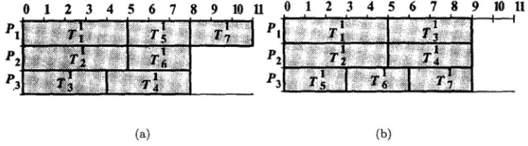
EXAMPLE 1, Assume that there are 7 tasks T;, Ti, Ti, Ti, T:, Ti, and T; submitted to a system of 3 identical processors. The computation times of these tasks are 5, 5, 4, 4, 3, 3, and 3, respectively. Figures 1 (a) and (b) illustrate the LPT schedule and an optimal schedule, respectively.

From the figure, we observe that 2 = y = 4 - &. I

(4

(b)

Figure 1. The LPT schedule and an optimal schedule

In the following, we will apply the concept of LPT [2] to the nonpreemptive scheduling of independent mutiprocessor task set Tj, where each task in Tj requires exactly j arbitrary processors for its processing, and derive its performance bound.

THEOREM 1. The performance bound of scheduling one set of independent nonpreemptive mul-

tiprocessor tasks Tj = {T[ , Tl , . . . , Ti, T$}, based on the rule of LPT, on m identical processor

systems is bounded by ($ -

_{&-) ,}

where j 5 m and cj = LT].

PROOF. Assume that the independent nonpreemptive multiprocessor tasks in Tj = {T!‘, Ti,

.

. . ,

Ti.} have been sorted in nonincreasing order of their computation times. By using the LPT ru;e, tasks in Tj = {T;, Ti,. . . , Ti .} are assigned to a system of m identical processors. Let Sk and Sh denote the LPT schedule length and the optimal schedule length of the task subset Tj, respectively.

We can assume that m = (cj x j) +rj, where cj and rj are positive integers. If Tj # 0, then the m-processor system can be seen as a (cj x j)-processor system, because the number of processors can be used by the set of task Tj is (cj x j) and there would always exist rj free processors. Thus,

(1) (2)

we can consider this system as a (cj x j)-processor or an (m - rj)-processor system. If S$ = S&, then it is obvious that the theorem holds.

For the case that S& > S&, there exists a largest integer XC~, such that the ~:j longest tasks of the task set Tj are assigned to (cj x j) identical processors by the LPT scheduling rule with an optimal schedule. Then, if the longest computation time of the remaining (nj - zj) unassigned tasks is T = r TM,F~, {ti}, where t{ is the computation time of task

T/, it is obvious that the above (cj 5( jj drocessors cannot be idle before time (Sk - 7).

Hence,

j 2 ti 2 (m - Tj) X (S& - T) + (j X T). _(2.1) i=l

From equation (2.1), we have equation (2.2):

(4)

With (m - rj) = (cj x j), and from equation (2.2), we derive equation (2.3):

(2.3) Since there are at least (zj + 1) tasks whose computation time are greater than or equal to 7, the (m - r-j) processors must be assigned with at least of these (z~j + 1) longest tasks. This imdies:

s&‘(1+[$

(2.4)

From equation (2.3) and (2.4), we can derive equation (2.5) which is the performance bound equation of the task set TJ on an m identical processor system.

(2.5)

Since xj must be greater than cj (otherwise it would be an optimal schedule), the worst case occurs when [(xj)/(cj)l = 2. Th ere ore, f the worst performance bound is ($-&). I

The following simple example will show that the above performance bound is tight.

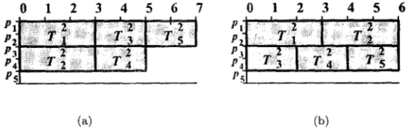
EXAMPLE 2. Consider a system in which there are 5 identical processors, m = 5, and a set of tasks T2 = {T&T&T;, T:, T,2} are submitted to this system. The computation times of Tf, T:, Tz, T:, and Tz are 3, 3, 2, 2, and 2, respectively. The LPT schedule and an optimal schedule are illustrated in Figures 2 (a) and (b), respectively. Since m = 5 and j = 2, we can calculate that c2 = 151 = 2. Thus, we conclude that the performance bound (Ss)/(Sz) = 5 = (i - &) is

tight. I 0 1 2 3 4 5 G 7 0123456 P P P P P P P P P P

(4

(b)

Figure 2. The LPT schedule and an optimal schedule of task set T2

3. HEURISTIC

ALGORITHM

In this section, we will propose a heuristic algorithm for the problem of scheduling independent nonpreemptive multiprocessor tasks which is based on the concept of LPT rule. Before giving a formal description of our heuristic algorithm, the multiprocessor task scheduling problem is stated as follows.

Consider a set of n independent nonpreemptive tasks, T, to be processed on a set of m identical processors P = {PI, Pz, . . , Pm}. Suppose that this set of n independent multiprocessor tasks can be decomposed into k task subsets T1 = {Tt,Ti,. . . ,Til}, T2 = {Tf,T$, . . . ,T&}, . . . , Tk = {T~,T$,... ,T,k,}suchthat.t=T1UT2U.~.UTk,,=,1+,2+...+~k,andeachtask

Tj, i= 1,2 ,..., nj, requires “j” arbitrary processors at a time for its processing during a period of time t{, which is the computation time of task T/. Here, tasks are said to be independent which means that there are no precedence constraints among them. Scheduling of tasks is termed nonpreemptive if a task cannot be interrupted once it has begun execution; that is, it must be

(5)

Scheduling Algorithm 89 allowed to run to completion. The problem of scheduling independent nonpreemptive tasks is an NP-complete problem. In this section, we will devote our attention to developing a heuristic algorithm for such a problem and deriving the performance bounds for two cases of problems: one is that both the number of processors in systems and the number of processors required by each task are arbitrary; the other one is that both the number of processors in systems and the number of processors required by each task are power of 2.

The formal description of our scheduling algorithm is illustrated below: HEURISTIC ALGORITHM.

Begin

Input task set T;

Divide task set T into k task subsets T1, T2, . . . , and Tk;

timefree = 0 /* Initialize that processors were free at time 0. */ For j = k downto I do

Sort tasks in Tj in nonincreasing order; Begin

For i = 1 to nj do /* Assume that there are nj tasks in Tj. */ Begin

While (there do not exist j free processors at time timefree) do Begin

timefree = timefree + 1; EndWhile

Assign task Ti to these j free processors; EndFor

EndFor End

In the above algorithm, the task set T is first divided into k task subsets T1, T2,. . . , and Tk. Then, the tasks in each task subset are scheduled according to the LPT scheduling rule. The major policy of our algorithm is that the more number of processors a task requires the earlier our scheduling algorithm takes it into consideration.

In the following theorems, we will show that the performance bounds of our heuristic algorithm for the above two cases of problems.

THEOREM 2. The performance bound of our scheduling algorithms is bounded by

( 4 k -

v)

,

in the case that the number of processors in a system and the number of processors required by each task are arbitrary.

PROOF. Let SH and So represent, respectively, the heuristic schedule length and the optimal schedule length of the task set T. Since SH = S& U S& U . . . U SfEI, where S$ represents the schedule length of the task subset Tj using the LPT scheduling rule on an m-processor system, for j = 1,2, . . . , k. Therefore,

because S& < So, where S& represents the optimal schedule length of any task subset Tj on an m-processor system for j = 1,2,. . . , k.

(6)

a

In the following, we will consider the case in which both of the number of processors in a system and the number of processors required by each task are power of 2. Such a case can be found in hypercube systems. The performance bound of our heuristic algorithm in this case is shown in Theorem 3.

LEMMA 1.

The number of free processors in a system would always be a multiple of the number

of processors required by a task which is the next to be scheduled.

PROOF.

When both of the number of processors in a system and the number of processors

required by each task are power of 2, we can assume that the number of processors in the system is 2 log, m and the task sets are T2h, T2h-’ , . . . , T’, where h 5 log, m. It is clear that if { 21% m - c;=,(ui x 2”,} > 0, then it must be a multiple of 2”, where 0 5 u 5 h, and ai is either a positive integer or a zero. The policy of our algorithm is the more number of processors a task requires, the earlier it will be scheduled. Thus, it is obvious that the lemma holds. I

LEMMA 2.

If the task T$ is finished at time SH, then there would be no processors idle before

(SH - t”,), where q is an integer of power of 2 and q 5 m, 1 5 x <_ nq, t$ is the computation time of task T,Q, and SH is the schedule length of our heuristic algorithm.

PROOF.

We will prove this lemma by contradiction. By Lemma 1, if there were some processors

idle before (SH - t!$), there must be enough free processors for the task T$. Then, T,” should be scheduled before (SH - tQ,). This leads to a contradiction. Therefore, there would be no processor

idle before (SH - tz). I

THEOREM 3.

The performance bound of our heuristic algorithm is bounded by (2 - A), if both

the number of processors in a system and the number of processors required by each task are power of 2, where m is the number of processors in a system.

PROOF.

Assume that the task T,” is finished at time SH, where q < k 5 m, x 5 ngr and SH is

the schedule length of the task set T by our heuristic algorithm. By Lemma 2, we can get:

(m x SH) 5

k

2 (j

x

t{) +

(m - 1)

x

tz

j=l i=l

6

3 (j

x

6) +

(m _ 1)

j SH < j=li=l

m m x t;.

Since ([Cf=, CYLi(j x t:)] /m) _ < So and ti 5 So, where So denotes the optimal schedule length of the task set T, for j = 1,2,4,. . . , k, i =

1,2,.

. . , nj.

So

(7)

Scheduling Algorithm 91

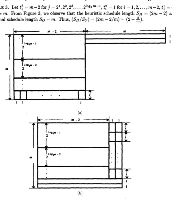
We will give a simple example to show that the performance bound is almost tight.

EXAMPLES. Letti =m-2forj=21,22,23

,..., 2’0~~m-1,t~=1fori=1,2

,..., m-2,t#=m,

and

t; = m.

From Figure 3, we observe that the heuristic schedule length SH = (2m - 2) and

an optimal schedule length So = m. Thus, (&/SO)

= (2m - 2/m) = (2 - 2).

_I

D) -2

-L

m

l

2 . .

I,

lOOl”-2 In

2 L

“_

I

. . . I

9

2 1 1 1 1 1

(4

t

nr -2

.I

1 a 9 2 I

2

OBzrn - I

f

(b)

Figure 3. The heuristic schedule and an optimal schedule.

4. CONCLUSIONS

In this paper, we propose a heuristics algorithm for the problem of scheduling independent

nonpreemptive

multiprocessor

tasks and show that its performance

bound is bounded by

(4k - [k(k + 1)/6

₃

m 1) in case the number of processors in the system and the number of proces-

sors required by each task are arbitrary. Besides, we also derive that the performance bound of

our scheduling algorithm is bounded by (2 - A), an almost tight performance bound, if both of

the number of processors in a system and the number of processors required by each task are

power of 2.

Since the performance bound of scheduling nonpreemptive multiprocessor tasks for the case in

which the number of processors in a system and the number of processors required by each task

are arbitrary is not tight, our future research is to find a tight performance bound. Considering

the case in which the precedence constraints among tasks is included will be our next research

topic.

(8)

REFERENCES

1. E.G. Coffman, Jr., Ed., Computer and Job-Shop Scheduling Theory, John Wiley, New York, (1976). 2. R.L. Graham, Bounds on Multiprocessing Timing Anomalies, SIAM J. Appl. Math. 1’7, 416-429 (1969). 3. J.D. Ullman, NP-complete scheduling problem, Journal of Computer and System Sciences 10, 384-393

(1975).

4. J. Blazewicz, M. Drabowski, and J. Weglarz, Scheduling independent 2-processor tasks to minimize schedule length, Injorrnation Processing Letter 18, 267-273 (1984).

5. J. Blazewicz, M. Drabowski, and J. Weglarz, Scheduling multiprocessor tasks to minimize schedule length, IEEE Bans. on Computers C-35 (5), 389-393 (1986).