股票與債券報酬相關性之研究--以DCCX模型為研究方法

國 立 交 通 大 學

經營管理研究所

碩 士 論 文

Explaining the Great Decoupling of the

Equity-Bond Linkage with a Modified Dynamic

Conditional Correlation Model

研 究 生：廖維苡

指導教授：周雨田 教授

股票與債券報酬相關性之研究

-以DCCX模型為研究方法

Explaining the Great Decoupling of the Equity-Bond Linkage

with a Modified Dynamic Conditional Correlation Model

研 究 生︰廖維苡 Student︰Wei-yi Liao

指導教授︰周雨田博士 Advisor：Dr. Ray Yeu-tien Chou

國立交通大學 經營管理研究所

碩士論文

A Thesis

Submitted to Institute of Business and Management

College of Management

National Chiao Tung University

in Partial Fulfillment of the Requirements

for the Degree of

Master of Business Administration

January 2008

Taipei, Taiwan, Republic of China

i

股票與債券報酬相關性之研究

-以修正後DCC模型為研究方法

研究生：廖維苡 指導教授：周雨田 博士 國立交通大學經營管理研究所碩士班

摘 要

本 篇 論 文 根 據 Engle(2002) 所 提 出 的 動 態 條 件 相 關 係 數 模 型 (Dynamic

Conditional Correlation model；DCC)為基準，擴充為加入外生變數影響的DCCX

模型來探討美國S&P500股票和十年期公債間報酬的動態時變相關性，並加入了 市場不確定性的代理變數:芝加哥選擇權交易所(CBOE)的波動性指數(VIX)與 S&P500的股票週轉率，本篇論文的樣本期間為，1990/1/2-2007/9/7，在本文的實 證分析上證實了波動性指數與股票週轉率的確會對股票和債券的報酬相關性造 成顯著的差異，由實證結果的支持，發現當波動性指數或股票週轉率的變動幅度 增強時，往往股票和債券的報酬相關性會呈負值，此外分別探討在1990-1997與 1998-2007中，也發現同樣的結果，當波動性或是股票週轉率增加時，往往可以 觀察到股票和債券的報酬相關係數呈現負向的情況，因此在避險以及風險分散 上，本篇論文的研究結果可為投資人提供避險上以及資產配置的一個參考依據。 關鍵字：股票與債券報酬相關性，動態條件相關係數模型，波動性指數，股票 周轉率

ii

Explaining the Great Decoupling of the Equity-Bond Linkage

with a Modified Dynamic Conditional Correlation Model

Student： Wei-Yi Liao Advisor： Dr. Ray Yeu-Tien Chou

Institute of Business and Management National Chiao Tung University

ABSTRACT

We develop a new, modified Dynamic Conditional Correlation (DCC) model, called DCCX, which allows exogenous variables in the evolution of the conditional correlations in the standard DCC model of Engle (2002). Structural modeling of the dynamic conditional correlations enriches the standard DCC, which is basically a reduced-form model. We apply this new model to explain temporal variations of the correlation between the stock and bond returns in U.S. Throughout the nineties until 1997/1998, we find a high positive correlation in the neighborhood of 0.3 to 0.6, exhibiting a stable and close relationship between returns of the S&P500 and 10-year-treasury-bonds. However, a sharp decline in the equity-bond correlation occurred in 1997/1998, followed by a sudden reversion, then plunged back to the negative range in 2000. Such a great decoupling of the equity-bond correlation persisted until 2007. The correlation in the twenties fluctuates widely but mostly remains in the negative range of -0.2 to -0.5, a stark contrast to the high positive correlation in the nineties. Using the DCCX model, we find such a dramatic variation in the equity-bond relationship can be partly explained by the stock market uncertainty (measured by CBOE’s VIX) and the liquidity of the market (measured by the turnover of S&P500). Specifically, the surge of the VIX in the late nineties and the speedup of the stock turnovers both contributed to the drop in the stock-bond correlations in the last decade. It is suggested that stock market uncertainty has important cross-market pricing influences and that stock-bond diversification benefits increase with stock market uncertainty. On the other hand, sudden shifts of asset correlations may also call for necessary rebalancing of great magnitude on hedging positions and the grave danger of inactions. The recent sub-prime crisis may be viewed as a case in point.

iii

Acknowledgements

Robert Frost's poem: The Road Not Taken

Two roads diverged in a yellow wood, And sorry I could not travel both, And be one traveler, long I stood, To where it bent in the undergrowth;

Then took the other, as just as fair, And having perhaps the better claim, Because it was grassy and wanted wear; Had worn them really about the same, Though as for that the passing there.

And both that morning equally lay, In leaves no step had trodden black.

Oh, I kept the first for another day! Yet knowing how way leads on to way, I doubted if I should ever come back.

I shall be telling this with a sigh, Somewhere ages and ages hence: Two roads diverged in a wood, and I—

I took the one less traveled by, And that has made all the difference.

For my dear advisor, Dr. Ray Yeu-Tien Chou

You light up my life and

that makes all the difference.

iv

Table of Contents

中文摘要...i ABSTRACT...ii Acknowledgements... iii TABLE OF CONTENTS... iv LIST OF TABLES... v LIST OF FIGURES... v I. INTRODUCTION ...1

II. LITERATURE REVIEW...4

2.1 Cross-Market Hedging ... 4

2.2The Market Uncertainty ..………...9

2.3 The Development of the Methodologies-Dynamic Conditional Correlation model……….12

III. METHODS... 14

3.1 The Dynamic Conditional Correlation (DCC) Model...14

3.2 The Modified Dynamic Conditional Correlation (DCCX) Model...18

IV. RESULTS ...23 4.1 Sample ...23 4.2 Descriptive Statistics………...25 4.3 Empirical Analysis...27 V. CONCLUSION... 32 REFERENCES... 34

v

List of Tables

Table 1 Descriptive Statistic ...38

Table 2Estimation of Bivariate Return-based DCC Model Using Daily S&P 500 Index and

T-bond, 1990-2007..………..……….………41

Table 3Estimation of Bivariate Return-based DCC Model Using Daily S&P 500 Index and

T-bond, 1990-1997..………..………..………42

Table 4Estimation of Bivariate Return-based DCC Model Using Daily S&P 500 Index and

T-bond, 1998-2007..………..………..………43

Table 5 The Daily Stock-Bond Returns Correlation with VIX and Stock Turnover……...…44

List of Figures

Figure 1 S&P 500 Index and T-Bond Yield Daily Closing Prices and Return……….…….. .45 Figure 2 The S&P 500 and T-bond returns correlations, VIX and stock turnover, 1990-2007.. ….………..46 Figure 3 The S&P 500 and T-bond returns correlations, VIX and stock turnover, 1990-1997.. ….………..47 Figure 4 The S&P 500 and T-bond returns correlations, VIX and stock turnover, 1997-2007.. ….………..48 Figure 5 The S&P 500 and T-bond returns correlations with the DCCX model and the

1

I. Introduction

In the financial market, it is well-known that stock and bond are both of the primary

investment instruments for composing the optimal investment portfolio. What is not so

widely understood, however, is the relationship of stock and bond, which arises interests both

for academics and financial institutions. Furthermore, for investors, stock-bond returns

relation plays an important role in cross-market hedging (see Fleming et al., 1998, Kodres and

Pritsker, 2002), asset allocation, and risk diversification. Although the relationship between

the stock and bond has been an object of study for a long time, there is little agreement as to

the stock-bond returns comovement. The purpose here is to explore a little further in the

equity-bond correlation and explain the phenomenon in an economic way.

Moreover, the association between stock and bond returns has been argued more

extensively. Over the last few years, the fact that the positive stock-bond returns correlation

has been examined in the long term. According to many prior studies, it has been proved that

the importance of time-variation cannot be overemphasized in the financial time series. Hence,

we consider the character of time-variation to obtain more accurate estimation and give an

insight into the joint stock-bond price formation. However, the rule has its exceptions. The

short-run time-variation induces an inverse association between stock and bond returns,

2

2002, Li, 2002, and Hartmann et al., 2001). Thus, depicting the time-varying character

applied to the stock-bond returns correlation has significant implications for realizing the

stock-bond return comovements.

Particularly, we would like to investigate the time varied association of stock-bond returns

negative relation over certain periods. It is noted that the inverse stock-bond returns

association is often accompanied with higher market uncertainty apparently (see Connolly et

al., 2005). In this paper, we attempt to extend previous studies by providing another dynamic

time-varying viewpoint, which involves the proxies of market uncertainty to inspect if market

uncertainty has a great effect on the inverse stock-bond return comovements. We would like

focus attention on the analysis of the stock-bond returns association with market volatility and

liquidity to provide an economic point of view about the specific financial phenomenon.

Over the past few years, a considerable number of studies have been made on the

estimation of correlations between individual assets. Engle (2002) advanced a model named

Dynamic Conditional Correlation model, which is derived from the GARCH family. This

paper develops a Modified Dynamic Conditional Correlation, called the DCCX model, which

extends the standard DCC model of Engle (2002) with additional exogenous variables

3

Volatility Index (VIX). According to prior researches, it is revealed that VIX is a dynamic,

objective, and observable measure to capture stock market volatility. The other variable is

stock turnover, which represents the market liquidity, such as dispersion-in-beliefs,

asymmetric information, rebalancing investment portfolio, and switching asset allocation. If

periods with high stock uncertainty, it tends to have more frequent revisions in investors’

estimates of endurable risk and the relative attractiveness of stocks versus bonds, then higher

stock market uncertainty may suggest a higher probability of observing a negative stock-bond

returns correlation afterwards (see Connolly et al., 2005).

This paper provides a modified DCC model to add exogenous variables in the correlation

of two asset returns. Thus, it provides a structural form model for conditional correlations

while the standard DCC model is a reduced-form model. Furthermore, with the modified

DCC model, it is found that stock-bond returns correlation tends to be negative (positive),

during periods when VIX increases (decreases) and during periods when unexpected stock

turnover is high (low). The modified DCC model can be applied widely, for example, to

search the reasons for correlation of the assets returns fluctuation, and the explanation for the

4

The remainder of the article is organized as follows: In Section II, the first part, we first

introduce literature related to cross-market hedging and the market uncertainty in the second

part. In the third part, we review the ARCH family and introduce literature applying the DCC

model to other empirical studies. Section III presents the statistical approach, while Section

IV presents the data used in this paper, its summary statistics and discussion in the results of

the empirical study. The conclusions are given in Section V.

II. Literature Review

Over the past years, there has been ample research on the correlation between stock and bond

returns. In this section we provide a review of literature related to our perspective and

motivation for further empirical investigation.

2.1 Cross-Market Hedging

First, we see Fleming, Kirby, and Ostdiek (1998), this article considers that pricing is related

to cross-market hedging. Additionally, Kodres and Pritsker (2002) hold the same conclusion.

Fleming, Kirby, and Ostdiek estimate a model based on the relation between volatility and

information flow, considering cross-market hedging in the stock, bond, and money market.

By using daily returns to measure these linkages across markets and estimating a stochastic

5

linkages and spillover in the stock and bond markets indeed exist.

Next, Kodres and Pritsker (2002) suggest a rational expectations model of financial

contagion, which is designed to describe price movements over modest periods of time during

which macroeconomic conditions can be taken as given. With wealth effects and asset

substitution effects, a shock in one asset market may generate cross-market asset rebalancing

with pricing influences in other non-shocked asset markets.

More apparently, in the researches of the financial market volatility, the magnitude of the

interaction between international financial markets increases after financial crisis. Masih and

Masih (1997) present the fact that after the crash of the New York Stock Exchange in 1987,

the financial crisis in Mexico in 1994 and the Asian Financial Storm from 1997 to 1998, the

correlation of the international markets is revealed obviously. A possible explanation of such

a phenomenon is the herd instinct - expectation of investors and the effect of trading noise

(King and Wadhwani, 1990). These papers suppose that the factors have greater direct

impacts and enlarge the effect of market contagion in a short term. Another explanation is the

openness of the financial market. Then, Liu and Pan (1997) conclude that a higher openness

results in higher comovement of financial markets after financial crisis. Kanas (1998)

6

of the finance system and suggests that the deregulation of the capital flows, also illustrates

the integration of international financial markets. Longin and Solnik (2001) and Ang and

Chen (2002) research the asymmetry effect in the international equity markets. They find that

the correlation will change under different market conditions. Besides, correlations are

completely different in bull or bear markets.

Then, dynamic cross-market hedging seems likely to be associated with time-varying stock

market uncertainty in the sense of Veronesi (1999), (2001) and also represented in David and

Veronesi (2001), (2002). These studies characterize state-uncertainty in a two-state economy

where dividend growth changes between unobservable states. The economic-state uncertainty

is important in realizing price formation and the dynamic structure of returns. Veronesi (2001)

considers that investors make the aversion to state-uncertainty and discuss that the aversion to

state-uncertainty generates a high equity premium and a high return volatility, because it

increases the sensitivity of the marginal utility of consumption to news. In addition, it also

lowers the interest rate due to the increases of the demand for bonds from investors who are

concerned about the long-run mean of the consumption.

David and Veronesi (2001) investigate that the volatility and covariance of stock and bond

7

are derived both from survey data at the semi-annual and quarterly frequency from estimation

of their model at the monthly horizon. It is revealed that uncertainty appears more important

than the volatility of fundamentals when explaining volatility and covariance. In David and

Veronesi (2002), which argue that economic-uncertainty should be positively related to the

implied volatility from stock options.

Furthermore, Chordia, Sarkar, and Subrahmanyam (2001) present evidence consistent with

a linkage between dynamic cross-market hedging and uncertainty. They explore both trading

volume and bid-ask spreads in the stock and bond markets respectively from June 1991 to

December 1998. They suggest that the correlation between stock and bond spreads as well as

between stock and bond volume changes increase dramatically during crises. During the

periods of crises, it is found that there is a decrease in mutual fund flows to equity funds and

an increase in fund flows to government bond funds. Their results are consistent with

increased investor uncertainty, which leads to frequent and related portfolio reallocations

during such the financial crises.

Finally, see Bekaert and Grenadier (2001) and Mamaysky (2002) for instances of recent

research that jointly stock and bond prices are considered in a formal structural economic

8

bonds, as well, identify common and asset specific risk. Accordingly, the empirical studies of

their papers consider monthly and annual returns. While these models do not seem in accord

with the direct explanation for the time-varying daily comovements, the models do provide

useful intuition that supports our further discussion in models in the Section III. Mamaysky

(2002) proposes an economy where there are certain risk factors that are common to both

stock and bonds, while another set of risk factors that are only unique to stocks. We adopt this

conjecture in our subsequent discussion, including the concern of common and stock-specific

risk factors. Bekaert and Grenadier (2001) explore stock and bond prices within the joint

framework of an affine model of term structure, present-value pricing of equities, and

consumption-based asset pricing. They study three different economies, finding that the

“Moody” investor economy presents the best fit of the real unconditional stock-bond returns correlation. In this economy, prices are determined by dividend growth, inflation, and

stochastic risk aversion where risk aversion is likely to be negatively correlated with shocks to

dividend growth. It is implied that shocks to dividend growth may be affected by changing

risk premia, moreover, changing in cross-market hedging between stocks and bonds.

Connolly, Stivers, and Sun (2005) suggest that the correlation of U.S. stock and bond

returns shifting from positive to negative is corresponsive to the periods of low to high market

9

whether time-variation in the daily stock and Treasury bond returns comovements can be

linked to measures of stock market uncertainty. They find a negative relation between the

uncertainty measures and the future correlation of stock and bond returns. In the conclusion,

their findings suggest that stock market uncertainty has significant influences on cross-market

pricing. Besides, the stock-bond diversification benefits more from the increase with stock

market uncertainty.

2.2 The Market Uncertainty

Numerous studies on volatility have concluded several stylized facts about the process of

volatility. There is a phenomenon of clustering appearance for volatilities. See Mandelbrot

(1963), a large variation often comes after a large one, and vice versa. Movements of a stock

index in certain periods tend to have similar distributions. The lagged effect of past variations

exists in present variation. Fama (1965) and French and Roll (1986) suppose that not only

trading but non-trading days are contributive to market volatility, that is, the greater volatility

on Monday than other trading days may probably be caused by the reflection of the

information in last 72 hours, which include one trading day and two non-trading days.

Therefore, the volatility of other trading days in the week only reflects information of the

10

In Black (1976), it is noted when there are negative (positive) returns to the stock prices,

volatility is enlarged (reduced). Nevertheless, even the leverage effect is great, it is not

sufficient to explain the volatility of stock markets. There still exist some other factors

influencing the fluctuation of stock markets.

Take the Great Depression for example, when the stock volatility reached its historical high

in the depressions of the 1930s, see Officer (1973) and Schwert (1988), stock prices tend to

switch more violently. Notwithstanding, it is difficult to distinguish the impact of recessions

or financial crisis from that of leverage effect because they are also relevance to the drops in

the stock market.

The stock volume or stock turnover is often used to be the variables for estimating stock

return. Take an instance, Campbell et al（1994）use the weekly data of NYSE and AMEX and

it is found that the trend of stock more often appears reverse at a higher volume, but reveals

continue price at a lower volume.

Besides, stock turnover by volume is an appropriate proxy for stock market liquidity (see

Cao and Wei, 2007), which also can reflect the investor sentiment and the atmosphere of the

11

consequence affected by irrational investors. When the atmosphere bulks up, the noise traders

are eager to hold more stock shares, the trading volume increases, resulting in the higher stock

turnover. Thus the stock price is overestimated at this time so that it is considered lower

expected return in the future.

Connolly, Stivers, and Sun (2003) study the influence of stock market uncertainty which is

measured by equity implied volatility on time-variation in the co-movements of daily stock

and government bond returns in nine European countries from 1992 to 2002. It is documented

that the correlation of daily stock and bond returns swings from significantly positive in low

uncertainty periods to significantly negative in high uncertainty periods for most countries. It

is also demonstrated that equity return comovement across markets is significantly different

across high versus low uncertainty periods and show that VAR models of return comovement,

which ignore this uncertainty-related variation are importantly to be misspecified. This

study presents additional evidence supporting these stock market uncertainty effects may stem

from cross-market rebalancing. One important implication of their results is that the value of

stock-bond diversification increases in periods of high stock market uncertainty which would

12

2.3 The Development of the Methodologies-Dynamic Conditional Correlation model

The Autoregressive Conditional Heteroskedasticity (ARCH) model has become the most

famous model in processing the conditional volatility since Engle (1982) proposed it. The

ARCH model which would be possibly the most important innovation in modeling markets

volatility changes adopts the effect of past residuals and helps explain the volatility clustering

phenomenon. In traditional econometrics models, the one period forecast variance is assumed

to be constant. The ARCH model differently assumes that variance of residuals to be time

varying and conditional on past sample. Bollerslev (1986) proposed the Generalized ARCH

(GARCH) model which brings the previous volatility term into the ARCH model. The

GARCH model opens a new field in research of volatility and is widely applied in research of

financial and economic time series.

Some latest research is interested in the asymmetry effect of the volatility. Nelson (1991)

gave different weights to different sign of residuals. Glosten, Jagannathan and Runkle (1993)

used a dummy variable to catch the additional impact of the negative return. Zakoian (1994)

used a threshold to discriminate the different impact of the returns. Moreover, some studies

strive to discuss the effects of more than one variable simultaneously. In Bollerslev, Engle

and Wooldrige (1988), The VEC model is the beginning of the field of multivariate GARCH

13

strong assumption, the correlation of variables to be fixed, to simplify the estimation process.

Kroner and Ng (1998) propose the General Dynamic Conditional Correlation model which

incorporates several multivariate GARCH models to compose a more general model. Engle

(2002) loosed the restriction of constant conditional correlation and proposed Dynamic

Conditional Correlation (DCC) model. This model involves in a less complicated calculation

without losing too much generality. The best of the model is its capability of dealing with

numerous variables. Tse and Tsui (2002) also suggest another dynamic conditional correlation

model. This model similarly gives flexibility to the conditional correlation. From univariate

models to multivariate models, more and more causes of heteroskedasticity are considered.

In this study, the more emphasis is put on the time-varying correlation of stock and bond.

The DCC model provides a different point of view in the discussion of the comovement

between stock and bond markets. More recently, empirical works powerfully supported that

time-varying volatility discovered in many economic and financial time series.

From research mentioned above, it is believed that an event in one market may affect others

through capital flows, international trade and expectation of investors. It is necessary to think

over the information from other markets when trying to study the volatility of financial

14

markets should be emphasized. The content of the dynamic conditional correlation with the

volatility and stock turnover is discussed in the next section.

III. Methods

3.1 The Dynamic Conditional Correlation (DCC) Model

In a series of papers, Engle and Sheppard (2001), Engle (2002), and Engle, Cappiello, and

Sheppard (2003) propose a model entitled the Dynamic Conditional Correlation Multivariate

GARCH (henceforth DCC) to solve the conditional covariance estimation problem, which is

simplified by estimating univariate GARCH models for each asset’s variance process.

Continuously, by using the transformed standardized residuals from the first stage, and

estimating a time-varying conditional correlation estimator in the second stage, the DCC

model is not linear, but can be estimated simply with the two-stage methods based on the

maximum likelihood method. A meaningful and superior performance of this model is

reported in these studies, especially the ease of implementation of the estimator. In this article,

our objective is to estimate the current level of covariance and correlation between stock and

bond returns.

Traditionally, the conditional covariance and correlation between two random variables r_1,t

15 12,t t 1

(

1,t 2,t

),

COV

=

E

₋

r r

(1) 1 1 , 2 , 1 2 , 2 2 1 1 , 1 2 , ( ) , ( ) ( ) t t t t t t t t E r r E r E r ρ − − − = (2) In above definition, the conditional covariance and correlation are decided by previous

information. Nevertheless, such a method has two problems, specifically, too premature data

are used and every previous lag is assigned for equal weights will cause uncoupling

correlation estimation.

Afterwards, Bollerslev (1990) proposes the Constant Correlation Coefficient (henceforth

CCC) model, which specifies as follows:

,

t t t

H =D RD (3) where R is the sample correlation matrix and D_t is the k×k diagonal matrix of

time-varying standard deviations from univariate GARCH models with h_i,_t on the

th

i

diagonal. As to the h_i,_t , itis the square root of the estimated variance. The assumption of a

constant correlation makes estimating a large model feasible and ensures that the estimator is

positive definite by simply requiring each univariate conditional variance to be non-zero and

the correlation matrix to be of full rank.

16

information of the fixed correlation and the product of the two conditional standard deviations.

Although the CCC model is meaningful, the setting of constant conditional correlations can

be too restrictive to be general. Thus, Engle (2002) extends the CCC based on information

regarding the fixed correlation model, to the DCC model. The DCC model renews the form of

the multivariate GARCH, which simplifies complicated systems particularly, and is suitable

for time-varying conditional correlations.

The difference between DCC model and the CCC model is only in that it allows the

correlation matrix, R, to be time-varying. Hence, the DCC model presented by Engle(2002)

can be shown as follows:

, t t t t H =D R D (4)

{ }

1

{ }

1 2 2_, t t t t R =diag Q − Q diag Q − (5) Here, D_t is defined like equation (3) and

1 1 1

( ' ) ' ,

t t t t

Q =So ll− −A B +A Z Zo _{− −} +B Qo ₋ (6) or in a bivariate case specifically,

2 11, 12 , 12 1, 1 1, 1 2 , 1 11, 1 12 , 1 2 12 , 22 , 12 1, 1 2 , 1 1, 1 12 , 1 22 , 1 1 (1 ) , 1 t t t t t t t t t t t t t t q q q z z z q q a b a b q q q z z z q q − − − − − − − − − −         = − − +  +             _{ }   (7) Where q₁₂ = E z z[ _{1 2}].

In equation (4), H is covariance matrix and _t R is the possibly time-varying conditional t

17

matrix product operator, i.e., element-wise multiplication. The symbol l is a vector of ones.

S means the unconditional covariance of the standardized residuals and Q means the _t

conditional covariance of the standardized residuals. Finally, Zt = D_t1×r_t

− _{is the}

standardized but correlated residual vector. The conditional variances of the components of

t

Z are, in other words, equal to 1. But the conditional correlation matrix is given by the variable of R . The variable _t r represents the returns of assets. The returns can be either t

mean zero or the residuals from a filtered time series, i.e. r It−1~N

(

0,Ht

)

.

If A and B are zeros, then the DCC model can revert to the structure of the CCC model. It

is important to recognize that although the dynamic of the D matrix has usually been _t

structured as a standard univariate GARCH model, it can extend into many other types.

As we mention parameters A and B, related literature proved that if A, B, and (ll'− −A B) are positive semi-definite, then Q will be positive semi-definite. If any one of the matrices _t

is positive definite, then Q will also be so. For the _t ij element of th R , the conditional _t

correlation matrix is given by ,

, ,

ij t ii t jj t

q

q q . As to the conditional covariance, it can then be expressed using the product of conditional correlation between these two variables and their

18

3.2 The Modified Dynamic Conditional Correlation (DCCX) Model

According to Engle (2002), it is suggested when the new variables are jointed in the standard

DCC model, the volatility forecasts of the original assets will keep unchanged and

correlations may even remain unchanged depending on the revised DCC model. To be more

generous in the discussion of the dynamic correlation between assets, furthermore, to explore

what effective elements to influence the correlation structure make a more common model a

necessary task. For the reason of the generality enhancement, we construct an extended model,

the DCCX model, displayed in this section, which investigates the dynamic correlation

between two assets returns with additional exogenous variables within the DCC model, as

follows: , t t t t H =D R D (8)

{ }

1

{ }

1 2 2_, t t t t R =diag Q − Q diag Q − (9) 1 1 1 1 ( ' ) ' , t t t t t Q =So ll− −A B −C X +A Z Zo _{− −} +B Qo ₋ +C Xo ₋ (10)

Then we modify the DCC by adding the VIX and the stock turnover in a bivariate case

specifically: 2 11, 12, 12 1 1 2 2 1, 1 1, 1 2, 1 11, 1 12, 1 2 12, 22, 12 1 1 2 2 1, 1 2, 1 1, 1 12, 1 22, 1 1 1 0 c (1 ) 1 0 0 t t t t t t t t t t t t t t q q q c z z z q q a b a b q q q c c _{z z z} q q c µ µ µ µ − − − − − − − − − −    _{= − −}   ₋ + _{+ +}          ₊                + 1, 1 2, 1 2 1, 1 2, 1 0 + , 0 ₀ t t t t x _x c x _x − ₋ − ₋   _{ }   _{ }   _{ }   (11)

19

correlation matrix. In equation (10), A and B are parameters and o denotes the Hadamard matrix product operator, i.e. element-wise multiplication. The symbol l is a vector of ones. About the equation (10), S means the unconditional covariance of the standardized residuals while Q means the conditional covariance of the standardized residuals. The definition of _t

the sign and variable in the DCCX model is approximately the same with the ones in the

Engle’s standard DCC model mentioned above.

However, specifically, we modify the equation (10) with exogenous variables expressed

byX_t−1, expressed with the matrix form, to estimate the conditional covariance of the standardized residuals. Besides, the effectiveness of mean reverting is considered by subtract

the long-term expected mean of X_t−1. Otherwise, Zt = D_t1×r_t

− _{is the standardized but}

correlated residual vector. The conditional variances of the components of Z are equal to 1. _t But the conditional correlation matrix is given by the variable of R . The variable _t r t

represents the returns of assets. The returns can be either mean zero or the residuals from a

filtered time series, i.e.r It−1~ N

(

0,Ht

)

.

The expression of the equation (11) as follows:

2 11,t (1 )+ 1, 1t 11, 1t , q = − −a b a Z ₋ +bq ₋ (12) 2 22,t (1 )+ 2, 1t 22, 1t , q = − −a b a Z ₋ +bq ₋ (13) 12,t (1 ) 12-c1 1-c2 2+ 1, 1t 2, 1t 12, 1t 1 1, 1t 2 2, 1t , q = − −a b q µ µ aZ ₋Z ₋ +bq ₋ +c x ₋ +c x ₋ (14)

20

Where q_{1 2} = E z z[ _{1 2}]. Moreover, we put more emphasis on the estimate of correlation between two assets.

Therefore, we obtain an estimation function of correlation with the exogenous variables as the

equation (14) to be discussed.

Engle and Sheppard (2001) show results that simplify finding the necessary conditions for

t

R to be positive definite and hence a correlation matrix with a real, symmetric positive

semi-definite matrix, with ones on its diagonal line. The log-likelihood of this estimator can

be written as: 1 1 1 1 1 1 ( log(2 ) log ' ) 2 1 ( log(2 ) log ' ) 2 1

( log(2 ) 2 log log ' ), 2 t t t t t t t t t t t t t t t t t t t t L k H r H r k D R D r D R D r k D R Z R Z π π π − − − − − = − + + = − + + = − + + +

∑

∑

∑

(15)

Here, Z ~_t N(0,R are the univariate GARCH standardized residuals. Based on Engle _t) (2002)’s argument, The DCC model is constructed to allow the two-stage estimation of the

conditional covariance matrix Ht. Although this estimator is no longer efficient, but still

maintain consistent (also see Hafner and Franses (2003)). Let the parameters in D_t be

denoted θ , including the influence from exogenous variable and the additional parameters in

t

21

( , )

_V

( )

_c

( , )

L

θ φ

=

L

θ

+

L

θ φ

, (16)

The former term expresses the volatility part:

2 ₂ 1 ( log(2 ) log ' ) 2 V t t t t t L = −

∑

n π + D +r D r− , (17)

The latter term is the correlation component:

' 1 ' 1 ( , ) (log ) 2 c t t t t t t t L θ φ = −

∑

R +Z R Z− −Z Z , (18)

At the first step, equation (17) is maximized with respect to θ . At the second step, equation (18) is maximized with respect to θ and φ . We use this two-step estimation procedure in our empirical study.

The volatility part of the likelihood is the sum of the individual GARCH likelihood if D_t

is determined by a GARCH specification.

2 , , 1 , 1 ( ) [ log(2 ) log( ) ] 2 k i t V i t t i i t r L h h θ π = = −

∑∑

+ + , (19) This can be jointly maximized by separately maximizing each term.

The second part of the likelihood will be used to estimate the correlation parameters. As the

squared residuals are not dependent on these parameters, they will not enter the first-order

conditions and can be ignored. The two-step approach to maximizing the likelihood is to find

the following:

{

}

ˆ _{arg max ( ) ,} V L θ = θ (20)

22

and then take this value as given in the second stage:

{

ˆ

}

max L_C( , ) ,

φ θ φ (21)

It is proved in Engle and Sheppard (2001) that under reasonable regularity conditions,

consistency of the first step will ensure consistency of the second step. The maximum of the

second step will be a function of the first-step parameter estimates, and so if the first step is

consistent, then the second step will be the same as long as the function is continuous in a

neighborhood of the true parameters. These conditions are similar to those given in White

(1994) where the asymptotic normality and the consistency of the two-step QMLE estimator

are established. Another theoretical justification of the above result is appeared in Engle

(2002). See also Newey and McFadden (1994).

The DCCX model is a new type of multivariate and can fit the GARCH model in the first

stage, which is particularly convenient for complex systems. The DCCX method first

estimates volatilities for each asset and computes the standardized residuals. For bivariate

cases, we use the following GARCH structures to perform the first step, respectively. The

covariances are then estimated between these using a maximum likelihood criterion and one

of several models for the correlations.

23 described as follows: , ,

,

,

|

1

~

(0,

,

),

1, 2

k t k t k t t k t

r

=

ε

ε

I

₋

N

h

k

=

(22) 2 , , , 1

,

k t k k k t i k k t

h

=

ω α ε

+

₋

+

β

h

₋ (23) , , / , . a k t k t k t z =r h (24)

IV. Results

4.1 Sample

In this section, we examine daily U.S. stock and Treasury bond returns spanning the period

from 1990/1/2 to 2007/9/7. The data employed for our empirical study comprise 4425 daily

observations on the S&P 500 Composite (henceforth S&P 500), and the yield for 10-year

treasury bond (henceforth T-bond). We retrieve return data for the entire period from Yahoo’s

database (www.yahoo.com/finance).

Then, we examines whether the stock-bond return relation varies with two measures of

stock market uncertainty suggested by the prior literature discussed. First, we use implied

volatility from equity index options, specifically the Chicago Board Options Exchange’s

Volatility Index (VIX). We adopt stock turnover by volume as the second variable.

24

Options Exchange made VIX debut by in 1993, depicting the volatility based on the S&P100

index option originally. Soon after CBOE renewed the VIX with a more accurate and

corrective calculation and replaced the index option with S&P500. More than a measure of

market expectation for the near-term volatility conveyed by stock index option prices, VIX is

really a proxy to capture dynamic financial market uncertainty. Consequently, VIX is

so-called investor fear gauge which reflects financial turmoil significantly. It represents the

implied volatility of an at-the-money option on the S&P 100 index with 22 trading days to

expiration (see Fleming, Ostdiek, and Whaley (1995)). It is constructed by taking a weighted

average of the implied volatilities of eight options, calls and puts at the two strike prices

closest to the money and the nearest two expirations (excluding options within one week of

expiration). Each of the eight component implied volatilities is calculated with a binomial tree

that accounts for early exercise and dividends originally. Recently, the CBOE change the

calculation method with the free model to estimate the implied volatility of the S&P500

option, which is adopted in this paper. ln(VIX_t−1)(henceforth VIX), the natural log of the CBOE’s VIX at the end of period t-1, is taken as the proxy of VIX (see Connolly et al., 2005).

What is more, we use a measure of stock liquidity, i.e., the stock turnover by volume,

calculated by total number of S&P500 trading shares from the database of DataStream over

25

liquid the stock shares issued of the company. Prior work has argued that turnover may reflect

dispersion-in-beliefs across investors or may be associated with changes in the investment

opportunity sets, and both possibilities suggest a linkage between abnormal turnover and

stock market uncertainty. As the market uncertainty increases, the investors’ confidence

becomes fade-out so that they choose to short their holding position. Then,ln(V_t−1)(henceforth

TV), the natural log of the S&P500 trading volume at the end of period t-1,is treated as the

proxy of the stock trading volume in the following empirical analysis.

4.2 Descriptive Statistics

< Figure 1 is inserted about here >

Figure 1 shows the graphs for close prices (Panel A), and returns (Panel B) of S&P 500 stock

index and T-bond over the sample period 1990-2007. The daily returns of the S&P 500 stock

index are calculated by1 0 0×lo g (PtC l o s e / PtC l o s e−₁ ). However, the returns for 10 years T-bond

are inferred by−1 0 0×lo g (PtC l o s e / PtC l o s e−₁ ). The computation of the T-bond returns is the

negative change in the 10-year benchmark yield to maturity as in Engle (2002). The

descriptive statistics of the returns of the series are given in Table 1.

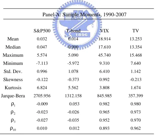
< Table 1 is inserted about here >

In Table 1, Panel A, presents univariate statistics for the data series over the period

26

indicated that T-bond is more volatile than S&P500 by the individual standard deviations. For

higher moments of the return data, each of them has negative skewness and excess kurtosis,

which reveal both shifts to the left and denial of the normal distribution assumption. It is

noted that stock and bond both exhibits fat-tail distributions. Second, after the Phillips-Perron

test is adopted to test for time series stationarity of VIX and stock turnover volume

respectively, there is no further non-stationary effect needed to be modified. The other parts

of Table 1 are the descriptive statistics of VIX and TV, where both reveals the positive means,

but the standard deviation of VIX is larger than the one of TV, appearing VIX is more volatile

than TV. As to all the data series, the Jarque-Bera statistics1largely contribute to the rejection

for the null hypothesis of a normal distribution.

As for the Panel B (Panel C) reports the sample moments over the 1990 to1997 sub-sample

(the 1998 to 2007 period). Table 1, Panel D, reports the simple unconditional correlations

between the data series over the 1990 to 2007 period. It is demonstrated that the correlation

between the stock and bond returns is negative, where is consistent to our original conjecture.

With further investigation in the change of the stock-bond correlation, we compare the two

1

The Jarque-Bera test is a goodness-of-fit measure of departure from normality, based on the sample kurtosis and skewness. The test statistic JB is defined as 2 2

( ( 3) / 4) 6

n

S + −K where S is the skewness, K is the kurtosis, and n is the number of

observations. The statistic has an asymptotic chi-squared distribution with two degrees of freedom and can be used to test the null hypothesis that the data are from a normal distribution; since samples from a normal distribution have an expected skewness of 0 and an expected kurtosis of 3.

27

sub-sample periods with each other. In Panel E, the correlation coefficients of the period

1990-1997 are shown in brackets on the upper triangle and the correlation coefficients of the

period of 1998-2007 are on the lower triangle. It is noteworthy that the unconditional

correlation between stock and bond returns in 1990-1997 is positive, while the association of

the stock and bond returns is negative in 1998-2007.

4.3 Empirical Analysis

< Table 2 is inserted about here >

In Table 2, it is documented the empirical results of the estimation with the DCCX model

over the 1990 to 2007 period. As mentioned in the Chapter III, the standard DCC model is

presented to estimate the dynamic conditional correlation between two assets. Due to the

procedure for parameters estimated under the setting of the DCC model, it is necessary to

make corresponded with the two inherent stages. In the first stage, one can utilize the GARCH

model fitted by return with individual assets for attaining standardized residuals. Furthermore,

it carries the residuals into the second stage for dynamic conditional correlation estimating.

In the Panel B of Table 2, it represents that the DCC models with different exogenous

variables. First, in the standard DCC model, the two coefficients estimated are significant

28

DCCX-a model, it is shown that the coefficient

c

₁ is negative but less significant (p-value<0.1). Alternatively, in the DCCX-b model, VIX_t−1is replaced with lagged stock turnover, the estimated coefficient

c

₂ is still negative, becoming more significant than the prior result made with DCCX-a model (p-value<0.01). Finally, the lagged VIX and lagged

stock turnover are both joint in the DCC model, named DCCX-c model, where the estimated

coefficients of the VIX and stock turnover are not only negative but highly statistically

significant (p-value<0.01). To put it more plainly, the estimated coefficients,

c

₁and

c

₂ with DCCX-c model, appear negative, which means both the lagged VIX and lagged stock

turnover negatively varied with the stock-bond returns relation. The value of Log Likelihood

Function (LLF) is reported in the Table 2, which reject the null hypothesis of the Likelihood

Ratio Test2, The more explainable variables are in the DCCX model, accompanied the larger

value of Log Likelihood Function. The increase of LLF reveals the DCCX-c model is more

explainable to the stock-bond returns correlation than the standard DCC model.

< Figure 2 is inserted about here >

As indicated in Figure 2, Panel A, This figure illustrates the substantial time-series

variation in the stock-bond returns relation over the period from 1990 to 2007. Casual

inspection of this series indicates a clustering of the periods with a negative correlation. What

has to be noticed is the change of the stock-bond returns correlation estimated by DCCX

2 2

2 ( n u ll a lte r n a tiv e) ~ ( ),

L R = − L −L χ m m is the numbers of the additional variables in the DCCX model.

29

model. Throughout the nineties until 1997/1998, we find a high positive correlation in the

neighborhood of 0.3 to 0.6, exhibiting a stable and close relationship between returns of the

S&P500 and 10-year-treasury-bonds. However, a sharp decline in the equity-bond correlation

occurred in 1997/1998, followed by a sudden reversion, then plunged back to the negative

range in 2000. Such a great decoupling of the equity-bond correlation persisted until 2007.

The correlation in the twenties fluctuates widely but mostly remains in the negative range of

-0.2 to -0.5, a stark contrast to the high positive correlation in the nineties.

Roughly speaking, we splits the sample period into 1990-1997 and 1998-2007 due to the

Asian Financial Crisis and it is demonstrated that the negative correlations are concentrated

on the periods of 1998 to 2007. These sustained negative correlation over the period of 1990,

1997-1999, and the most periods from 2000 through 2007. These observations may indicate

that the Persian Gulf War (August 1990 through February 1991), the Asian financial crisis of

the late 1997 and the Russian financial crisis of 1998 for the possible reasons particularly

influential in our results. Besides, there is an Internet Bubble crisis in 2000, which is a great

shock to the American economy, causes an overall collapse in the financial market. In 2007,

the crisis of recent sub-prime issue may be viewed as a case in point.

30

periods of high VIX or increases in VIX are associated with the periods of negative

correlations of the stock-bond returns comovement in Panel A. Figure 2, Panel C, represents

the time-series of the stock turnover. It is presented that the stock turnover flatly increases

over the sample period. However, there are more dramatically volatile when the stock-bond

correlation or the VIX also shifting enormously.

< Table 3 is inserted about here >

Table 3 represents the sub-sample data series estimated by the DCCX model from 1990 to

1997. It is shown that the VIX and the stock turnover are also negatively connected with the

stock-bond returns correlation and statistically significant.

< Table 4 is inserted about here >

The result for the second sub-period 1998-2007 in Table 4 is qualitatively similar but even

more significantly. It is denoted that the estimated coefficients of the VIX is -0.017

(p-value<0.01) and coefficient of stock turnover is -0.014 (p-value<0.01). Namely, it is found

out the inverse relationship of the equity and bond linked with the VIX and stock turnover.

< Figure 3 is inserted about here >

We depict the equity-bond correlation for the 1990-1997 sub-period in Figure 3, Panel A to

further investigate the fluctuation of stock-bond returns correlation. It is indicated more

clearly that the dynamic conditional correlation for stock and bond returns is roughly positive

31

immediately. Compared with the Panel B, the same sub-period for the VIX data series, shows

the pattern which reflect the opposite movement to the stock-bond returns correlation. In other

words, when the VIX moves up, the stock-bond returns correlation tends downward.

Additionally, the stock turnover is similar with the effects of the VIX associated with the

stock-bond returns correlation. More steeply the stock turnover moves, more volatile the

stock-bond returns relation shifts.

< Figure 4 is inserted about here >

The Figure 4 reports the similar results to the discussion above. It is more obvious to see

the inverse movement between the stock-bond returns relation and the VIX during 1998-2007

in Panel A and Panel B. The Panel C shows when the stock turnover fluctuates more

markedly, the possibility of observing the negative stock-bond returns correlation increases.

< Table 5 is inserted about here >

Table 5 reports results from estimating the following regression:

0 1 1+ 2ln( 1) 3ln(TV )t-1

t t t t

Cr =a +a Cr₋ a VIX ₋ +a +ν

Where C r_t are the dynamic conditional correlation of daily S&P500 stock and 10-year

T-bond returns. ln (V IX_t−1) is the natural log of the CBOE’s VIX at the end of period t−1, in

annualized standard deviation units. l n (T Vt−1) _{is the natural log of turnover volume of} S&P500 at the period t-1 in daily and in thousand units. C r_t−1is dynamic conditional

32

overall sample period is 1990 to 2007 The sub-period of 1990-1997 and the 1998-2007 are

also reported. The regression is estimated by OLS and T-statistics are in parentheses,

calculated with White Heteroskedasticity-Consistent Standard Errors.

The lagged VIX and the lagged stock turnover are revealed statistically significant

(p-value<0.01) and the negative association with the stock-bond returns correlation in

1990-2007 and 1998-2007. However, for the 1990-1997 sub-period, the both variables are not

significant but still negative. Accordingly, it is proved that the stock-bond returns correlation

is negatively linked with the proxies of market uncertainty-the VIX and the stock turnover.

< Figure 5 is inserted about here >

Figure 5, Panel A and Panel B compares the DCCX model with the standard DCC model in

the period 1990-2007. It is supported that the display is similar and the estimation is also

consistent.

V. Conclusion

The DCCX model advanced in this paper provides a structural form model for conditional

correlations while the standard DCC model is a reduced-form model. That is, the DCCX

model is more general to apply to the financial or economic issues. This article represents a

33

market uncertainty is associated with differences in the stock-bond returns relation. This

investigation further evaluates the empirical relevance of cross-market hedging and addresses

the notion of flight-to-quality versus flight-from-quality with increased versus decreased

stock uncertainty. It is discovered several striking results in our empirical investigation. First,

it is found a negative stock-bond returns relation with the two measures of market uncertainty,

i.e. the VIX and the stock turnover. More accurately, by means of the modified DCC model,

it is explored that stock-bond returns correlation tends to be negative (positive), during

periods when VIX increases (decreases) and during periods when unexpected stock turnover

is high (low).

In the future, we can extend the sample period including the 1980-1990 to search if the

similar phenomenon exists. Besides, to consider more other exogenous variables is also

necessary for finding out other explanation about the correlation. And the empirical study in

other countries needs more investigation to support our consequence.

34

References

Ang, A., and Chen, J., 2002, Asymmetric Correlations of Equity Portfolios, Journal of

Financial Economics 63, 443–494.

Bekaert, G., and Grenadier, S., 2001, Stock and Bond Pricing in an Affine Economy, Working Paper, Columbia University.

Black, F., 1976, Studies in Stock Price Volatility Changes, Proceedings of the 1976 Business Meeting of the Business and Economic Statistics Section, American Statistical Association, 177-181.

Bollerslev,T., 1986, Generalized Autoregressive Conditional Heteroskedasticity, Journal of

Econometrics 31, 307-327.

Bollerslev,T., Engle, R., and Wooldridge, J. M., 1988, A Capital Asset Pricing Model with Time Varying Covariances, Journal of Political Economy 96, 116-31.

Bollerslev,T., 1990, Modeling the Coherence in Short-run Nominal Exchange Rates: A Multivariate Generalized ARCH Model, Review of Economics and Statistics 72, 498-505.

Campbell, J. Y., Grossman, S. J., and Wang, J., 1994, Trading Volume and Serial Correlation in Stock Returns, Quarterly Journal of Economics 108, 905-939.

Cao, M. and Wei, J., 2007, Commonality in Liquidity: Evidence from the Option Market, Working Paper.

Chou, P. H., Chang, Y. C. and Lin, M. C., 2007, Investor Sentiment and Stock Returns in Taiwan, Review of Securities and Futures Markets19, 153-190.

Chordia, T., Sarkar, A., and Subrahmanyam, A., 2001, Common Determinants of Bond and Stock Market Liquidity: The Impact of Financial Crises, Monetary Policy, and Mutual Fund Flows, Working Paper, Emory University, the Federal Reserve Bank of New York, and UCLA.

Connolly, R., and Stivers, C., 2003, Momentum and Reversals in Equity-Index Returns During Periods of Abnormal Turnover and Return Dispersion, The Journal of Finance58, 1521-1556.

35

Connolly, R., and Stivers, C., and Sun, L., 2005, Stock Market Uncertainty and the Stock-Bond Return Relation, Journal of Financial and Quantitative Analysis40, 161-194.

David, A., and Veronesi, P., 2001, Inflation and Earnings Uncertainty and the Volatility of Asset Prices: An Empirical Investigation, Working Paper, University of Chicago.

David, A., and Veronesi, P., 2002, Option Prices with Uncertain Fundamentals: Theory and Evidence on the Dynamics of Implied Volatilities, Working Paper, University of Chicago.

Engle, R. F., 1982, Autoregressive Conditional Heteroskedasticity with Estimates of the Variance of U.K. Inflation, Econometrica 50, 987-1008.

Engle, R. F. and Sheppard, K., 2001, Theoretical and Empirical Properties of Dynamic

Conditional Correlation Multivariate GARCH, Working Paper, University of California, San Diego.

Engle, R.F., 2002, Dynamic Conditional Correlation: A Simple Class of Multivariate GARCH Models, Journal of Business and Economic Statistics 20, 339-350.

Engle, R.F., Cappiello, L., and Sheppard, K., 2006, Asymmetric Dynamics in the Correlations of Global Equity and Bond Returns, Journal of Financial Econometrics 4,537-572.

Fama, E. F. 1965, The Behavior of Stock Market Prices, Journal of Business 38, 34-105.

Fleming, J., Ostdiek, B., and Whaley, R., 1995, Predicting Stock Market Volatility: A New Measure, Journal of Futures Markets15, 265-302.

Fleming, J., Kirby, C., and Ostdiek, B., 1998, Information and Volatility Linkages in the Stock, Bond, and Money Markets.” Journal of Financial Economics 49, 111-137.

Fleming, J., Kirby, C., and Ostdiek, B., 2003, The Economic Value of Volatility Timing Using “Realized” Volatility, Journal of Financial Economics 67, 473-509.

French, K. R. and Roll R., 1986, Stock Return Variances: The Arrival of Information and the Reaction of Traders, Journal of Financial Economics 17, 99-117.

36

Glosten, L., Jagannathan, R., and Runkle, D., 1993, On the Relation between the Expected Value and the Volatility on the Nominal Excess Returns on Stocks, Journal of Finance 48, 1779-1801.

Hafner, C. M., and Franses, P. H., 2003, A Generalized Dynamic Conditional Correlation Model for Many Asset Returns, Working Paper, Erasmus University Rotterdam.

Hartmann, P., Straetmans, S., and Devries, C., 2001, Asset Market Linkages in Crisis Periods, Working Paper, European Central Bank.

Hamilton, J.,1994, Time-series Analysis, Princeton University Press, Princeton, New Jersey.

Kanas, 1998, Volatility Spillovers across Equity Markets: European Evidence, Applied

Financial Economics 8, 245.

King, M., and Wadhwani, S.,1990, Transmission of Volatility between Stock Markets, The

Review of Financial Studies 3, 5-33.

Kodres, L., and Pritsker, M., 2002, A Rational Expectations Model of Financial Contagion,

The Journal of Finance 57, 769-799.

Kroner, K. F., and Ng, V .K., 1998, Modeling Asymmetric Comovements of Asset Returns,

The Review of Financial Studies 11, 817-844.

Li, L., 2002, Correlation of Stock and Bond Returns, Working Paper, Yale University.

Liu, Y. A., and Pan, M. S., 1997, Mean and Volatility Spillover Effects in the U.S and Pacific-Basin Stock Markets, Multinational Finance Journal 1, 47-62.

Longin, L. and Solnik B., 2001, Extreme Correlation of International Equity Markets, The

Journal of Finance 56, 649-676.

Mamaysky, H., 2002, Market Prices of Risk and Return Predictability in a Joint Stock-Bond Pricing Model, Working Paper, Yale School of Management.

Mandelbrot, B., 1963, The Variation of Certain Speculative Prices, Journal of Business 36, 394-419.

37

Masih, R. and Masih, A.M.M.,1997, A Comparative Analysis of the Propagation of Stock Market Fluctuations in Alternative Models of Dynamic Causal Linkages, Applied Financial

Economics 7,59-74.

Nelson, D., 1991, Conditional Heteroskedasticity in Asset Returns: A New Approach,

Econometrica 59, 347-70.

Newey,W.K., and McFadden, D., 1994, Large Sample Estimation and Hypothesis Testing,

Handbook of Econometrics 4, Chapter 36.

Officer, R. R., 1973, The Variability of the Market Factor of New York Stock Exchange,

Journal of Business 46, 434-453.

Schwert, G. W., 1989, Why Does Stock Market Volatility Change Over Time? , Journal of

Finance 44, 1115-1153.

Tse, Y. K., and Tsui, A. K. C., 2002, A Multivariate GARCH Model with Time-varying Correlations, Journal of Business and Economic Statistics 20, 351-362.

Veronesi, P., 1999, Stock Market Overreaction to Bad News in Good Times: A Rational Expectations Equilibrium Model, The Review of Financial Studies 12, 975-1007.

Veronesi, P.,2001, Belief-dependent Utilities, Aversion to State-uncertainty and Asset Prices, Working Paper, University of Chicago.

White, H., 1994, Estimation, Inference, and Specification Analysis, Cambridge University Press.

Zakoian, J.M., 1994, Threshold Heteroskedastic Models, Journal of Economic Dynamics and