TIME AND FREQUENCY DOMAIN IDENTIFICATION AND
ANALYSIS OF A PERMANENT MAGNET SYNCHRONOUS
SERVO MOTOR
Jui-Jung Liu, Ya-Wei Lee, Fu-Cheng Wang, Ramesh Uppala, and Ping-Hei Chen*
ABSTRACT
This study employed the approach of non-linear autoregressive moving average model with exogenous inputs (NARMAX) to analyze the dynamics of a Permanent Magnet Synchronous Motor (PMSM). The non-linearity in PMSM including cogging force, reluctance force and force ripple is difficult to estimate. By using the NARMAX approach, thrust-speed relationship and thrust-position relationship could be analyzed by identifying both time and frequency domain models of the system. The frequency domain analysis is studied by mapping the discrete-time NARMAX models into gen-eralized frequency response functions (GFRFs) to reveal the non-linear coupling be-tween the various input spectral components and the energy transfer mechanisms in the system. From the results, the interpretation of the higher-order GFRFs has been comprehensively studied and non-linear effects have been related to the physical models of the systems.
Key Words: Identification; non-linear system, frequency response functions.
*Corresponding author. (Tel: 33662689; Fax: 886-2-23670781; Email: [email protected])
J. J. Liu is with the Department of Information and Electronic Commerce, Kainan University, Taoyuan 338, Taiwan
Y. W. Lee, F. C. Wang, R. Uppala, and P. H. Chen are with the Department of Mechanical Engineering, National Taiwan University, Taipei 106, Taiwan
I. INTRODUCTION
Many Permanent magnet synchronous motor (PMSM) response studies have been carried out us-ing various approaches for modellus-ing the speed and torque control system (Jahns and Soong, 1996; Solsona et al., 2000; Bolognani et al., 2001). These investigations may be classified into time domain and frequency domain methods, which involve numeri-cal integration of motions, neuro fuzzy optimization techniques and experimental estimation. These meth-ods are well suited to explain many of the non-linear dynamic behaviours associated with PMSM systems. Cheng and Tzou (2004) developed a novel design approach by applying gradient optimization with step-sizing techniques to design a digital PMSM servo drive, and the servo responses were then fed back to evaluate the overall system performances. Hattori et
al. (2001) projected a suppression control method which used repetitive control with auto-tuning func-tion and Fourier transform to the motor frame vibra-tion and the rotavibra-tional speed vibravibra-tion. Yue et al. (2003) derived a mathematical model of PMSM with initial rotor position uncertainty and proposed the control methodology. Babak et al. (2004) provided an online identification method to limit the param-eter uncertainties. This method did not need a well-known initial rotor position and made the sensorless control more robust with respect to the stator resis-tance variations at low speed. All these studies have been extensively explored, studied and documented by (Driss et al., 2001; Mobarakeh et al., 2001; Morimoto et al., 2002). Frequency domain methods are quite efficient for performing stochastic analysis. However, prior to frequency domain analysis a Fast Fourier Transform (FFT) is usually employed to trans-form the time domain signal to a spectrum distribu-tion on a linear frequency domain (Kadjoudj et al., 2001; 2003; 2004). Therefore, the dynamic charac-teristics of a nonlinear system could be shown by the power spectral density (PSD) derived from experi-mental data.
gain compression/expansion may exist simultaneously, which are generated within frequencies, and these cause nonlinear phenomena in the frequency domain. Analy-sis of non-linear systems in the frequency domain is advantageous as integral equations which relate the input-output in the time domain become algebraic in the frequency domain. In academia, non-linear sys-tem analysis and prediction to a gray or black syssys-tem have been an important issue, but many studies de-scribed non-linear systems just by a linear approach in consideration of the complicated estimation process. The present study is based on the NARMAX (Non-linear Auto-Regressive Moving Average with eXgenous inputs) (Leontaris and Billings, 1985; Bill-ings and Voon, 1986; BillBill-ings et al., 1989; Brown and Harris, 1994) modelling technique to build a model which can predict the rotor velocity and position accurately. Thereafter, by applying a recursive probing algorithm to NARMAX models, it is possible to ob-tain the non-linear frequency response functions of real systems so that the analysis and application of non-linear transfer functions become more practical. Recently, system identification has become a very active subject in research. Thouverez and Jezequel (1996) used the modal co-ordinates to ex-press the NARMAX model which reduced the num-ber of parameters to identify a mass-spring system. Liu et al. (2001) proposed a new graphical user in-terface interpretation tool for the non-linear frequency response function, and demonstrated the improved visualization of the multi-dimensional non-linear gen-eralized frequency responding functions (GFRFs). The present study is based on a combined approach of both the time and the frequency domains. It is shown that new insights into PMSM dynamics can be obtained from studying both time and frequency domain properties of the system. The non-linear GFRFs, which are generalizations of the linear fre-quency response functions, are shown to be crucial in system interpretation and modelling.
The thrust-speed and magnetic thrust-position relationships of PMSM are extensively studied in this paper. After a presentation of the NARMAX approach and frequency domain concepts, the identification and analysis results of PMSM model are presented in both time and frequency domain.
II. TIME AND FREQUENCY DOMAIN IDENTIFICATION TECHNIQUES 1. The NARMAX Approach
A wide class of discrete time multi-variable non-linear stochastic systems, can under appropriate assump-tions, be represented by the NARMAX model. For an m-output r-input system, it can be described as follows:
_y(k) = _α + F [_y(k – 1), ..., _y(k – ny), _u(k – d), ..., _u(k – d – nu), _ε(k –1), ..., _ε(k – nε)] + _ε(k) (1) where y (k) = y1(k) ym(k) , u (k) = u1(k) ur(k) , ε(k) = ε1(k) εm(k)
in which _y(k), _u(k) and _ε(k) represent the system output, input and prediction error respectively. d is the system time delay. is the degree of non-linear-ity and _α is a constant vector term to accommodate mean levels. _F[.] is a vector valued non-linear function. Taking the ith
row from Eq. (1) with differ-ent values of the maximum lag for each output, input and noise gives
yi(k) = α + Fl
i[y1(k –1), ..., y1(k – niy1), ...,
ym(k – 1), ..., ym(k – ni
ym),
ui(k – d), ..., u1(k – d – niu1), ..., ur(k – d), ...,
ur(k – d – ni ur), ε1(k – 1), ..., ε1(k – nε), ..., ε1(k – ni ε), ..., εm(k – 1), ..., εm(k – ni εm)] + _εi(k), k = 1, ..., m (2)
When m = r = 1, the model of Eq. (2) reduces to the single-input single-output (SISO) case as follows:
y(k) = α + Fl
[y(k – 1), ..., y(k – ny), u(k – d), ..., u(k – d – nu), ε(k –1), ..., ε(k – nε)] + ε(k) (3) where ε(k) is the residue at time k.
Tsang and Billings (1994) used an orthogonal estimator for the identification of NARMAX models. The orthogonal estimator is a simple and efficient al-gorithm that allows each coefficient in the model to be estimated. At the same time, it provides an indi-cation of the contribution that each term makes to the system output, using the error reduction ratio (ERR). In this study, when eliminating the dc offset, ERR can be defined as ERRi= gi2w i2(k)
Σ
k = 1 N y2(k)Σ
k = 1 N – 1N[Σ
y(k) k = 1 N ]2 ×100% (4)where gi are the coefficients and wi are the terms of an auxiliary model constructed in such a way that the terms wi are orthogonal to the data records. A for-ward-regression algorithm is employed at each step to select the term with the highest ERR, in other words, the term that contributes most to the reduc-tion of the residual variance.
The ERR value can be computed together with the parameter estimation to indicate the significance of each term, then the terms can be ranked according to their contribution to the overall mean squared pre-diction error.
2. Non-linear Systems Higher-order Frequency Response Functions Analysis and Interpretation The discrete polynomial NARMAX representa-tion of a particular system is not necessarily unique. If the model captures the system dynamics correctly, no matter in what form the discrete model is, it must present the correct linear and non-linear frequency content of the system. In other words, even though there may be a number of discrete time models to rep-resent a real system, the higher-order GFRFs corre-sponding to each of the discrete models should be unique.
Most conventional non-linear frequency domain representations have been based on the extensions of FFT routines to the Volterra model. A better approach, based on the estimation of parameters of a NARMAX model, has been proposed by Lang and Billings (2000), which is then used to generate the GFRFs. The advantage of using the polynomial NARMAX model is the reduction of the number of parameters which encode information from past out-puts and past inout-puts, and the smaller data set required for identification. The NARX model can be obtained from the NARMAX model by eliminating the error terms. ym(k) =
Σ
cp, q( 1, , p + q) 1, p + q= 1 LΣ
p = 0 m y(k – i)Π
i = 1 p ⋅Π
u(k – j) j = p + 1 p + q (5) y(k) =Σ
ym(k) m = 1 M (6) where ym(k) indicates the mthorder output signal, and
cp, q( 1, ..., p + q) donates the coefficient of product
of
Π
y(k – i) i = 1 p andΠ
u(k – j) j = p + 1 p + q .Transferring Eq. (6) to frequency domain, the frequency responding function can be found as (Thouverez and Jezequel, 1996):
[1 –
Σ
c1, 0( 1)e– j2π( f1+ + fn)1 1= 1 L ]Hn asym ( f1, , fn) =Σ
c0, n( 1, , n)e– j2π( f1 1+ + fn n) 1, n= 1 L +Σ
cp, q( 1, , p + q) 1, N= 1 LΣ
p = 1 n – qΣ
q = 1 n – 1 ⋅e– j2π(fn – q n – q + 1+ + fp + q p + q)H n – q, p( f1, , fn – q) +Σ
cp, 0( 1, , p) 1, 2= 1 L Hn, p( f1, , fn)Σ
p = 2 n (7) where H is frequency responding function. The re-gressive relation can be written asHn, pasym(⋅) =
Σ
Hiasym( f1, , fi)i = 1 n – p + 1
Hn – i, p – 1( fi + 1, , fn)e– j2π( f1, , fi) p. (8) The symmetry of an nth order frequency responding
function is defined as Hn sym ( f1, , fn) = 1n! Hn asym ( f1, , fn)
Σ
Sn (9)where Sn indicates all permutations of f
1, ..., fn in Hn(.).
The higher-order frequency responding func-tions deduced from NARX model can represent multi-dimensional characteristics and be used to investigate the dynamic behavior of a real system.
3. Model Validation
A strategy to evaluate the model correctness and validity is indispensable once the significant terms have been identified and estimation of associated pa-rameter values has been obtained. If validation shows that the model is not good, some of the design vari-ables of the estimation should be changed and the identification procedure should be repeated. Three ways of validating a model are used in this study: 1. One-step ahead prediction and model predicted
output: the one-step ahead prediction of the output is defined as
~y(k) = F [y(k – 1), ..., y(k – ny), u(k – d), ..., u(k – d – nu), ε(k – 1, θ~), ..., ε(k – nε, θ~)]
(10) where F[.] is the estimate of F[.], ~ ε(k, θ~) is the residue given by
This is a by-product of the regression process. From Eq. (10) the prediction is easily obtained by sub-tracting the prediction errors from the original data. At each step the model is effectively reset by in-serting the appropriate values into the right hand side of Eq. (10) and any error is therefore reset at each step. Consequently, even a poor model can produce reasonable one-step ahead predictions. For these reasons, the one-step ahead predictions do not often provide a good metric of model performance. The model predicted output (MPO) is defined as
~yMPO(k) =F [~y(k – 1), ..., ~y(k – ny), u(k – d), ...,
u(k – d – nu), 0, ..., 0] (12)
where the measured inputs are used to generate the model output. The zeros are present because the prediction errors will not be available when using the model to predict the output. It is an essential condition for accepting the model that the estimated model predicted outputs are in good agreement with the measured outputs.
2. Cross-validation test: estimated models are usually validated using an independent set of data called the validation data (test set). This is usually re-ferred to as cross-validation. The output from the model and the system are compared when they are run with the same input where the input data has not previously been used in the identification. The difference between the system output and MPO has to be as small as possible. The comparison be-tween the observed data and the model output usu-ally reveals much with regard to model anomalies not previously detected. Failure to pass the cross-validation test may also indicate that the system is not time-invariant.
3. Model validity test (correlation tests): The ap-proach consists of computing the auto-correlation function of the residues and the cross-correlation functions between the residues and the inputs. In order to extend to non-linear models, practical tests must be available to check the presence of non-linearity in both raw time series and residues from the fitted models. Many tests have been proposed, but using higher-order correlation functions for va-lidity of non-linear systems has been successful.
When the system is non-linear the residues should be unpredictable from all linear and non-lin-ear combinations of past inputs and outputs. This will be true if the following correlation tests are satisfied
φεε(τ) = δ(τ), φuε(τ) = 0 ∀ τ, φu2′ε(τ) = 0 ∀ τ, φu2′ε2′(τ) = 0 ∀ τ, φεεu(τ) = 0 ∀ τ ≥ 0 (13)
where φab(τ) = E[a(k – τ)b(k)], δ(τ) is the Kronecker delta, u(τ) and ε(τ) are the input and the residues sequence, respectively, and the single quote indicates that the mean has been removed.
III. ANALYSIS OF THE PMSM
Permanent Magnet Synchronous Motor (PMSM) drives have gained considerable attention among re-searchers recently because of several advantages. The high torque density, small size, inherent variable speed capability, and overall high performance of the drive with appropriate control strategy are some of the posi-tive aspects of the PMSM drive. Generally, for this kind of motor the individual phase excitations are synchronized with rotor position, which necessitates position sensing. Usually, mechanical position sensors, like resolvers or optical encoders, are em-ployed for this purpose. External position sensors, however, give position information with high resolu-tion and accuracy, but they have certain drawbacks. Position sensors with good accuracy are usually ex-pensive and they need proper mechanical mounting. They occupy space, and the cabling associated with sensors needs to be shielded in order to avoid cor-ruption due to external noise. Several methods have been published in the literature on sensor elimina-tion techniques with which the rotor informaelimina-tion is obtained electronically.
Because of high efficiency and linearity between torque and current, the PMSM has been widely used in many industrial applications. The position and speed sensors, which are normally mounted on PMSM, are desirable to eliminate from the standpoints of ma-chine size, weight, cost, and reliability.
System Description
There are two applications included in this ex-perimental design. First, under standard interference, non-linear identification methodology is adopted to construct the NARX models by using I/O signals of PMSM. These discrete non-linear models for PMSM contain the lag of inductance and uncertain electrical factors. Secondly, mapping of the NARX models into frequency domain, then multi-dimensional dynamic behavior of systems can be shown by high order GFRFs. The main framework of the experiment consists of a PMSM set, motor drive interface, power amplifier, Hall sensor and a control PC (Fig. 1). The measuring system is developed by real time control driving interface of a PMSM with visualized modules. When e control operations are executed, the feedback signals and control commands are transmitted by the interface card, through an ISA Bus, to the control PC. After computations, three-phase output voltage is
obtained. A real time control circle of PMSM is com-pleted by transmitting this output voltage to the mo-tor driving interface card by the same ISA Bus. The specifications of the test motor are shown in Table 1.
IV. TIME DOMAIN IDENTIFICATION The PMSM has a permanent magnet (PM) on the rotor and requires alternating stator currents to produce constant torque. Besides, the PMSM has si-nusoidal induced electromotive-force (the so-called back-emf) which contributes to the operating characteristics. In this study, electromagnetic thrust is regarded as input; rotor speed and position are re-garded as the output. Due to the variance of operat-ing time, environmental effects, or man-made errors, the parameters of PMSM may lead to bias. For this reason, accurate prediction can hardly be achieved. In this study, using a NARMAX approach to build a NARX model which represents a real PMAM system, the error term ε would be obtained from subtracting the predicted output ~y from the actual output.
1. Thrust-Speed NARX Model
The data are sampled at a rate of 500 Hz. The input data representing the electromagnetic thrust is given as sinusoidal waves which are fed into the
PMSM, while the output data is the rotor speed. Data points from 1001 to 2000 of I/O data are assumed for estimation set, and data points from 3001 to 4000 of I/O data are assumed for validation set. The I/O time series signals for validation set are shown in Fig. 2.
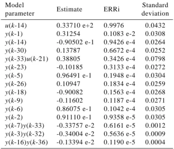
First, the power spectral density (PSD) plots of input thrust and output speed are illustrated in Fig. 3. It shows that the input and output energy occurred around the normalized frequency 0.033 but the energy mag-nitude expanded by several orders. This suggests that the system possesses non-linear dynamics around this frequency caused by electrical parameter variations. This non-linear effect would directly relate to model structures, time delays, etc. Structure selecting is im-portant to identify the non-linearity of a system. In this study, a quadratic NARX model is considered and the model structure is designed for 15 terms by rule of thumb. Setting appropriate time lags will help to de-scribe the real system and could avoid computation problems, and the appropriate maximum time lags should be set as 40 and 30 to input and output respectively for this case. It means that predicted output would be simulated by the combinations of 40 input signals and
Power amplifier 220V 60 Hz
Motor drive interface
PMSM set Hall sensor Position Speed ia , ib , ic id , iq Control computer
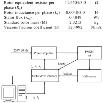
Table 1 Specification of test motor Parameter Value Unit
Rated output 83 W
Rated speed 1.0 m/sec
Rotor equivalent resistor per 11.6504/3.0 Ω phase (Rs)
Rotor inductance per phase (Ls) 0.0048/3.0 H
Stator flux (λm) 0.4849 Wb
Standard rotor mass (M) 2.3213 kg Viscous friction coefficient (B) 32.4992 N/m/s
Fig. 1 Experimental system configuration
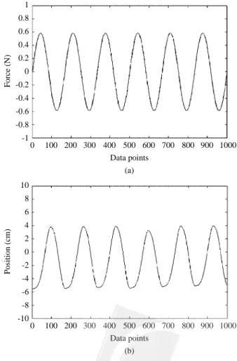
1 0.8 0.6 0.4 0.2 0 -0.2 -0.4 -0.6 -0.8 -1 0 100 200 300 400 500 Data points (a) 600 700 800 900 1000 F orce (N) 40 30 20 10 0 -10 -20 -30 -40 0 100 200 300 400 500 Data points (b) 600 700 800 900 1000 Speed (cm/sec)
Fig. 2 Input (a: thrust) and output (b: speed) of data set taken from the 1001st to 2000th samples
30 output signals. The estimation result of the I/O relationship is represented as a difference equation in Table 2. The model predicted output and cross-vali-dation tests are shown in Figs. 4 and 5 respectively where the model predicted output follows the system
output very well. It means that this time domain speed model can simulate the output speed completely and it can also play a role in speed prediction. Besides, the system is proved time-invariant. The model va-lidity tests shown in Fig. 6 indicate that the model is reasonable because the model validity tests are all in-side the confidence bands except φu2′ε2′(k) which is just
outside. It shows that this estimated model can grasp the dynamics of the PMSM precisely. This model is validated by cross validation test, correlation tests and model output prediction test, so the estimated non-linear NARX model is quite reliable to identify the relation-ship between electromagnetic torque and output speed of a PMSM.
2. Thrust-Position NARX Model
In this case, a thrust-position model is estimated 300 250 200 150 100 50 0 0 0.01 0.02 0.03 0.04 0.05 Normalized frequency f1 (a) 0.06 0.07 0.08 0.09 0.1 Magnitude 7 6 5 4 3 2 1 0 0 0.01 0.02 0.03 0.04 0.05 Normalized frequency f1 (b) 0.06 0.07 0.08 0.09 0.1 Magnitude × 105
Fig. 3 Power spectral density of (a) input signal (thrust) and (b) output signal (velocity)
40 30 20 10 0 -10 -20 -30 -40 0 100 200 300 400 500 Data points 600 700 800 900 1000 Speed (cm/sec)
Fig. 4 Comparison of the model predicted output (dotted line) with the original measurements (solid line)
Table 2 Quadratic thrust-speed NARX model
Model Standard
Estimate ERRi
parameter deviation
u(k-14) 0.33710 e+2 0.9976 0.0432
y(k-1) 0.31254 0.1083 e-2 0.0308
y(k-14) -0.90502 e-1 0.9426 e-4 0.0264
y(k-30) 0.13787 0.6672 e-4 0.0252
y(k-33)u(k-21) 0.38805 0.3426 e-4 0.0798
y(k-23) -0.10185 0.3133 e-4 0.0272
y(k-5) 0.96491 e-1 0.1948 e-4 0.0304
y(k-26) 0.10947 0.1834 e-4 0.0259
y(k-18) -0.90082 0.1563 e-4 0.0268
y(k-9) -0.11602 0.1187 e-4 0.0271
y(k-6) 0.86075 e-1 0.1042 e-4 0.0305
y(k-2) 0.91110 e-1 0.9358 e-5 0.0305
y(k-7)y(k-33) -0.33757 e-2 0.6161 e-5 0.0012
y(k-3)y(k-32) -0.34004 e-2 0.5636 e-5 0.0009
y(k-16)y(k-36) -0.13394 e-2 0.1190 e-5 0.0004
40 30 20 10 0 -10 -20 -30 -40 0 100 200 300 400 500 Data points 600 700 800 900 1000 Speed (cm/sec)
Fig. 5 Cross-validation test: original measurements (solid line) and model (asterisk line)
by the same method as above. The input is the mea-sured electromagnetic torque as sinusoidal waves and sampled at 500 Hz, and the output is the rotor posi-tion varied by the magnetic thrust. Assuming data points from 1001 to 2000 of I/O data are the data set for estimation, and data points from 3001 to 4000 of I/O data are for validation. The I/O time series sig-nals for validation set are shown in Fig. 7.
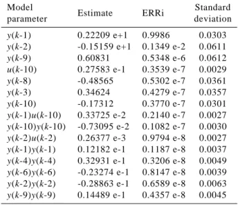
The PSD of the input thrust and output position are illustrated in Fig. 8. It shows that the input energy is around the normalized frequency 0.023 and the out-put energy frequency is around the normalized frequency 0.023 and 0. This result indicates that there exists obvious non-linearity in this system. Energy transfer occurs around a specific frequency, and this phenom-enon results in several order growth in the PSD mag-nitude from input to output signals. A quadratic NARX model is built. The maximum time lags are set as 10 to both input and output, and the estimation result of the I/O relationship is represented as a difference equa-tion listed in Table 3. The model predicted output and cross-validation test are shown in Fig. 9 and 10 respectively. The good results mean that this non-lin-ear model can describe the real system completely, and the output position can be predicted by the model. In Fig. 11, all the model validity tests satisfy the 95% confidence limit except φu2′ε2′(k) which is just outside.
It shows that this estimated model can grasp the dy-namics of the system. This model is also validated by the three tests, namely the cross validation test, the
1 0.5 0 -0.5 0 10 20 30 (e1) × (e1u1) (e1) × (e1) 40 50 0.1 0.05 0 -0.05 -0.1 0 10 20 30 (u1u1-mean) × (e1e1) 40 50 0.1 0.05 0 -0.05 -0.1 -30 -20 -10 0 10 (u1u1-mean) × (e1) (u1) × (e1) 20 30 -30 -20 -10 0 10 20 30 0.1 0.05 0 -0.05 -0.1 0.2 0.1 0 -0.1 -0.2 -30 -20 -10 0 10 20 30
Fig. 6 Model validity tests
1 0.8 0.6 0.4 0.2 0 -0.2 -0.4 -0.6 -0.8 -1 0 100 200 300 400 500 Data points (a) 600 700 800 900 1000 F orce (N) 10 8 6 4 2 0 -2 -4 -6 -8 -10 0 100 200 300 400 500 Data points (b) 600 700 800 900 1000 Position (cm)
Fig. 7 Input (a: thrust) and output (b: position) of data set taken from the 1001st to 2000th samples
correlation tests and the model output prediction test, so that the non-linear NARX model is a qualified model to identify the relationship between the thrust and po-sition of a PMSM.
V. FREQUENCY DOMAIN ANALYSIS The interpretation of non-linear effects in the frequency domain is illustrated by the higher order frequency functions computed using the models in Tables 1 and 2. The GFRFs can be directly derived from NARMAX models according to Eqs. (7) and (8). In speed NARMAX model, the first-order frequency response function H1(f) is illustrated in Fig. 12. The
resonances in H1(f) are found approximately at 0.033
in normalized frequency and the corresponding mag-nitude is 50 dB. The non-linear GFRFs are gener-ated by the non-linear terms in the discrete-time models. The second-order GFRFs H2(f1, f2) are
de-rived and represented in Fig. 13. There are four domi-nant ridges along equations f1 = 0.033, f2 = -0.033, f1
+ f2 = 0.033 and f1 + f2 = -0.033. Since the sampling
350 300 250 200 150 100 50 0 0 0.01 0.02 0.03 0.04 0.05 Normalized frequency f1 (a) 0.06 0.07 0.08 0.09 0.1 Magnitude 2.5 2 1.5 1 0.5 0 0 0.01 0.02 0.03 0.04 0.05 Normalized frequency f1 (b) 0.06 0.07 0.08 0.09 0.1 Magnitude × 104
Table 3. Quadratic thrust-position NARX model.
Model Standard
Estimate ERRi
parameter deviation
y(k-1) 0.22209 e+1 0.9986 0.0303
y(k-2) -0.15159 e+1 0.1349 e-2 0.0611
y(k-9) 0.60831 0.5348 e-6 0.0612
u(k-10) 0.27583 e-1 0.3539 e-7 0.0029
y(k-8) -0.48565 0.5302 e-7 0.0361
y(k-3) 0.34624 0.4279 e-7 0.0357
y(k-10) -0.17312 0.3770 e-7 0.0301
y(k-1)u(k-10) 0.33725 e-2 0.2140 e-7 0.0027
y(k-10)y(k-10) -0.73095 e-2 0.1082 e-7 0.0030
y(k-2)u(k-2) 0.26377 e-3 0.9794 e-8 0.0027
y(k-1)y(k-1) 0.12182 e-1 0.1187 e-8 0.0037
y(k-4)y(k-4) 0.32931 e-1 0.3206 e-8 0.0049
y(k-6)y(k-6) -0.23274 e-1 0.8147 e-8 0.0039
y(k-2)y(k-2) -0.28863 e-1 0.6589 e-8 0.0063
y(k-9)y(k-9) 0.14489 e-1 0.4357 e-8 0.0045
Fig. 8 Power spectral density of (a) input signal (thrust) and (b) output signal (position)
10 8 6 4 2 0 -2 -4 -6 -8 -10 0 100 200 300 400 500 Data points 600 700 800 900 1000 Position (cm)
Fig. 9 Comparison of the model predicted output (dotted line) with the original measurements (solid line)
10 8 6 4 2 0 -2 -4 -6 -8 -10 0 100 200 300 400 500 Data points 600 700 800 900 1000 Speed (cm/s)
Fig. 10 Cross-validation test (original measurements: solid line; model: asterisk line)
1 0.5 0 -0.5 0 10 20 30 (e1) × (e1u1) (e1) × (e1) 40 50 0.1 0.05 0 -0.05 -0.1 0 10 20 30 (u1u1-mean) × (e1e1) 40 50 0.1 0.05 0 -0.05 -0.1 -30 -20 -10 0 10 (u1u1-mean) × (e1) (u1) × (e1) 20 30 -30 -20 -10 0 10 20 30 0.1 0.05 0 -0.05 -0.1 0.2 0.1 0 -0.1 -0.2 -30 -20 -10 0 10 20 30
Fig. 11 Model validity tests.
55 50 45 40 35 30 0 0.01 0.02 0.03 0.04 0.05 Normalized frequency 0.06 0.07 0.08 0.09 0.1 Gain (dB) 200 150 100 50 0 -50 -100 -150 -200 0 0.01 0.02 0.03 0.04 0.05 Phase 0.06 0.07 0.08 0.09 0.1 Magnititude
Fig. 12 The first-order GFRFs and phase angle of thrust-speed model 0 0.05 0.1 0.15 0.2 0.25 0 -0.05 -0.1 -0.15 Normalized frequency f2 (b) (a) -0.2 -0.25 Normalized frequenc y f1 100 0 -100 H2 (dB) 0 0.05 0.1 0.15 0.2 0.25-0.25 -0.2 -0.15 -0.1 -0.05 0
Normalized frequency f1 Normalized frequency f2
Fig. 13 The second-order GFRFs of thrust-speed model: (a) top view, and (b) contour
frequency is 500 Hz, the actual frequencies are ap-proximately f1 = 16.5 Hz, f2 = -16.5 Hz, f1 + f2 = 16.5
Hz and f1 + f2 = -16.5 Hz. These functions reveal
that there appears to be a strong non-linear effect of the system which transfers energy to around 16.5 Hz as defined by the dominant ridges in 16.5 Hz. The results show that all possible frequency combinations are caused by second order non-linear effects (for example cogging torque). This can be confirmed by the power spectral density of the system output in which the power is concentrated on the normalized frequency around 0.033.
The functions f1 + f2 = 16.5 Hz and f1 + f2 =
-16.5 Hz can be seen as a resonance behavior, where energy at the input frequencies f1 and f2, which
sat-isfy f1 + f2 = 16.5 Hz, f1 + f2 = -16.5 Hz are
trans-ferred to ±16.5 Hz frequencies. In other words, short time events are transferred to long time events. In contrast, the functions f1 = 16.5 Hz and f2 = -16.5 Hz
can be seen as a release of energy phenomena, in which input frequency components close to ±16.5 Hz are amplified by the system and transferred to fre-quency components in the output other than ±16.5 Hz. The third-order transfer functions H3(f1, f2, f3)
illustrated in Fig. 14 for f1 = f3 show a similar type of
amplification. The low frequencies are amplified, particularly on the ridges of normalized frequency f1 = 0.033, f2 = -0.033, f3 = 0.033, f1 + f3 = ±0.033 and
f1 + f2 + f3 = ±0.033. The true values would be found
as defined by f1 = 16.5 Hz, f2 = -16.5 Hz, f3 = 16.5
Hz, f1 + f3 = ±16.5 HZ and f1 + f2 + f3 = ±16.5 HZ.
The interpretation of H3(f1, f2, f3) is similar to that of
H2(f1, f2) because the frequency ridges listed above
correspond to the same type of dynamic effects. The functions f1 = 16.5 Hz and f2 = -16.5 Hz can be seen
as a release of energy phenomena, and the frequency combinations f1 + f3 = ±16.5 Hz and f1 + f2 + f3 = ±16.5 Hz can be seen as a resonance behavior.
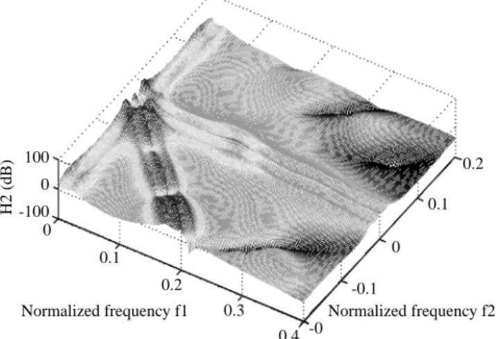
In position NARMAX model, the first-order GFRFs is illustrated in Fig. 15, including two high amplifications at 62.15 dB and 23.13 dB for low nor-malized frequencies 0 and 0.023 respectively. The sampling frequency of this case is also 500 Hz, mul-tiplied by these normalized frequency lines, and the true values would be found as defined by 0 Hz and 11.5 Hz. The magnitude of the second-order GFRFs H2(f1, f2) also shows two high magnitudes along the
normalized frequencies f1 and f2, defined by f1 = 0,
0 0.05 0.1 0.15 0.2 0.25 0 -0.05 -0.1 -0.15 Normalized frequency f2 (b) (a) -0.2 -0.25 Normalized frequenc y f1, f3 100 0 -100 H3 (dB) 0 0.05 0.1 0.15 0.2 0.25-0.25 -0.2 -0.15 -0.1 -0.05 0
Normalized frequency f1, f3 Normalized frequency f2
Fig. 14 The third-order GFRFs of thrust-speed model: (a) top view, and (b) contour 70 60 50 40 30 20 10 0 -10 0 0.01 0.02 0.03 0.04 0.05 Normalized frequency 0.06 0.07 0.08 0.09 0.1 Gain (dB) 200 150 100 50 0 -50 -100 -150 -200 0 0.01 0.02 0.03 0.04 0.05 Phase 0.06 0.07 0.08 0.09 0.1 Magnititude
Fig. 15 The first-order GFRFs and phase angle of thrust-position model
f2 = 0, f1 = 0.023, f2 = ±0.023, f1 + f2 = 0 and f1 + f2 = ±0.023 (Fig. 16). The true values would be found as defined by f1 = 0 Hz, f2 = 0 Hz, f1 = 11.5 Hz, f2 = ±11.5 Hz, f1 + f2 = 0 Hz and f1 + f2 = ±11.5 Hz.
These functions represent a strong non-linear effect as compression and expansion of energy. The functions f1 + f2 = 0 Hz and f1 + f2 = ±11.5 Hz can
be seen as resonance behaviors which represent a phenomenon of energy storage, where energy at the input frequencies f1 and f2, which satisfy f1 + f2 =
0 Hz and f1 + f2 = ±11.5 Hz, is transferred to very low
frequencies, close to 0 Hz and 11.5 Hz. The func-tions f1 = 0 Hz, f2 = 0 Hz, f1 = 11.5 Hz, f2 = ±11.5 Hz,
can be seen as a phenomenon of energy release, in which input frequency components close to 0 Hz or 11.5 Hz are amplified by the system and transferred to frequency components in the output other than these two frequencies. The low frequency compo-nents in this case correspond to long time events, which are transferred by non-linear effects to higher frequency or shorter time events.
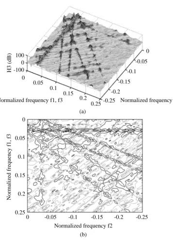
The third-order transfer function H3(f1, f2, f3)
il-lustrated in Fig. 17 for f1 = f3 shows a similar type of
amplification. The low frequencies are amplified, par-ticularly on the ridges of normalized frequencies f1 =
0, f2 = 0, f3 = 0, f1 = 0.023, f2 = ±0.023, f3 = 0.023, f1 +
f3 =0, f1 + f3 = ±0.023, f1 + f2 + f3 = 0 and f1 + f2 + f3 = ±0.023. The true values would be found as defined by f1 = 0 Hz, f2 = 0 Hz, f3 = 0 Hz, f1 = 11.5 Hz, f2 = ±11.
5 Hz, f3 = 11.5 Hz, f1 + f3 = 0 Hz, f1 + f3 = ±11.5 Hz,
f1 + f2 + f3 = 0 Hz and f1 + f2 + f3 = ±11.5 Hz.
It is important to note that even though the mod-els analyzed are different in terms of model structure, all the models generated give almost identical GFRFs. The frequency ridges are regarded as resonant peaks and they can be verified by the PSD plots. Besides, the frequency domain response functions are seen as invariants of a non-linear system.
VI. CONCLUSIONS
A combined time and frequency domain identifi-cation approach is considered in this study to analyze data from a PMSM. The NARMAX methodology has been applied to two systems. The first one utilizes the electromagnetic thrust as input and the rotor speed as output, where the second one utilizes the rotor posi-tion as output. It has been shown that this motor system, which is non-linear for the considered operating points and electromagnetic thrust, can be modeled with a se-ries of discrete-time NARMAX models, derived for various conditions and constraints.
Applying the NARMAX methodology to this type of system is proved to be a good estimation method, and the novelty of the present results relates to the non-linear frequency domain analysis by the high-order GFRFs which are derived for polynomial NARX models. The GFRFs reveal, for the PMSM application, non-linear couplings which represent energy release and storage between input harmonic components taking place at low frequency and also on particular lines of frequency. Analytical expres-sions for GFRFs for non-linear systems provide a great deal of insight into the relationship between the time and frequency domain representations of non-linear systems and can be used to study the sensitivity of the frequency domain effects due to the parameter variations in the models.
NOMENCLATURE
c coefficients of NARMAX model
d system time delay
f frequency
F non-linear function
g coefficients of an auxiliary model H frequency responding function Fig. 16 The second-order GFRFs of thrust-position model
100 0 -100 H2 (dB) 0 0.1 0.2 0.3 0.4 -0 -0.1 0 0.1 0.2
Normalized frequency f1 Normalized frequency f2
200 0 -200 H3 (dB) 0 0.1 0.2 0.3 0.4 -0.2 -0.1 0 0.1 0.2
Normalized frequency f1, f3 Normalized frequency f2
k time
m number of input
r number of output
n time lag
S all permutations of frequencies w terms of an auxiliary model
u system input
y system output
ε residue
α constant vector term
δ Kronecker delta τ time lag φ correlation tests Superscripts asym asymmetry degree of non-linearity sym symmetry Subscripts
MPO model predicted output
m number of input n order p order of input q order of output r number of output u system intput y system output ε residue REFERENCES
Babak, N. M., Farid, M. T., and Sargos, F. M., 2004, “Mechanical Sensorless Control of PMSM with Online Estimation of Stator Resistance,” IEEE Transactions on Industry Applications, Vol. 40, No. 2, pp. 457-471.
Billings, S. A., Chen, S., and Backhouse, R. J., 1989, “Identification of Linear and Non-Linear Models of a Turbocharged Automotive Diesel Engine,” Mechanical Systems Signal Process, Vol. 3, No. 2, pp. 123-142.
Billings, S. A., and Voon, W. S. F., 1986, “Correla-tion Based Model Validity Tests for Non-Linear Models,” International Journal of Control, Vol. 44, No. 1, pp. 235-244.
Bolognani, S., Zigliotto, M., and Zordan, M., 2001, “Extended-Range PMSM Sensorless Speed Drive Based on Stochastic Filtering,” IEEE Transactions on Power Electronics, Vol. 16, No. 1, pp. 110-117. Brown, M., and Harris, C., 1994, Neuro fuzzy adaptive modelling and control, Prentice-Hall, London, UK. Cheng, K. Y., and Tzou, Y. Y., 2004, “Fuzzy Opti-mization Techniques Applied to the Design of a
Digital PMSM Servo Drive,” IEEE Transactions on Power Electronics, Vol. 19, No. 4, pp. 1085-1099.
Driss, Y., Mohammed, A., and Abdallah, S., 2001, “A New Position and Speed Estimation Technique for PMSM with Drift Correction of the Flux Linkage,” Electric Power Components and Systems, Vol. 29, No. 7, pp. 597-613.
Hattori, S., Ishida, M., and Hori, T., 2001, “Vibra-tion Suppression Control Method for PMSM Utilizing Repetitive Control with Auto-Tuning Func-tion and Fourier Transform,” IEEE Annual Industrial Electronics Society Conference, Denver, USA, Vol. 1, pp. 1673-1679.
Jahns, T. M., and Soong, W. L., 1996, “Pulsating Torque Minimization Techniques for Permanent-Magnet AC Motor Drives-A Review,” IEEE Transactions on Industrial Electronics, Vol. 43, No. 2, pp. 321-330.
Kadjoudj, M., Abdessemed, R., Golea, N., and Benbouzid, M. E. H., 2001, “Adaptive Fuzzy Logic Control for High Performance PM Synchro-nous Drives,” Electric Power Components and Systems, Vol. 29, No. 9, pp. 789-807.
Kadjoudj, M., Benbouzid, M. E. H., Abdessemed, R., and Ghennai, C., 2003, “Variable Bands Hys-teresis Current Controllers for VSI-Fed PMSM Drive,” Modelling, Measurement and Control A, Vol. 76, No. 1-2, pp. 39-55.
Kadjoudj, M., Benbouzid, M. E. H., Ghennai, C., and Diallo, D., 2004, “A Robust Hybrid Current Con-trol for Permanent-Magnet Synchronous Motor Drive,” IEEE Transactions on Energy Conversion, Vol. 19, No. 1, pp. 109-115.
Lang, Z. Q., and Billings, S. A., 2000, “Evaluation of Output Frequency Responses of Nonlinear Sys-tems under Multiple Inputs,” IEEE Transactions on Circuits and Systems II: Analog and Digital Signal Processing, Vol. 47, No. 1, pp. 28-38. Leontaris, I. J., and Billings, S. A., 1985,
“Input-Out-put Parametric Models for Non-Linear Systems,” International Journal of Control, Vol. 41, No. 2, pp. 311-341.
Liu, J. J., Cheng, S. J., Kung, I. C., Chang, H. C., and Billings, S. A., 2001, “Non-Linear System Iden-tification and Fault Diagnosis Using a New GUI Interpretation Tool,” Mathematics and Comput-ers in Simulation, Vol. 54, No. 6, pp. 425-449. Mobarakeh, B. N., Meibody-Tabar, F., and Sargos,
F. M., 2001, “Robustness Study of a Model-Based Technique for Mechanical Sensorless PMSM,” IEEE Annual Power Electronics Specialists Conference, Vancouver, Canada, Vol. 2, pp. 811-816. Morimoto, S., Kawamoto, K., Sanada, M., and
Takeda, Y., 2002, “Sensorless Control Strategy for Salient-Pole PMSM Based on Extended EMF
in Rotating Reference Frame,” IEEE Transactions on Industry Applications, Vol. 38, No. 4, pp. 1054-1061.
Solsona, J., Valla, M. I., and Muravchik, C., 2000, “On Speed and Rotor Position Estimation in Per-manent-Magnet AC Drives,” IEEE Transactions on Industrial Electronics, Vol. 47, No. 5, pp. 1176-1180.
Thouverez, F., and Jezequel, L., 1996, “Identifica-tion of NARMAX Models on a Modal Base,” Journal of Sound and Vibration, Vol. 189, No. 2, pp. 193-213.
Tsang, K. M., and Billings, S. A., 1994,
‘Two-Di-mensional Pattern Analysis and Classification Using a Complex Orthogonal Estimation Algorithm,” IEE Proceedings: Vision, Image and Signal Processing, Vol. 141, No. 5, pp. 339-347.
Yue, X., Vilathgamuwa, D. M., and Tseng, K. J., 2003, “Observer-Based Robust Adaptive Control of PMSM with Initial Rotor Position Uncertainty, ” IEEE Transactions on Industry Applications, Vol. 39, No. 3, pp. 645-656.
Manuscript Received: Mar. 11, 2005 Revision Received: Aug. 15, 2005 and Accepted: Sep. 09, 2005