國 立 交 通 大 學
資訊科學與工程研究所
碩 士 論 文
貪婪演算法使用接收訊號強度指標達成室內
定位建構於群蜂無線網路
A Greedy Algorithm for RSSI-Based Indoor
Location Estimation in ZigBee wireless
Networks
研 究 生:吳佳穎
指導教授:蔡文錦 博士
貪婪演算法使用接收訊號強度指標達成室內定位建構於群蜂無線網路
A Greedy Algorithm for RSSI-Based Indoor Location Estimation in
ZigBee wireless Networks
研 究 生:吳佳穎 Student:Chia-Ying Wu
指導教授:蔡文錦 Advisor:W. J. Tsai
國 立 交 通 大 學
資訊科學與工程研究所
碩 士 論 文
A ThesisSubmitted to Institute of Computer Science and Engineering College of Computer Science
National Chiao Tung University in partial Fulfillment of the Requirements
for the Degree of Master
in
Computer Science
June 1997
Hsinchu, Taiwan, Republic of China
i
貪婪演算法使用接收訊號強度指標達成室內定位建構於群蜂無線網路
學生:吳佳穎 指導教授:蔡文錦 博士
國立交通大學資訊工程學系資訊科學與工程研究所碩士班
摘 要
越來越多的技術需要以定位技術為前提來發展, 許多商業產品、大眾
公共設施、緊急危難救助及軍事設備都有實際上的應用, 例如行車導航、
旅遊景點介紹及個人安全維護等.
在室外環境中, 全球定位系統(GPS)是最被普遍使用的, 他能夠讓使
用者知道所處的戶外地理位置, 但是全球定位系統在室內環境中會受到
建築物屏障效應的影響, 使得全球定位系統無法有效的應用在室內定位
中.
本篇論文中提出一個貪婪演算法(Greedy algorithm)使用接收訊號強
度指標達成室內定位建構於群蜂(ZigBee)無線網路, ZigBee 是一種無線網
路協定, 底層是採用 IEEE 802.15.4 標準規範的媒體存取層與實體層.
貪婪演算法會將較不準確的錨點(anchor nodes)移除, 只使用部分的錨點
去做定位, 實驗結果顯示此方法能得到更準確的定位結果.
關鍵字:室內定位、群蜂網路、訊號強度
ii
A Greedy Algorithm for RSSI-Based Indoor Location Estimation in
ZigBee wireless Networks
Student:Chia-Ying Wu Advisors:Dr. W. J.
Tsai
Institute of Computer Science and Engineering
National Chiao Tung University
ABSTRACT
In the contemporary world, the demand for positioning technologies is rising for myriad applications. Many merchandise, public transport systems, emergency rescue, and military equipment all require positioning as a foundation to functionality. Personal applications such as GPS navigation, tourist attraction descriptions, and personal safety management also show substantial demand for positioning. Commonly, Global Positioning System (GPS) is most used in an outdoor setting, allowing the user to pinpoint their geographic location. Although quite effective outdoors, the GPS is less practical in indoor location positioning due to the shielding effect that the architectural structures pose. In this thesis, the Greedy Algorithm for RSSI-Based Indoor Location Estimation in ZigBee wireless Networks is investigated. ZigBee is a specification for a suite of high level communication protocols using small, low-power digital radios based on the IEEE 802.15.4-2003standard. The Greedy algorithm waives the inaccurate anchor nodes, only using a fraction of the anchor nodes to position, resulting in more accurate and reliable positioning as shown in the Experimental Results section.
iii
誌謝
在這兩年的研究所生涯中,能完成我的碩士論文,首先最要感謝的就是我的指導 教授蔡文錦博士。在學業研究上,孜孜不倦地與我討論各種相關的議題,點出我研究 上的盲點,引導我前往正確的方向;在日常生活中,不時的關心我給予我前進的力量。 在此向我最敬愛的指導教授蔡文錦博士,致上最高的敬意。 我要感謝實驗室的學長姐,王世明、許智為、游顥榆、潘益群、黃子娟、溫善淳, 謝謝你們指導我各種研究上的相關知識。另外要感謝我的同學們,張育誠、呂威漢、 謝寧靜,謝謝你們陪伴我度過這段追求知識的過程,課業上的互相砥礪,生活中的互 相打氣,讓我從你們身上獲益良多。還有謝謝學弟,黃致遠、蕭成憲、楊巧安,謝謝 你們讓我在研究所生涯中過得更加精采,祝福你們順利畢業。 最重要的,感謝我的家人們,尤其是我的母親,在背後默默支持我,讓我在疲累 的時候有一個溫暖的避風港,謝謝你們對我有所期待及付出。 接下來要告別學生生涯,進入職場了,大家珍重。 謹以此論文獻給我的師長、家人及所有關心我的朋友們iv
CONTENTS
摘 要 ... i
ABSTRACT ...ii
Chapter 1 Introduction ... 1
1.1 Introduction to outdoor location (GPS) ... 1
1.2 Introduction to indoor location ... 2
1.2.1 Infrared ... 3
1.2.2 Ultrasonic ... 3
1.2.3 Wireless Communication ... 3
1.3 Introduction to ZigBee (IEEE 802.15.4) ... 4
Chapter 2 Related works ... 6
2.1 Four Mainstream Wireless Communication Indoor Positioning Technologies ... 6
2.1.1 Angle of Arrival (AOA) ... 6
2.1.2 Time of Arrival (TOA) ... 7
2.1.3 Time Difference of Arrival (TDOA) ... 9
2.1.4 Received Signal Strength Indicator (RSSI) ... 10
2.2 Mapping RSSI to Distance ... 11
2.3 Least Square Fitting ... 14
2.4 Mean Square Error Computation ... 15
2.5 Comparison for Existing Methods ... 17
Chapter 3 Proposed RSSI Location Algorithm ... 18
3.1 Motivation and Observation ... 18
3.2 Exhausting Method ... 20
3.2.1 Exhausting Method by Minimum MSE ... 21
3.2.2 Exhausting Method by Density ... 23
3.3 Greedy Method ... 25
v
3.3.2 Waiving rules ... 27
3.3.3 Greedy Method Flow Char ... 30
3.4 Time Complexity ... 32
Chapter 4 Experimental Results ... 34
vi
LIST OF FIGURES
Figure 2- 1 Angle of Arrival positioning based on the measurements of the
directional antenna. ... 7
Figure 2- 2 The principle of TOA using 3 Antennas radius to position. ... 8
Figure 2- 3 Time Difference of Arrival is based on the difference of distance between two points of two hyperbola and the focal point. ... 10
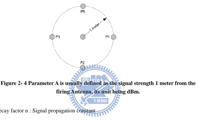
Figure 2- 4 Parameter A is usually defined as the signal strength 1 meter from the firing Antenna, its unit being dBm. ... 12
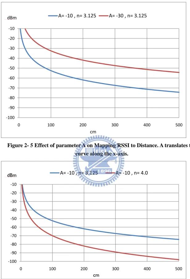
Figure 2- 5 Effect of parameter A on Mapping RSSI to Distance. A translates the curve along the x-axis. ... 13
Figure 2- 6Figure 2-6 Effect of Decay factor n on Mapping RSSI to Distance. Decay factor n affects the rate of change in curve slope. ... 13
Figure 2- 7 Calculating method of MSE. Error refers to the difference between and , is the calculated distance between the blind node coordinates and the anchor node, and refers to the distance computed from RSSI of anchor node. ... 16
Figure 3- 1 The result of mapping of RSSI to distance error from 20000 times. 19 Figure 3- 2 showing the precision of mapping of RSSI to distance error. ... 20
Figure 3- 3 The flow chart of Exhausting Method by Minimum MSE. ... 22
Figure 3- 4 The blind node locations for N subgroups, and the area with the highest density. ... 23
Figure 3- 5 The flow chart of Exhausting Method by Density. ... 24
Figure 3- 6 Waiving inaccurate anchor nodes may enhance precision of prediction. ... 26
Figure 3- 7 Waiving anchor nodes generates a negative opposite effect. ... 27
Figure 3- 8 Remove an anchor node and estimate blind node location using remaining anchor nodes in the subgroup. ... 28
Figure 3- 9 Repeat step-1 for every anchor node. ... 29
Figure 3- 10 Calculate MSE for each estimated blind node. ... 29
Figure 3- 11 Find minimum MSE and waive that not choose anchor node. ... 29
Figure 3- 12 The flow chart of Greedy Method. ... 31
Figure 4- 1 The experimental room placing 10 anchor nodes in a square orientation over 400cm*600cm. ... 34
Figure 4- 2 MEE comparison for four methods. ... 37
vii
LIST OF TABLES
Table 1 The details of IEEE 802.11b、Bluetooth and ZigBee. ... 4 Table 2 MEE comparison for existing methods. ... 17 Table 3 The experimental results, of four different method. ... 36 Table 4 The performance of Greedy method under variable number ( ) of
1
Chapter 1 Introduction
In everyday life, the questions ―where is my child,‖‖has anyone seen my keys,‖ and ―where is this place‖ are frequently asked. These questions revolve around the need for accurate positioning. As technology advances and global positioning applications mature, site location and information become readily tangible to the general public. Although very convenient, the modern city dweller spends the majority of his time indoors, which stresses the importance of indoor positioning. As such, the challenge would be to establish an indoor positioning method. The medium chosen must be convenient and technologically mature. In the case of GPS, the signals are shielded by the buildings leading to poor recognition of signal. Moreover, the GPS unit carries a high manufacturing price. Alternatively, the wireless network technology is developing rapidly, and wireless equipment may be found in most indoor settings due to its low cost. This creates an ideal platform to construct an indoor positioning environment.
1.1 Introduction to outdoor location (GPS)
The Global Positioning System (GPS) is a space-based global navigation satellite system (GNSS) that provides location and time information in all weather and at all times and anywhere on or near the Earth when and where there is an unobstructed line of sight to four or more GPS satellites. It is maintained by the United States government and is freely accessible by anyone with a GPS receiver.
A GPS receiver calculates its position by precisely timing the signals sent by GPS satellites high above the Earth. Each satellite continually transmits messages that include:
2 2. Precise orbital information (the ephemeris)
3. The general system health and rough orbits of all GPS satellites (the almanac). The receiver uses the messages it receives to determine the transit time of each message and computes the distance to each satellite. These distances along with the satellites' locations are used with the possible aid of trilateration, depending on which algorithm is used, to compute the position of the receiver. This position is then displayed, perhaps with a moving map display or latitude and longitude; elevation information may be included. Many GPS units show derived information such as direction and speed, calculated from position changes.
Three satellites might seem enough to solve for position since space has three dimensions and a position near the Earth's surface can be assumed. However, even a very small clock error multiplied by the very large speed of light — the speed at which satellite signals propagate — results in a large positional error. Therefore receivers use four or more satellites to solve for the receiver's location and time. The very accurately computed time is effectively hidden by most GPS applications, which use only the location. A few specialized GPS applications do however use the time; these include time transfer, traffic signal timing, and synchronization of cell phone base stations.
1.2 Introduction to indoor location
Generally, indoor settings are much more confined, and signal transduction is more susceptible to reflections and multi-routing due to walls. This causes confusion and deterioration of the signal. Additionally, the signal time is shorter due to a decreased path in the indoor setting, and leads to lower accuracy when positioning with the time difference method. Positioning with signal strength is also inaccurate due to low
3 fluctuations in signal in a smaller setting.
1.2.1 Infrared
Infrared[1] technologies possess the advantages of low cost and high precision, but yield to narrow angles of coverage, in turn demanding more infrared devices in a given establishment. Moreover, the infrared waves may only propagate within sight, limiting the use to a open, spacious setting, greatly limiting the potential of indoor positioning.
1.2.2 Ultrasonic
The ultrasonic[2],[3] positioning method serves as a plausible way to solve the indoor positioning problem. Being low cost and simple, ideally the ultrasonic method may deliver accurate results. The major working principle of the ultrasonic waves rely on reflective metering, or comparing the difference in propagation time of the main wave and reflected wave to accurately position. However, the ultrasonic method is influenced by multi-path and material absorption, therefore reducing range and prowess.
1.2.3 Wireless Communication
Currently, the most utilized Wireless Communication[4],[5] methods are classified as IEEE 802.11b、Bluetooth、and ZigBee(IEEE 802.15.4).
IEEE 802.11b is the most common wireless communication format, prevailing with ample bandwidth, long range, and compatibility with most systems. Nonetheless, the disadvantage is the cost of this method, demanding multiple AP as anchor nodes, and requiring power sockets for the AP units which increase the cost.
Bluetooth possesses short transmission distances and clear fall off of signal, which in turn provides accurate positioning. But these characteristics also indicate a high density of AP as anchor nodes, resulting in high power consumption and cost, rendering this method as ineffective for indoor positioning.
4
running for months or even up to a year with two AAA batteries. When constructing an indoor positioning environment, this proves advantageous because many anchor nodes may be planted at lower cost, and the transmission range of the ZigBee is very adequate for accurate positioning. The major drawback of ZigBee is deficiency in bit rate, but that may be overseen for indoor positioning demands less packets, making ZigBee ideal for this study.
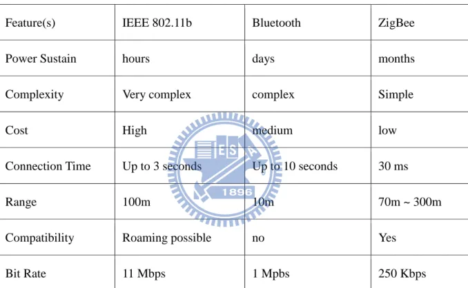
The Table 1 compares the details of IEEE 802.11b、Bluetooth and ZigBee.
Feature(s) IEEE 802.11b Bluetooth ZigBee
Power Sustain hours days months
Complexity Very complex complex Simple
Cost High medium low
Connection Time Up to 3 seconds Up to 10 seconds 30 ms
Range 100m 10m 70m ~ 300m
Compatibility Roaming possible no Yes
Bit Rate 11 Mbps 1 Mpbs 250 Kbps
Table 1 The details of IEEE 802.11b、Bluetooth and ZigBee.
1.3 Introduction to ZigBee (IEEE 802.15.4)
ZigBee[8] is a specification for a suite of high level communication protocols using small,
low-power digital radios based on the IEEE 802.15.4-2003standard.ZigBee is a low-cost,
low-power, wireless mesh networking standard. First, the low cost allows the technology to be widely deployed in wireless control and monitoring applications. Second, the low power-usage allows longer life with smaller batteries. Third, the mesh networking provides
5 high reliability and more extensive range.
The ZigBee network is ideal for text and graphic transfers. ZigBee and Bluetooth both belong to IEEE 802.15 Standard, but the ZigBee demands less power, and utilizes the 128 bit AES encryption technology, providing better security than Bluetooth.
IEEE 802.15.4-2003 Standard Characteristics:
1.This standard specifies operation in the unlicensed 2.4 GHz (worldwide),
915 MHz (Americas) and 868 MHz (Europe) ISM bands. In the 2.4 GHz band there are 16 ZigBee channels, with each channel requiring 5 MHz of bandwidth. The radios use direct-sequence spread spectrum coding, which is managed by the digital stream into the modulator. BPSK is used in the 868 and 915 MHz bands, and OQPSK that transmits four bits per symbol is used in the 2.4 GHz band. The raw, over-the-air data rate is 250 kbit/s per channel in the 2.4 GHz band, 40 kbit/s per channel in the 915 MHz band, and 20 kbit/s in the 868 MHz band. Transmission range is between 10 and 75 meters (33 and 246 feet) and up to 1500 meters for zigbee pro.
2. Low power consumption as a result of lower bit transfer rate (less data trasfer), short execution cycles and Sleep Mode.
3. Users may choose from various topology protocols such as Star, peer-to-peer, or cluster tree according to their needs.
6
Chapter 2 Related works
In this section, myriad positioning methods and the RSSI (Received Signal Strength Indication) method will be introduced, as well as Mapping RSSI to Distance, Least Square Fitting, and Mean Square Error.
2.1 Four Mainstream Wireless Communication Indoor
Positioning Technologies
Wireless Communication is generally conducted in the following four ways[6],[7]:Angle of Arrival (AOA)、Time of Arrival (TOA)、Time Difference of Arrival (TDOA)、Received Signal Strength Indicator (RSSI).
2.1.1 Angle of Arrival (AOA)
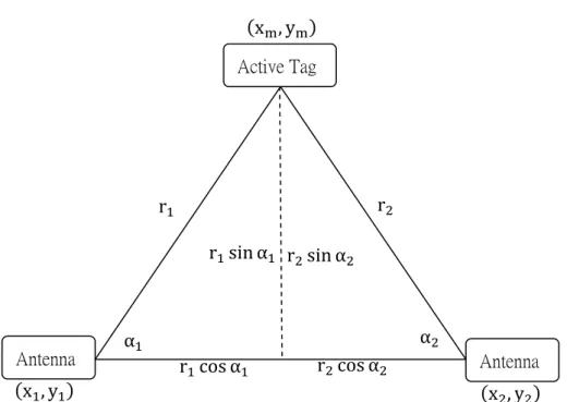
The working principle of the Angle of Arrival is based on the measurements of the Directional Antenna, obtaining the direction of the Active Tag. As shown in Figure 2-1, we may first draw a straight line originating from the antenna on a 2D plane, determine the direction of the Active Tag with two or more antennas, and pin-point the location of the Active Tag by the intersection of two lines.
As shown in the Figure 2-1, when using two Antennas to perform AOA positioning, the relationship between the Antenna and Active Tag is as follows:
(1)
(2)
( , )、( , ) and 、 are known, combining (1) and (2), we may obtain Active Tag
7
Figure 2- 1Angle of Arrival positioning based on the measurements of the directional antenna.
The advantage of AOA positioning is the lack of need to time-synchronize the Antennas; the deviations of AOA arise from the Angular Resolution of the system, or Multi-Path effect caused by barriers. The angular definition of the receiving Antenna is limited, therefore affecting positioning accuracy when the Active Tag is farther away from the Antenna. Multi-Path effect refers to the non-exclusive traverse of signal from firing Antenna to receiving Antenna, which is the main source of deviation in AOA.
2.1.2 Time of Arrival (TOA)
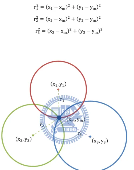
The principles of TOA are demonstrated in the figure 2-2. When using 3 Antennas to position, the distance between Active Tag and Antenna i ( i=1, 2, 3… )may be defined as:
(3) is defined as the time the fires until it reaches the Active Tag, is the time
Active Tag Antenna Antenna
8
between the signal arriving at the Active Tag, and c is the speed of light.
Using 3 radius , we may postulate the estimate of the Active
Tag by the following equation:
(4)
Figure 2- 2 The principle of TOA using 3 Antennas radius to position.
The TOA method demands precise synchronization between the Antenna and the Active Tag, thus generating working values of rt to give plausible distance estimates. Usually the Antenna possesses a deviation of a few micro-seconds, which causes errors on the calculation of distance with the TOA method. TOA may be applied to various distances,
but the fast speed of signal traverse (3 ) makes the method very sensitive to
minute time differences. Extreme precision is required in traverse time, because an error of 1 micro-second equates to a distance deviation of 300 meters, offsetting the actual position
9 of the Active Tag and the calculated position.
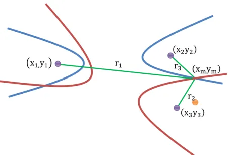
2.1.3 Time Difference of Arrival (TDOA)
TDOA, or Time Difference of Arrival is based on the difference of distance between two points of two hyperbola and the focal point. As shown in the Figure 2-3, the focal point of
the first set of hyperbola are and , the focal point of
the second set are and . The multi-Antenna TDOA
method relies on two precise readings of the time difference between two receivers, converting the information to distance, and obtaining a solution by using the simultaneous equation method on the two curves with the previously calculated results. The final solution yields the location of the Active Tag.
The distance between the Active Tag and Antenna i ( i=1, 2, 3… )may be defined as: (3)
is the time from the firing until it reaches the Active Tag, is the time taken for the signal to reach the Active Tag, c is the speed of light.
The distance between the Active Tag to Antenna j ( j=1, 2, 3… ) and Antenna k ( k=1, 2, 3… )may be defined as:
10
Figure 2- 3 Time Difference of Arrival is based on the difference of distance between two points of two hyperbola and the focal point.
Using the double hyperbola as an example, the solution of can be obtained by the
following equation:
(6)
2.1.4 Received Signal Strength Indicator (RSSI)
The RSSI Method, or Received Signal Strength Indicator Method[9],[10],[11] is based on signal strength and know channel deterioration model to estimate the distance between the reference points and subject points. The position of the subject points may be calculated with multiple distance values using similar principles as the TOA method.
In the Free Space Propagation Model, the Signal Transduction to reception power ratio is described as: (7)
11
is the signal transduction power, is the signal receiving power, is the
gain in Firing Antenna, is the gain in Receiving Antenna, (meters)is the signal
wavelength, d(meters)is the distance between Firing and Receiving ends.
Receiving signal strength is often converted to Received Signal Strength Indicator, RSSI, and its definition is:
(8)
is usually taken to be 1mW.
RSSI is Subject to Multi-Path signal decay mechanisms such as reflection、scattering、and diffraction, leading to inaccuracy of positioning.
2.2 Mapping RSSI to Distance
First, we receive the signal sent from anchor nodes (node with known coordinates, transmits wireless network signals) to blind nodes (node with unknown coordinates, determining coordinate information is the goal) as signal strength RSSI, then RSSI may be transformed to obtain a respective d value. The conversion between RSSI and d is:
(9) n: decay factor, also named signal propagation constant.
d: distance from sender.
A: received signal strength at a distance of one meter.
As seen in the equation, d is the desired distance (anchor nodes to blind node), A and n are radio signal parameters. These parameters are affected by indoor obstacles or layout, modifications of A and n may compensate for the working environment of the internet
12 apparatus.
Parameter A : RSSI value measured one meter from the sender.
As shown in the Figure 2-4, parameter A is usually defined as the signal strength 1 meter from the firing Antenna, its unit being dBm. For example, if the average received signal strength is -2dBm at 1 meter, then parameter A is -20.
Figure 2- 4 Parameter A is usually defined as the signal strength 1 meter from the firing Antenna, its unit being dBm.
Decay factor n : Signal propagation constant
Decay factor n indicates the rate of signal decay as the distance between sender and receiver increases. Larger n signifies larger rates of signal decay.
13
Figure 2- 5 Effect of parameter A on Mapping RSSI to Distance. A translates the curve along the x-axis.
Figure 2- 6Figure 2-6 Effect of Decay factor n on Mapping RSSI to Distance. Decay factor n affects the rate of change in curve slope.
-100 -90 -80 -70 -60 -50 -40 -30 -20 -10 0 100 200 300 400 500 A= -10 , n= 3.125 A= -30 , n= 3.125 ddBm cm -100 -90 -80 -70 -60 -50 -40 -30 -20 -10 0 100 200 300 400 500 A= -10 , n= 3.125 A= -10 , n= 4.0 ddBm cm
14
The above Figure 2-5 and Figure 2-6 demonstrates the effect of parameter A and Decay factor n on Mapping RSSI to Distance. parameter A translates the curve along the x-axis, Decay factor n affects the rate of change in curve slope.
2.3 Least Square Fitting
The method of least squares fitting is a standard approach to the approximate solution of overdetermined systems, i.e. sets of equations in which there are more equations than unknowns. "Least squares" means that the overall solution minimizes the sum of the squares of the errors made in solving every single equation.
The most important application is in data fitting. The best fit in the least-squares sense minimizes the sum of squared errors, an error being the difference between an observed value and the fitted value provided by a model. The sum of squared errors is used instead of the errors absolute values because this allows the errors to be treated as a continuous differentiable quantity. However, because squares of the offsets are used, outlying points can have a disproportionate effect on the fit, a property which may or may not be desirable depending on the problem at hand.
When using Least Square Fitting Positioning, n amount of anchor nodes are presented as , blind node is expressed as . The distance between the ith anchor node and blind node is expressed as , here is obtained by
RSSI conversion. and are known values, is the unknown value.
The following equations describe the relationship between anchor node coordinates、blind
node coordinates and distance :
15 Let the first n−1 equations minus the last equation
(11)
The above equations can then be written as the linear type:
(12) Where A、X and b is :
(13) (14) (15) And then, the equations can be written in the following type :
(16)
At last, the coordinates of blind node may be found from simple matrix calculations.
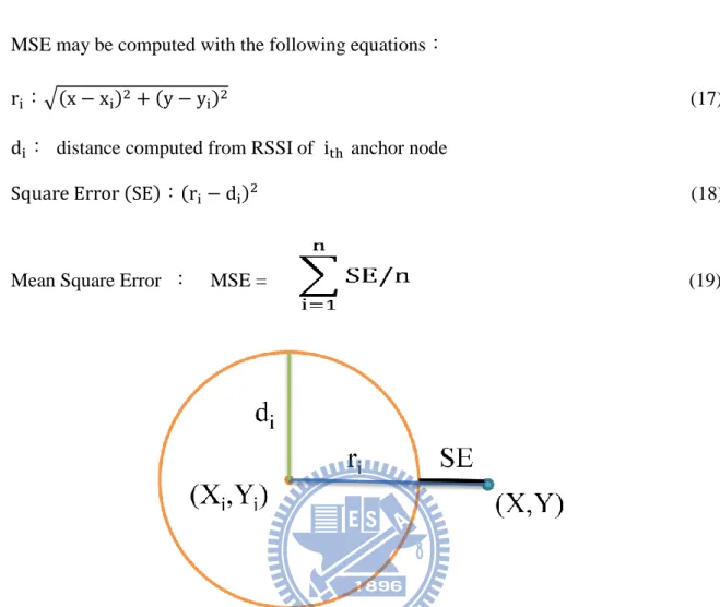
2.4 Mean Square Error Computation
MSE measures the average of the squares of the "errors." Calculating method of MSE
shows in figure 2-7. Here, error refers to the difference between and
, of which is the calculated distance
between the blind node coordinates and the anchor node, and refers to the
16
MSE may be computed with the following equations:
: (17)
: distance computed from RSSI of anchor node
: (18)
Mean Square Error : MSE = (19)
Figure 2- 7 Calculating method of MSE. Error refers to the difference between and , is the calculated distance between the blind node coordinates and the anchor node, and refers to the distance computed from RSSI of anchor node.
MSE is used specifically to assess the reliability of blind node location from RSSI information, where a lower MSE indicates a more reliable blind node location, and a higher MSE indicate the opposite. In ideal situations, or when the process of mapping RSSI to distance is entirely correct, the MSE acquired from the blind node calculated from Least Square Fitting should equal to zero. If there exists a major deviation in the mapping RSSI to distance process, a large value of MSE would be evident.
17
2.5 Comparison for Existing Methods
Table 2 is the comparison of various positioning methods that has been proposed. These methods are using RSSI and the algorithm they proposed to complete position. Types of wireless signal are IEEE 802.11 or IEEE 802.15.4, where MEE represents the mean estimation error of the method .
method Based on MEE
RSSI based WLAN Indoor Positioning with Personal Digital Assistants [12]
802.11 200cm
Use of a Simplified Maximum Likelihood Function in a WLAN-Based Location Estimation [13]
802.11 230cm
Environmental-Adaptive RSSI-Based Indoor Localization [14]
802.15.4 314cm
A New Distributed Localization Algorithm for ZigBee Wireless Networks [11]
802.15.4 197cm
Decision Experiment of Attenuation Constant During Location estimation in RSSI [10]
802.15.4 98cm
18
Chapter 3 Proposed RSSI Location Algorithm
This chapter mentions two main methods to conduct RSSI indoor location, specifically the Exhausting Method and Greedy Method. The Exhausting Method is further categorized into the method of using minimal MSE and using the highest density area to determine the final blind node coordinates.
3.1 Motivation and Observation
Current RSSI indoor positioning is still unreliable, the culprit being error generated during the mapping of RSSI to distance. There are two major causes that give rise to error. The first, radio signals fired from wireless detectors are affected by the environment, which destabilizes the signal. In this situation, two signals sent from the same distance may generate different RSSI readouts. Second, the antenna characteristics of the sensor produce variable data. The sensor may receive different RSSI values from the same distance (different direction) due to antenna receiving angle. Although this may be overcome by prior training to familiarize the antenna angles and its correlation to radio signal decay, but practically the records from training may be useless. The reason is the incapability of angle recognition between wireless sensor nodes, resulting in the acquisition of complete data which is impractical to real use.
Therefore, the biggest hurdle in RSSI indoor positioning arises from the different readouts of RSSI values from the same distance, which generates significant error during mapping RSSI to distance, ultimately influencing precision of indoor positioning.
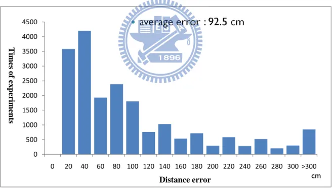
The following Figure 3-1 is the result from 20000 times, the experimental setup is in a room with 11 known node coordinates, 10 of them serve as anchor node and 1 of them acts as the blind node. Every time the blind node receives a signal from the anchor nodes, it yields the estimated distance from RSSI conversion. Comparing the estimated distance
19
with the actual distance between the anchor nodes and blind node, we may find the error value. Higher error values signify less accurate RSSI estimates.
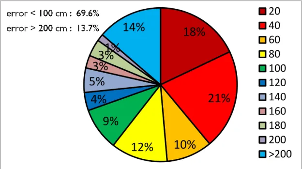
As found empirically, the figure 3-2 showing the precision of the majority of results is acceptable, with 69.6% of error within 100 cm. Albeit major consistency of error, 13.7% of error values are greater than 200cm, which severely affects the precision of indoor positioning.
Therefore, in this study, we propose to waive the comparatively inaccurate anchor node information, only using the more precise anchor node information to position, ensuring more accurate results. The major problem is to successfully identify the precision of anchor nodes.
Figure 3- 1 The result of mapping of RSSI to distance error from 20000 times.
0 500 1000 1500 2000 2500 3000 3500 4000 4500 0 20 40 60 80 100 120 140 160 180 200 220 240 260 280 300 >300 T im es of ex peri m ent s cm Distance error
20
Figure 3- 2 showing the precision of mapping of RSSI to distance error.
3.2 Exhausting Method
The method of least squares is a standard approach to the approximate solution of overdetermined systems. That is, if we obtain more than 3 RSSI values from anchor nodes, we may use least squares fitting to calculate blind node coordinates.
In an ordinary setting, more than 3 anchor nodes are usually set up, therefore during least squares fitting, not all of the anchor nodes are adopted, rather only selective anchor nodes are chosen. In other words, the anchor nodes are divided, forming many subgroups, where each subgroup contains 3 or more anchor nodes, enabling each subgroup to generate a set of blind node coordinates. The set of blind note coordinates may allow us to determine the final blind node coordinates.
Exhausting method seeks for all the subgroups, then calculates the respective blind node coordinates from the subgroups. Here we use the combination method to explore all the possible subgroups.
Given n anchor nodes, there are N subgroups, where N is :
18%
21%
10%
12%
9%
4%
5%
3%
3%
1%
14%
20
40
60
80
100
120
140
160
180
200
>200
21
From the combination method we may find all the possible subgroups, and further calculate the respective blind node coordinate from each subgroup. A mass of blind node coordinates will be obtained, and the key to the Exhausting Method is finding the final blind node coordinate from the sea of unprocessed blind node coordinates. Two strategies are proposed; one is base on minimum MSE, the other is density.
3.2.1 Exhausting Method by Minimum MSE
Exhausting method by minimum MSE is the way to determine the final blind node coordination. Specifically, among N calculated locations, choosing the one with minimum MSE is desired.
First, we divide n number of anchor nodes into N number of subgroups using the
combination method, determine the corresponding blind node locations for
from the N subgroups, Calculate N MSE say M i for 1 i N , each for
one estimated location Li x y , then among the N Li x y , the one associated with minimal MSE will be the blind node location. The Flow Chart is shown in figure 3-3:
22
Figure 3- 3 The flow chart of Exhausting Method by Minimum MSE.
Exhausting method by minimum MSE is not the most ideal method, because there is a large chance it will position mistakenly at a far away coordinate.. Errors are prone to happen during mapping RSSI to distance. For example, if one subgroup by chance generates the lowest MSE from the least square fitting blind node coordinates, this method will declare that position as the final blind node coordinate. As there exists an abundance of subgroups, the chances of the above happening increase, leading to inaccurate positioning.
23
3.2.2 Exhausting Method by Density
In lieu of the defective blind node coordinate determination by MSE of each subgroup, the exhausting method by density is considered for more accurate results. Exhausting Method by Density utilizes the Exhausting Method with multiple subgroups to calculate the corresponding blind node coordinates, then finding the most dense blind node coordinate zone, lastly averaging the coordinates in this zone to obtain the final blind node coordinates.
In Figure 3-5, first we divide all n number of anchor nodes into N number of subgroups using the combination method, calculate the blind node locations Li x y for 1 i N for the N subgroups, then locate the area(in this paper, the area is set to 20cm*20cm) with the highest density as shown in the figure 3-4. Finally, averaging all the blind node coordinates in this area will produce the final blind node location.
Figure 3- 4 The blind node locations for N subgroups, and the area with the highest density.
True blind node coordinate 20cm*20cm
24
Figure 3- 5 The flow chart of Exhausting Method by Density.
The precision of the Exhausting Method by Density is acceptable with the error in a decent margin, but the Exhausting Method is overly complicated in computation, putting stress on the positioning system, causing failure of real-time calculation of the current position.
25
3.3 Greedy Method
RSSI contains a fundamental flaw, which is unreliable RSSI-to-distance mapping. Using least square fitting directly to calculate blind node location will generate location errors far larger than the RSSI-to-distance mapping error, because the best fit in the least-squares sense minimizes the sum of squared errors instead of the errors absolute values. However, because squares of the errors are used, outlying points can have a disproportionate effect on the fit. That is, large values of RSSI-to-distance mapping error, albeit a minority in the data, pose significant effects to the data.
Although the Exhausting Method by Density only uses selected anchor nodes, but the ―highest density‖ method to estimate a blind node coordinate is not immune to incorrect anchor node information, resulting in a marginally lower error average in RSSI-to-distance mapping.
Therefore, we propose the Greedy Method, striving to waive the inaccurate anchor nodes, only using the anchor nodes with smaller RSSI-to-distance mapping error to position.
3.3.1 Effect of waiving inaccurate anchor nodes
Under normal working circumstances, waive inaccurate anchor nodes may enhance precision of prediction. In the figure 3-6 as an example, only using accurate anchor node 1、 anchor node 2 and anchor node 3 may give a dependable position xm ym . If an inaccurate anchor node 4 is inserted, the result is affected and will predict the position xn yn . If we may identify anchor node 4 as inaccurate, waive it to ensure only accurate anchor nodes are used, we may deliver more precise predictions.
26
Figure 3- 6 Waiving inaccurate anchor nodes may enhance precision of prediction.
Supposively, waiving more anchor nodes until only the least amount of anchor nodes are present (3 in this study) will give the best results. Practically, each anchor node possesses a different RSSI-to-distance mapping error, and when all anchor nodes have comparable error, waive anchor nodes may generate a negative opposite effect. In the Figure 3-7 as an example, the fine-line circle represents the actual distance, while the bold-line circle represents the RSSI-to-distance mapping distance. The intersection of the fine-line circles will be the actual position of the blind node, where x is the position determined by all four anchor nodes, y is the position after waiving anchor node 4, and z is the position after waiving anchor node 2. We may observe from the figure that x is closest to the actual position, demonstrating the undesired deviation from norm by the waiving method.
27
Figure 3- 7 Waiving anchor nodes generates a negative opposite effect.
3.3.2 Waiving rules
Moderately waiving inaccurate anchor nodes may increase precision, therefore it is crucial to isolate the anchor nodes subject to waiving. Here, we propose to find a most ―inappropriate‖ anchor node in each round and waive it. Determination of appropriateness of anchor nodes is based on the value of MSE. If waiving a certain anchor node may decrease the MSE to the lowest among other anchor nodes, then the waived anchor node would be presented as inappropriate.
There are four steps to waiving an anchor node:
Step-1: Remove an anchor node and calculate possible blind node location using
remaining anchor nodes in the subgroup.
28
Step-2 : Do step-1 for every anchor nodes. Imitating step 1, calculate the other possible
blind node location.
Step-3 : Calculate MSEs for all possible blind nodes.
Step-4 : Find minimum MSE and waive that not choose anchor node.
Figure 3-8~3-11 show the example of the four steps of waiving an anchor node. Figure 3-8 shows step 1 which waive the lower left hand corner anchor node, using only the remaining four anchor nodes to calculate the possible blind node location(dark blue sphere). Figure 3-9 shows the result of step 2, where the blind node locations after waiving each anchor node had been presented. Figure 3-10 shows the result of step 3, where the MSE of each estimation location had been calculated. Figure 3-11 shows the result that lower left hand corner anchor node will be waived because it will result in minimum MSE.
Figure 3- 8 Remove an anchor node and estimate blind node location using remaining anchor nodes in the subgroup.
29
Figure 3- 9 Repeat step-1 for every anchor node.
Figure 3- 10 Calculate MSE for each estimated blind node.
Figure 3- 11 Find minimum MSE and waive that not choose anchor node.
The point with minimum MSE
MSE=32.7
MSE=39.4 MSE=46.3 MSE=53.7 MSE=61.2
30
3.3.3 Greedy Method Flow Char
Greedy Method flow char is showing in Figure 3-12. During the Greedy method, one anchor node is waived according to the waive rule in each round. For example, if we started with k number of anchor nodes, there will be k-1 anchor nodes remaining after one round, and continue until the number of anchor nodes equals to the minimum number of reference nodes . equals to 3, because at least 3 anchor nodes are needed to calculate blind node coordinate using least square fitting. The reason to establish a minimum number of reference node is mentioned in 3.3.1. If a minimal amount of anchor nodes are used to position, blind node locations with large deviances but with marginal MSE are possible, therefore it is important to set the parameter according to different environments. When waiving anchor nodes, each possible blind node location is assessed for MSE, and the Greedy method will record all the possible blind node coordinates and their respective MSE, leading to the final blind node coordinates as characterized with the smallest MSE. The following is a flow chart of the process. n represents the total number of anchor nodes,
Lki x y represents possible blind node location, k represents the number of anchor nodes
not yet waived, i represents the anchor node in the remaining not-waived k
31
32
3.4 Time Complexity
Because the Exhausting method lists all the possible combinations of anchor nodes, it possess the problem of time complexity. Alternatively, the Greedy method evades this flaw. We may use least square fitting and square error calculation counts to compare the time complexity of these two methods.
Number of calculations need for least square fitting of:Greedy method
i n
i
Number of calculations need for least square fitting of Exhausting method:
n i n
i
If and we have a total of 10 anchor nodes, or if n 1 , the Greedy method will
need to compute 52 times of least square fitting, while the Exhausting method will need to compute 968 times of least square fitting.
Number of calculations need for square error for Greedy method:
n2
n
i
Number of calculations need for square error for Exhausting method:
n i n
i
If and we have a total of 10 anchor nodes, or if n 1 , the Greedy method will
need to calculate square error 380 times, while the Exhausting method will need to calculate the square error more than 6000 times.
33
From the hypothetical n 1 example we may notice the difference in time complexity,
where the Greedy method demonstrated the need of significantly less calculations than that of the Exhausting method.
34
Chapter 4 Experimental Results
The experimental setup is in a conference room showing in Figure 4-1, placing 10 anchor nodes in a square orientation over 400cm*600cm. Each anchor node is placed 200cm apart, and experimented on 15 different locations with 100cm gaps. Each position undergoes 100
positioning tests with mapping RSSI to distance parameter 1 , decay factor
n 3 125 , and number of minimum reference node 4 . A schematic of the
experimental setup is shown below, noting that the blind nodes are tested individually, not 15 at a time:
Figure 4- 1 The experimental room placing 10 anchor nodes in a square orientation over 400cm*600cm.
The table 3 presents the results, where mean estimation error(MEE) represents the average distance variation between the estimation blind node location and the true blind node location, its units are centimeters, and smaller MEE values indicating more precise
0 100 200 300 400 500 600 0 100 200 300 400
Blind Nodes
Anchor Nodes
35
estimates. The smaller the coefficient of variation(CV), the less deviation from the norm in the final blind node location is detected, and higher reliability is implied. In the Table 3, ‖1 -1 ‖represents the result on the coordinates (1 , 1 ), ‖ verage‖ represents the average result of the 15 different tested locations, and differences between methods may be quickly identified in this row.
As shown in the results, the Greedy method demonstrates the most accurate positionings. Viewing each point individually, only the points (100, 200) and (200, 500) have MEE lower than Exhausting method by density, the rest are all better than the other three methods. Also, except for the position (300, 200), the MEE values are all lower than 100 centimeters, with an astonishing Average of MEE of 50 centimeters, displaying very high precision. The Exhausting method by density is second to best and the Exhausting method by MSE the worst, indicating that the Exhausting method by density is more suitable for the determination of the final blind node location.
Relying on MEE to judge the functionality of a method may not be the most subjective, allowing occasional misleads but with overall low estimation error. Therefore, we must evaluate the consistency of methods by the coefficient of variation. Smaller coefficient of variation demonstrates the proximity of blind node location, and the Greedy method prevails still from the four methods. It is accurate and consistent, while the Exhausting method by density displays a high CV despite good accuracy. This notifies that the Exhausting method by density will produce results that are far from the actual blind nodes. Similarly, the least square fitting has a low CV value, but the accuracy is also low, leading to comparable results as the Exhausting method by density. In short, the coefficient of variation may facilitate in the determination of functionality between methods, but the deciding factor remains the mean estimation error.
36
Greedy method Exhausting
(density) E Exxhhaauussttiinngg ( (mmiinnMMSSEE)) Least square fitting Blind node location
MEE CV MEE CV MEE CV MEE CV
100-100 70.19 0.4213 177.38 0.215 99.17 0.565 230.54 0.179 100-200 66.38 0.083 47.2 0.247 153.89 0.321 223.81 0.293 100-300 28.35 0.129 52.69 0.268 72.69 1.219 51.22 0.108 100-400 27.43 0.538 27.79 0.51 338.4 0.305 339.25 0.212 100-500 22.8 0.181 41.34 0.296 63.62 1.736 189.16 0.165 200-100 64.74 0.286 119.43 0.664 244.93 0.437 346.34 0.075 200-200 31.83 0.543 59.86 0.663 206.28 0.475 112.32 0.199 200-300 36.75 0.22 108.23 0.453 330.46 0.179 514.67 0.104 200-400 53.857 0.126 69.03 0.346 315.12 0.296 141.3 0.163 200-500 80.74 0.146 58.1 0.445 295.72 0.443 134.71 0.097 300-100 54.77 0.133 66.63 0.367 143.86 0.247 187.7 0.13 300-200 119.38 0.029 160.34 0.132 256.63 0.196 160.78 0.032 300-300 27.9 0.33 56.89 0.398 67.86 1.568 52.69 0.297 300-400 61.64 0.158 112.99 0.394 282.55 0.252 113.04 0.171 300-500 9.78 0.713 66.01 0.69 496.49 0.182 102.81 0.041 Average 50.436 0.2691 81.594 0.4059 224.51 0.5614 193.36 0.1511
37
From the Figure 4-2, the superiority in precision of the Greedy Method is readily demonstrated.
Figure 4- 2 MEE comparison for four methods.
The Table 4 and Figure 4-3 demonstrates that under variable number of minimum reference node , the Greedy method generates different estimation precisions. As is smaller, the precision of the estimates is better. It is worth noting, though, that when
3, the average MEE is higher than when 4, showing that using the least amount of anchor nodes to position may give small MSE, but possess larger estimation error on blind node location. 0 100 200 300 400 500 Greedy method Exhausting (density) Exhausting (min MSE) Least square fitting cm
MEE
38
Number of Min Reference Nodes
Blind node location 3 4 5 6 7 8 9 10 100-100 105.14 70.19 92.28 98.34 117.2 124.04 127.14 230.54 100-200 83.51 66.38 64.98 60.87 57.9 61.95 64.28 223.81 100-300 31.64 28.35 33.95 60.87 34.53 46.8 36.46 51.22 100-400 49.23 27.43 41.67 37.77 42.96 70.63 125.56 339.25 100-500 26.77 22.8 30.93 31.98 34.6 38.61 25.26 189.16 200-100 65.48 64.74 83.05 81.52 94.54 177.42 200.17 346.34 200-200 52.85 31.83 43.44 50.71 64.03 45 205.63 112.32 200-300 35.33 36.75 36.33 37.24 114.92 108.74 183.96 514.67 200-400 58.83 53.85 56.41 65.56 70.3 48.14 88.25 141.3 200-500 91.45 80.74 94.22 70.82 69.56 40.12 109.37 134.71 300-100 62.71 54.77 48.98 47.65 54.02 67.97 108.72 187.7 300-200 119.99 119.38 119.49 112.69 124.26 160.34 163.96 160.78 300-300 37.62 27.9 35.36 30.14 32.1 36.5 28.17 52.69 300-400 83.63 61.64 87.57 89.53 80.2 117.05 121.22 113.04 300-500 22.96 9.78 21.79 22.51 29.15 53.07 82.89 102.81 Average MEE 61.80 50.43 59.36 59.88 68.01 79.75 111.4 193.36 Table 4 The performance of Greedy method under variable number ( ) of minimum
39
Figure 4- 3 MEE of Greedy method under different .
0 20 40 60 80 100 120 140 160 180 200 3 4 5 6 7 8 9 10
MEE
cm40
Chapter 5 Conclusion
In this study, two indoor RSSI positioning algorithms were proposed, each precise to within 100 centimeters. The Exhausting method uses a majority rule method, ruling out the extreme data, in turn isolating the most possible region of the blind node, successfully reducing the observed average error from 200cm of least square fitting to 100cm. The drawback of this method is the complexity of calculations to obtain results, preventing instant positioning. Alternatively, the Greedy method waives anchor nodes, screens for effective data, and successfully reduces the error produced during mapping RSSI to distance, which lowers the average error within 50 centimeters. The positioning accuracy is very high, while exempt from the overly complex calculations as seen with the Exhausting Method.
41
Reference
[1] R. Want, . Hopper, V. Falcao, and J. Gibbons, ―The ctive Badge Location ystem,‖ ACM Trans. Information Systems, pp.91-102, Jan. 1992.
[2] A. Harter, A. Hopper, P. Steggles, A. Ward, and P. Webster, ―The Anatomy of a Context- ware pplication,‖ Proc. 5th nn. Int’l Conf. Mobile Computing and Networking (Mobicom 99), ACM Press, New York, pp. 59-68, 1999.
[3] N.B. Priyantha, . hakraborty, and H. Balakrishnan, ―The Cricket
Location-Support System,‖ Proc. 6th nn. Int’l onf. Mobile Computing and Networking (Mobicom00), ACM Press, New York, pp. 32-43, 2000.
[4] I. Oppermann, L. Stoica, A. Rabbachin, Z. Shelby, and J. Haapola, ―UWB wireless sensor networks: UWEN- practical examples,‖ IEEE Commun. Mag., vol. 42, pp. S27–S32, 2004.
[5] K. Yu, J. P. Montillet, and . Rabbachin, ―UWB location and tracking for wireless embedded networks,‖ Signal Process., vol. 86, pp. 2153–2171, 2006. [6] P. Prasithsangaree, P. Krishnamurthy and P. K. hrysanthis, ―On Indoor
Position Location with Wireless LANs,‖ Proceedings of the 13th IEEE International Symposium on Personal, Indoor and Mobile Radio Communications, Vol. 2, pp. 720 -724, 2002.
[7] M. O. unay and J. Jekin, ―Mobile Location Tracking in D DM Networks Using Forward Link Time Difference of Arrival and Its Application to
Zone-Based Billing‖, Bell Labs, Lucent Technologies, 2 1.
[8] Zigbee Alliance, Zigbee-2006 specification, Available: http://www.zigbee.org/, 2006.
[9] N. Patwari, A.O. Hero, M. III, Perkins, N.S. Correal, R.J. O’Dea, ―Relative Location stimation in Wireless ensor Networks‖, IEEE Trans. Signal Processing, vol. 51, no. 8, pp. 2137-2148, 2003.
[10] K. Tateishi, T. Ikegami, ―Decision xperiment of ttenuation onstant During
42
[11] J. Chen, X.J. Wu, P.Z. Wen, F. Ye, J.W. Liu, ― New Distributed Localization lgorithm for ZigBee Wireless Networks,‖ I D , pp. 4451-4456, 2009. [12] U. Grossmann, M. Schauch, S. Hakobyan, ―RSSI based WLAN Indoor
Positioning with Personal Digital ssistants,‖ I ID 2 7 4th, pp. 653-656, 2007.
[13] S. Hara, D. nzai, ―Use of a Simplified Maximum Likelihood Function in a WLAN-Based Location stimation,‖ IEEE WCNC, pp. 1-6, 2009.
[14] Hyo- ung hn, Wonpil Yu, ‖ Environmental-Adaptive RSSI-Based Indoor Localization, ‖ IEEE Transactions on Automation Science and Engineering, vol. 6, no. 4, pp. 626-633, 2009.
[15] S. Hara, Z. Dapeng, K. Yana, j. gihara, j. Taketsugu, K. Fukui, S. Fukunaga, k. Kitayama, ―Propagation Characteristics of IEEE 802.15.4 Radio Signal and Their Application for Location Estimation,‖ IEEE VTC 2005-spring, vol. 1, pp. 97-101, 2005.
[16] J. Zhao, Y. Zhang, M. Ye, ―Research on the Received Signal Strength
Indication Location Algorithm for RFID System,‖ IEEE ISCIT, pp. 881-885, 2006.