酵素分類的預測

國

立

交

通

大

學

生物資訊所

碩

士

論

文

酵素分類的預測

Prediction of Enzyme Class

研 究 生：張世瑜

指導教授：黃鎮剛 教授

酵素分類的預測

Prediction of Enzyme Class

研 究 生：張世瑜 Student：Shih-Yu Chang

指導教授：黃鎮剛 Advisor：Jenn-Kang Hwang

國 立 交 通 大 學

生 物 資 訊 所

碩 士 論 文

Submitted to Institute of Bioinformatics College of Biological Science and Technology

National Chiao Tung University in partial Fulfillment of the Requirements

for the Degree of Master

in

Bioinformatics July 2006

Hsinchu, Taiwan, Republic of China

酵素分類的預測

學生：張世瑜 指導教授： 黃鎮剛

Prediction of Enzyme Class

student：Shih-Yu Chang Advisor：Dr. Jenn-Kang Hwang

Institute of

National Chiao Tung University

ABSTRACT

Enzymes, as a subclass of catalysts, can be separated into six parts since they have different chemical reactions and protein functions. Methods for predicting protein function from structure are becoming more important than experimental knowledge. In this study, we describe some coding schemes which include both sequence-based and structure-based protein information. We predict the enzyme class for different coding schemes with 2 methods; one is the 2-level SVM model method, one is the Huffman tree model method which is described in this study. This Huffman tree model using support vector machine (SVM) is provided to predict the enzyme classification from the unknown- function enzymes. By comparing with these methods, Huffman tree model is demonstrated useful on enzyme class predicting since we can obtain unbiased and the best prediction accuracy of 36% using the Huffman tree model.

誌謝 在研究所的兩年時間，我學到了很多，不管是課業方面，還是待人接物方面，更重 要的是一個人的態度．在做研究的時候就應該極力鑽研，秉持打破沙鍋問到底的原則， 將事物作透徹的分析；在休閒的時候，就要懂得適當地放鬆心情，不要一心二用，反而 無法兩者兼顧． 多謝我的指導老師黃鎮剛老師，老師並不光是指派任務讓我們完成，而是讓我們在 這個任務當中得到一些新的啟發，再經由這些啟發給予適當的建議，適當地指引方向． 也由於老師的教導方式，讓我知道思考在研究當中是最重要的一環． 另外還要感謝實驗室的所有同伴，在我有困難的時候給了我很多的幫助，讓我知道 了許多問題都發生在之前沒有想到會成為問題的地方．謝謝陸志豪學長不僅在研究上提 攜我，還找我一起打球運動．謝謝游景盛學長在一開始就先教我ＳＶＭ的使用，還在我 有問題的時候給我很多協助．謝謝簡思樸，盧慧及葉書瑋同學在這兩年內彼此鼓勵，互 相學習，還有最後的時候互相盯對方的進度．另外也多謝其他實驗室的學長姐們．

CONTENTS 摘要 i Abstract ii 誌謝 iii Contents iv Introduction 1 Dataset 4 Methods 4

Input coding schemes 4

Support vector machines 8

2-level support vector machine model 11

Huffman tree model 11

Results 13 Discussion 14 References 17 Tables 19 Figure captions 32 Figures 33 Appendix 50

INTRODUCTION

Catalysts, generally speaking, are specific in nature as to the type of reaction they can catalyze. Enzymes, as a subclass of catalysts, are very specific in

nature. Each enzyme can act to catalyze only very select chemical reactions and only with very select substances. An enzyme has been described as a "key" which can "unlock" complex compounds. An enzyme, as the key, must have a certain

structure or multi-dimensional shape that matches a specific section of the "substrate" (a substrate is the compound or substance which undergoes the change). Once these two components come together, certain chemical bonds within the substrate molecule change much as a lock is released, and just like the key in this illustration, the

enzyme is free to execute its duty once again.

The Enzyme Commission number (EC number) is a numerical classification scheme for enzymes, based on the chemical reactions they catalyze. As a system of enzyme nomenclature, every EC number is associated with a recommended name for the respective enzyme.

Every enzyme code consists of the letters "EC" followed by four numbers

separated by periods. Those numbers represent a progressively finer classification of the enzyme. For example, the enzyme tripeptide aminopeptidase has the code "EC 3.4.11.4", whose components indicate the following groups of enzymes: EC 3

enzymes are hydrolases (enzymes that use water to break up some other molecule), EC 3.4 are hydrolases that act on peptide bonds, EC 3.4.11 enzymes are only those hydrolases that cleave off the amino-terminal amino acid from a polypeptide, and EC 3.4.11.4 are those that cleave off the amino-terminal end from a tripeptide.

Strictly speaking, EC numbers do not specify enzymes, but enzyme-catalyzed reactions. If different enzymes (for instance from different organisms) catalyze the

same reaction, then they receive the same EC number. UniProt identifiers uniquely specify a protein by its amino acid sequence. Here are some brief introduction of six classes of enzymes in Appendix.

The enzyme nomenclature scheme was developed starting in 1955, when the International Congress of Biochemistry in Brussels set up an Enzyme Commission. The first version was published in 1961. The current sixth edition, published by the International Union of Biochemistry and Molecular Biology in 1992, contains 3196 different enzymes.

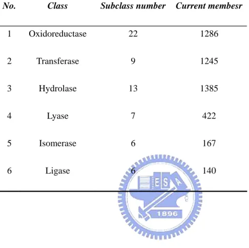
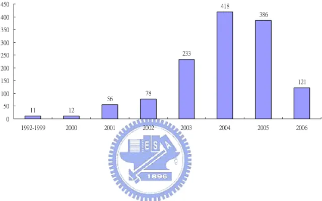
Here are some related numbers such as the number of each enzyme class or the number of subclass in each enzyme class listed in Table 1. There are more and more unknown function proteins found in recent years (see Figure 1). To know the

classification of these enzymes is important; we can know what reactions they will do, what kinds of catalytic sites they are, etc. However, enzymes are classified into six classes by experimental supports so far and it takes a lot of time. If an enzyme can be classified in computational way, it is faster, cheaper, and simpler to recognize the enzyme class in the future.

Simulating the molecular and atomic mechanisms that define the function of a protein is beyond the current knowledge of biochemistry and the capacity of available computational power. Similarity search among proteins with known function is

consequently the basis of current function prediction (Whisstock and Lesk 2003). A newly discovered protein is predicted to exert the same function as the most similar proteins in a database of known proteins. This similarity among proteins can be defined in a multitude of ways: two proteins can be regarded to be similar, if their sequences align well [e.g. PSI-BLAST (Altschul, Madden et al. 1997)], if their structures match well [e.g. DALI (Holm and Sander 1996)], if both have common

surface clefts or bindings sites [e.g. CASTp (Binkowski, Naghibzadeh et al. 2003)], similar chemical features or common interaction partners [e.g. DIP (Xenarios, Salwinski et al. 2002)], or if both contain certain motifs of amino acids (AAs) [e.g. Evolutionary Trace (Yao, Kristensen et al. 2003)]. An armada of protein function prediction systems that measure protein similarity by one of the conditions above has been developed. Each of these conditions is based on a biological hypothesis; e.g. structural similarity implies that two proteins could share a common ancestor and that they both could perform the same function as this common ancestor (Bartlett et al., 2003).

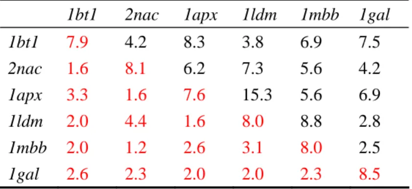
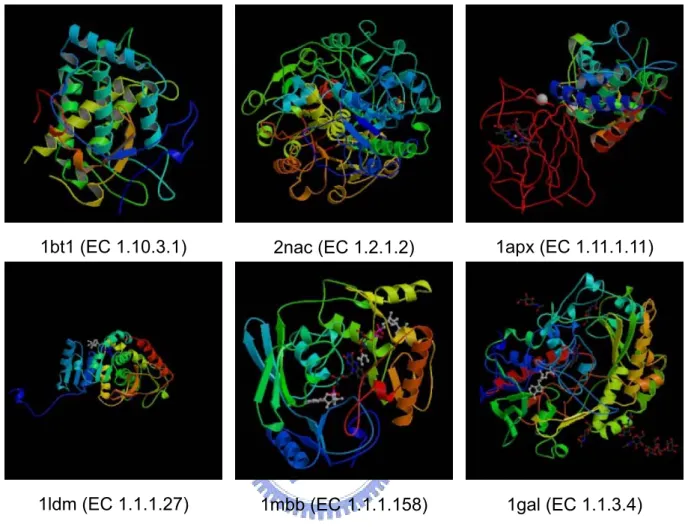
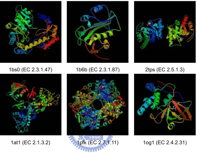
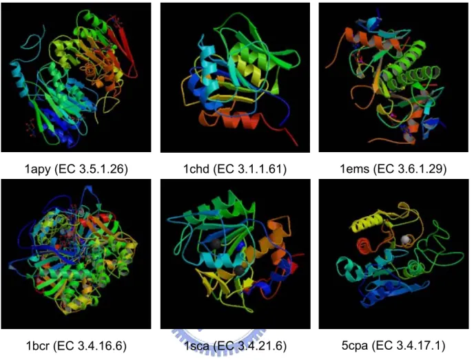
We can take oxidoreductases for example. Here are six structures of some enzymes known as oxidoreductases (EC No. 1) in Figure 2. All these enzymes are classified as oxidoreductases, but they have low structure and sequence similarities with each other which are shown in Table 2, and three of these proteins are even in the same subclass. Since there are no same characteristics found in structures and sequences, we want to check if it is possible to have characteristics in mechanisms. We take three proteins for examples which are classified to the same subclass in Figure 2 to see their mechanisms in the reactions. Here are the reactions of these proteins in Table 3. We can also see the differences in other enzyme class such as in Figure 3 and Figure 4. Methods mentioned above are not useful enough for predicting enzyme class. Because of the diversity of protein structures and mechanisms, we can not use DALI or CASTp to predict enzyme functions. Because of the low sequence similarity between 2 proteins, using PSI-BLAST may not be reliable.

There are some methods to predict enzyme class. Dobson and Doig provided a 2-level SVMs model and the features they used include protein composition, surface protein composition, secondary structures, general protein information, and some metal atoms. They use not only sequence but also structure-based information as

SVM features. In their paper, they can get a 35% accuracy of prediction, but that is not good enough. Here we provide a Huffman tree model in order to get higher accuracy.

DATASET

498 enzymes (Dobson and Doig 2005) have been chosen using function

definitions obtained from DBGet (Fujibuchi, Goto et al. 1997) PDB Enzyme (Bairoch 2000) cross-links and structural relations from the Astral SCOP 1.63 superfamily level dataset. The Astral lists were culled so that only whole protein structures with a SPACI score (Brenner, Koehl et al. 2000) of 0.3 or greater could be selected for each

functional class. The distribution of each enzyme classification is listed in Table 4. All proteins used in this work are listed in Appendix.

These 498 enzymes are taken to do pair wise multiple sequence alignments (MSA) and almost 100% of alignments have less than 20% sequence identity. In each functional class no structure contains a domain from the same superfamily as any other structure.

METHODS

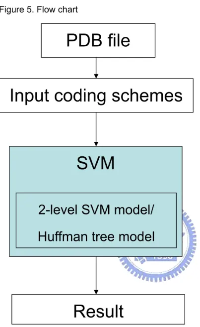
In Figure 5, here is the flow chart which we need to individually introduce every state in order.

Coding schemes

We use both structure-based and sequence-based protein information as our SVM features.

At structure-based protein information part, there is a website

http://www.ebi.ac.uk/thornton-srv/databases/cgi-bin/CSS/makeEbiHtml.cgi?file=form. html which is used to provide us some information as structural protein information.

This catalytic site search (CSS) web server allows us to submit protein structures and search them using the related bank of structural templates(Torrance, Bartlett et al. 2005), in order to identify residue patterns resembling known catalytic sites. Structural templates describe small groups of residues within protein structures, such as the Ser-His-Asp catalytic triad in the serine proteases (see Figure 6). Structural templates can be used with a template searching program to search a protein of unknown function for residue patterns whose function is known. This server uses a library of templates describing catalytic sites, derived from the Catalytic Site Atlas (CSA).

The catalytic site atlas is a database describing catalytic sites in enzymes of known structure. The annotations in the CSA are taken manually from the scientific literature. This annotation is extended to related enzymes in the following manner: the sequence similarity searching program PSI-BLAST is used to search for relatives of the enzymes which have been manually annotated; relatives which have conserved catalytic residues are selected; the catalytic residue annotation is transferred from the manually annotated entries to their selected relatives.

Each literature entry together with its annotated relatives constitutes a CSA family. For each member of a given family, a structural template is constructed representing its catalytic residues. An all-against-all superposition is carried out on templates within the family, in order to determine structural distances between all templates, quantified by RMSD/E-value. The template with the lowest RMSD/E-value from all other family members is the representative template for that family. The representative templates for a non-overlapping set of 147 families are used for searching by this server (shown in Appendix).

All templates are capable of matching similar residue types: Glu can match Asp, Gln can match Asn and Ser can match Thr. Additionally, certain equivalent atom types

can match one another. For example, the two oxygens in the carboxyl group of Glu are chemically equivalent to one another, but have different names in PDB files. They are permitted to match either way around.

This server uses the template matching program Jess(Barker and Thornton 2003) to search for matches to structural templates. Jess does not detect every possible combination of residues within a protein that match to a given template. That would take too much time. Instead, Jess only detects those hits where all inter-atom distances are within 6 Å of the equivalent inter-atom distances in the template. Only the best hit that Jess obtains between a given template and a given protein is reported. A summary of all hits obtained by Jess is provided, in order of E-value. An example of the output is shown as Figure 7. Here are the expansions of each column: hit rank column (hits are ranked by their E-values); template column (each template is based upon an entry in the CSA, which corresponds to a single PDB code); description in PDBsum column (a brief description of the protein structure upon which the template is based); RMSD column (root mean square deviation between the template atoms and the matching atoms in the target); E-value column (the E-value is the number of hits of this quality or better that you would expect to obtain at random. E-values are useful because the statistical significance of RMSD values is not equivalent from one template to another); assessment column (an assessment of how likely the hit is to be meaningful. It is based solely on the E-value. E-value < 1e-8: Highly probable; 1e-8 < E-value < 1e-5: Probable; 1e-5 < E-value < 0.1: Possible; E-value > 0.1: Unlikely); details column (which provides a link to further details of the match, given further down the page); residues in template (which describes the residues in the template structure which matched your query); matching residues in query structure (which shows which residues in your query matched which residues in the template); raw

Jess output (At the bottom of the output page there is a link to the raw output produced by Jess(Barker and Thornton 2003)).

Catalytic site atlas (CSA), a resource of catalytic sites and residues identified in enzymes using structural data, provides catalytic residue annotation for enzymes in the Protein Data Bank. In CSA, many 3-D templates are created as specific 3-D conformations of small numbers of residues. The enzyme active-site templates are used in this work. Each of them consists of one, two or three residues that are known from the literature to be catalytic, plus one or more additional residues whose 3-D positions are highly conserved relative to the catalytic residues. It is available online at

http://www.ebi.ac.uk/thornton-srv/databases/CSA.

Several different protein compositions is used to generate sequence- based information for getting better results on SVM.

A general global sequence descriptor based on the protein composition coding has been used to discriminate protein properties in a number of applications. The coding means the usual amino acid composition. The coding gives the dipeptide composition. We use to denote the partitioned amino acid composition in which the sequence is partitioned into subsequences of equal length, and each fragment

5

den es that the s ence is divided in 5 subsequences, e h of which is en ed by C (note CX is equivalent to ₁ C and we use only _n

C

D

n

YX

n

encoded by the particular amino acid composition . For example, the notation

ot equ to ac cod

that

Y CX

X to substitute CX ). _n

Th

denoted by , in which we compute the composition of the sequence of the form, e coding YX provides information about the local properties of sequences. _n

Another generalized sequence composition is the n -gap dipeptide compositions,

n

( )_n

a x b where a and b enote two specific amino acid types, and ( ) d x denotes _n

intervening amino acids of arbitrary type

n

x. Note that in the special case of n= , 0 is equivalent to .

centered on a given amino acid type. The provides

is the length 0

In addition, we use N C to denote the amino acid composition of a sliding _l

window of leng

Dj D

th l N C_l

information of the flanking sequences of a given amino acid type. Note that when l

L of the whole sequence, N C reduces to _L . This coding schemes are

Besides, we regroup the amino acids into smaller number of classes according to their physico-chemical properties. In this work, we use the following classification schemes

C

list in Table 5.

of the amino acids based on their physico-chemical properties - we use Hn for polar

al. 1999); for small (GASCTPD), medium (NVEQIL) and large (MHKFRYW) (Dubchak, Muchnik et al. 1999);

(RKEDQN), neutral (GASTPHY) and hydrophobic (CVLIMFW) (Dubchak, Muchnik et

V_n

Z_{n for of low polarizability (GASDT)(Dubchak,}

et al. 1999); n for low polarity (LIFWCMVY), neutral (PATGS) and high polarity (HQRKNED) (Dubchak, Muchnik et al. 1999); n for acidic (DE), basic (HKR), p (CGNQSTY) and nonpol

Muchnik et al. 1999), medium (CPNVEQI) and high (KMHFRYW) (Dubchak, Muchnik

olar ar (AFILMPVW);

P

F

S_{n for acidic (DE), basic (HKR), aromatic}

WY), small hydroxyl (ST), sulfur-containing (CM) and aliphatic (AGPILV); for c (FWY), small hydroxyl (ST), sulfur-containing (CM), aliphatic 1 (AGP) and aliphatic 2 (ILV). For clarity, these coding schemes are

sum

Support vector machines

E_n

(F

acidic (DE), basic (HKR), aromati

Support vector machines (SVMs) are a set of related supervised learning methods used for classification and regression. Their common factor is the use of a technique known as the "kernel trick" to apply linear classification techniques to non-linear classification problems.

.

e

ta y

is known as the maximum-margin hyperplane or the optimal hyperplane, as are the vectors that are closest to this hyperplane, which are called the support vectors

Suppose there are some data points which need to be classified into two classes Often we are interested in classifying data as part of a machine-learning process. These data points can be multidimensional points. We are interested in whether w can separate them by a hyperplane (a generalization of a plane in three dimensional space to more than three dimensions). As we examine a hyperplane, this form of classification is known as linear classification. We also want to choose a hyperplane that separates the data points "neatly", with maximum distance to the closest da point from both classes -- this distance is called the margin. We desire this propert since if we add another data point to the points we already have; we can more accurately classify the new point since the separation between the two classes is greater. Now, if such a hyperplane exists, the hyperplane is clearly of interest and

.

We consider data points of the form: where

the c s.

ining data, which denotes the correct classification which we would like the SVM to eventually distinguish, by means of the dividing hyperplane, which takes the form

i is either 1 or −1 -- this constant denotes the class to which the point xi belong

As we are interested in the maximum margin, we are interested in the support v and the parallel hyperplan

ectors es (to the optimal hyperplane) closest to these support vectors in either class. It can be shown that these parallel hyperplanes can be described by equations

We would like these hyperplanes to maximize the distance from the dividing

hyperplane and to have no data points between them. By using geometry, we find the distance between the hyperplanes being 2/|w|, so we want to minimize |w|. To exclude data points, we need to ensure that for all i either

This can be rewritten as:

The problem now is to minimize |w| subject to the constraint (3). This is a quadratic programming (QP) optimization problem.

After the SVM has been trained, it can be used to classify unseen 'test' data. This is achieved using the following decision rule;

Writing the classification rule in its dual form reveals that classification is only a

nction of the Support vectors, i.e. the training data that lie on the margin. Here is the fu

picture in Figure 8 to describe the operation of support vector machines.

n. For w w

VM system comprising 3 classifiers, say,

2-level support vector machine (SVM) model

The first level SVM classifiers comprise a number of separate SVM classifiers, each based on a specific sequence coding as described in the previous sectio the sake of notation simplicity, e ill use the coding symbol to represent the SVM classifier based on that coding. For example, we will denote the S

A, B and by the shorthand symbol . In this work, the first level class sist of the following :

C A+B+C ifiers con SVMs a₁ X_k k=1 9

∑

∑

∑

∑

SVM will generate a probability distribution(Yu, Wang et al. 2003; Yu, Lin et al. 2004 of the subcellular localization based on its particular sequence coding. A second SVM (i.e. the jury SVM) is used to process these probability distributions to gene

)

rate the nal probability distribution and the location with the largest probability is used as the

el SVM system is shown schematically in Figure 9.

the habet, ty of The Huff fi

prediction. The two-lev

Huffman tree model

Because of the unbalanced dataset which would lead to high accuracy but all predictions focusing on just one classification, a Huffman tree model is constructed. Huffman coding is a method of lossless data compression, and a form of entropy encoding. The basic idea is to map an alphabet to a representation for that alp composed of strings of variable size, so that symbols that have a higher probabili occurring have a smaller representation than those that occur less often.

man's algorithm, key to Huffman coding, constructs an extended binary tree (Huffman tree) of minimum weighted path length from a list of weights.

A Huffman tree is a binary tree which minimizes the sum of f(i)D(i) over all leaves i, where f(i) is the frequency or weight of leaf i and D(i) is the length of the path from the root to leaf i. In each of the applications, f(i) has a different physical meaning. Here is an example of Huffman tree in Figure 10. It has the following properties: every internal node

f each leaf mean the number of its enzyme class. According to prev

r, ild

t

ontinue until only one node with no parent remains. That node

a ions; on the

n of has 2 children; smaller frequencies are further away from the root; the 2 smallest frequencies are siblings.

In this work, every leaf on the Huffman tree means the classification of enzymes; the frequencies o

ious statement, we have six nodes (leaves) at beginning and each of them has its own frequency.

The Huffman tree structure contains nodes, each of which contains a characte its frequency, a pointer to a parent node, and pointers to the left and right ch

nodes.The tree can contain entries for all 6 possible leaf nodes and all 5 possible parent nodes. At first there are no parent nodes. The tree grows by making

successive passes through the existing nodes. Each pass searches for two nodes tha have not grown a parent node and that have the two lowest weights. When the algorithm finds those two nodes, it allocates a new node, assigns it as the parent of the two nodes, and gives the new node a frequency count that is the sum of the two child nodes. The next iteration ignores those two child nodes but includes the new parent node. The passes c

will be the root node of the tree. We can see the contribution of the Huffman tree step by step in Figure 11.

The Huffman tree model (see Figure 12) in this work is based on the Huffman tree previously constructed. Every node in this Huffman tree has a corresponding file. At terminal node, the file is made including all data of the enzyme classificat

this node. Besides, each internal node has an additional module. These corre

y ct ew e new root has no child nymore. In the end the enzyme classification of the node the input data finally belongs to means the enzyme classification we predict.

rence

betw , 3,

re n in similar accuracies with the range from 33% to 39%. Here is sponding modules include a SVM training set to help predict the enzyme classification.

Every input data should be put into the Huffman tree model from the tree root. B using 2-classification support vector machines, a decision must be made to predi which child the input data belongs to. Then this child node would be taken as a n tree root, and the steps above would be repeated until th

a

RESULTS

Since there are many coding schemes in the protein structure, which coding schemes can be chosen to predict enzyme classification is important.

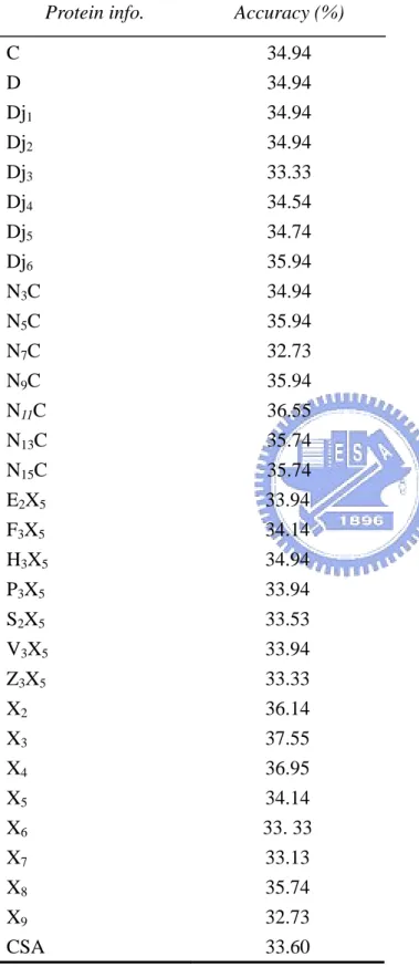
First, we calculate the accuracies of different coding schemes using multi-class SVMs and get the highest performance of 37.55% (shown in Table 7). Although the accuracy is higher than the one from Dobson and Doig, we can see the diffe

een these two: all predictions using multi-class SVMs are biased to EC 1, 2 which class size are largest 3 in six enzyme classes (shown in Figure 13).

Second, we compare with the accuracies of the same method with recent research (Dobson and Doig 2005) but different coding schemes in order to make su if such coding scheme can be used to predict enzyme class. The results are show Table 8. They all have

also accuracies comparison with different coding schemes in each enzyme class shown in Figure 14.

Then, we have to decide which coding schemes are used at each set in the Huffman tree model. Results for the best set accuracies in Huffman tree model with

each of these coding schemes are listed in Table 9. Since pursuing high accuracies in the model is not good enough for this predicting work, we take the best set MCC to

gene f

n

ter s re listed at Table 11. Here is a comparison between the 2-level SVM method

(Dobson and Doig 2005) and the H

n

uracy and un-biased prediction at the same time. Using this model can have a 35% accuracy and a un-biased prediction (Dobson

on

ince the Huffman tree can

deci tree

rate this model. Results for the best set MCC in Huffman tree model with each o these coding schemes are listed in Table 10.

We generate Huffman tree model with different coding schemes at different set, such as C coding in set 7, D in set 8, X2 in set 9, H3X5 in set A, and finally N15C i set B. We pick up coding schemes in every set, some according to set MCC and some according to set accuracy in order to make a set of combinations to get the bet

accuracies in final model. All of combinations and the results for these combination a

uffman tree method in this work in Figure 15.

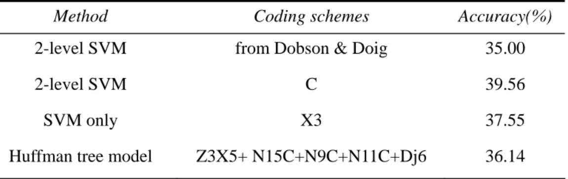
DISCUSSION

Here are accuracies of different methods listed in Table 12 and Figure 16. We ca use only multi-class SVMs to get best prediction of almost 40% accuracy, but the fact is that using multi-class SVMs to predict enzyme class cause the biased prediction. That is why we have to find the other way to do the un-biased prediction. We then use 2-level SVM model in order to get high acc

and Doig 2005) but it seems not enough.

There are some advantages for using Huffman tree model of predicting enzyme classification. Support vector machines are used for 2-classification distinguishing problem at first; all of other SVMs (such as multi-class SVMs) were created based 2-class SVMs which are the simplest and effective classifiers. Predictions by using 2-classification SVMs seem reasonable in this work. S

model is most suitable using 2- classification SVMs.

The dataset in this work is unbalanced with the size of each EC number. Hydrolases, the largest size in this dataset, have 160 out of 498 enzymes (almost one-third) and ligases, the smallest size in this dataset, have only 20 which in size is one-eighth time than hydrolases. The prediction by using multi-class support ve machine would cause the extremely biased prediction, which means all of predicting data may lead to the same enzyme classification, hydrolases, and still get the

prediction accuracy of 33%. Here are the results using mult

ctor i-class SVMs in Table 7. It can can have s. The 5 h. sub- of tree get a 37% above accuracy by guessing only hydrolases and other enzymes which have more members in the dataset like oxidoreductases.

To avoid this biased prediction, Huffman tree model is used to solve the problem with unbalanced size of each classification. Every time we pick two nodes with smallest frequencies and create a new node gathered by these two nodes, we

the assumption following: these two nodes have similarly small frequencie Huffman tree model can balance the size of two children of an internal node.

Two methods are described. One is 2-level SVM (Dobson and Doig 2005) method, which would at beginning separate one multi-classification problem into 1 one-class versus one-class sub-problems, then generate the prediction of the 15 sub-problems by using a one-versus-rest support vector classification approac

Another method is Huffman tree model. We successfully reduce 15 sub-problems to a five-set model. In other words, we can get similar accuracies during only five

problems in this work and it is important because the reduction of the number sub-problems may cause the reduction of the computational time and space.

There are still some advices to get the improvement about the Huffman

model. In Table 9 and Table 10, we can get neither high set accuracy nor set MCC. Although we can not have better prediction in oxidoreductases (EC 1) and

transferases (EC 2), here are the better predictions in hydrolases (EC 3), lyases (EC

4), a of first

tree model we get higher total accuracy.

able 9 n)

his discovery can due to this reason: templates some of which may be useless are sed, and it is necessary to select useful templates to get higher performance.

nd isomerases (EC 5). It tells us as long as we improve the accuracies layer in Huffman

In addition, we can contribute other tree models in order to get better performance.

However, there are still something interesting discovering. In my coding schemes, both sequence-based and structure-based protein information are used. From T

to Table 10, we can find out that using CSA templates (based on structural informatio can not get better performance in our Huffman tree model. In common sense,

structural information is considered more powerful since the same catalytic sites in proteins have more probabilities to be classified to the same enzyme class. T

REFERENCES

Altschul, S. F., T. L. Madden, et al. (1997). "Gapped BLAST and PSIBLAST: a new generation of protein database search programs." Nucl. Acids Res. 25: 3389-3402. Bairoch, A. (2000). "The ENZYME database in 2000." Nucl. Acids Res. 28: 304-305. Barker, J. A. and J. M. Thornton (2003). "An algorithm for constraint-based structural

ng: application to 3D templates with statistical analysis." BIOINFORMATICS template matchi

., S. Naghibzadeh, et al. (2003). "Castp: computed atlas of surface topography

19: 1644-1649.

Binkowski, T. A

of protein." Nucl. Acids Res. 31: 3352-3355.

Brenner, S. E., P. Koehl, et al. (2000). "The ASTRAL compendium for sequence and structure analysis." Nucl. Acids Res. 28: 254-256.

Dobson, P. D. and A. J. Doig (2005). "Predicting Enzyme Class From Protein Structure Without Alignments." J. Mol. Biol. 345: 187-199.

Dubchak, I., I. Muchnik, et al. (1999). "Recognition of a protein fold in the context of the structural classification of proteins (SCOP)." Proteins 35: 401-407.

Fujibuchi, W., S. Goto, et al. (1997). "DBGET/LinkDB: an integrated database retrieval system." Pac. Symp. Biocomput. 3: 681-692.

Holm, L. and C. Sander (1996). "Mapping the protein universe." Science 273: 595-602. Torrance, J. W., G. J. Bartlett, et al. (2005). "Using a Library of Structural Templates to

lytic Sites and Explore their Evolution in Homologous Families." J. Mol. Biol. Recognise Cata

. and A. M. Lesk (2003). "Prediction of protein function from protein

347: 565-581.

Whisstock, J. C

sequence and structure." Q. Rev. Biophys., 36: 307-340.

Xenarios, I., L. Salwinski, et al. (2002). "Dip, the database of interacting proteins: a research tool for studying cellualr networks of protein interactions." Nucl. Acids Res. 30: 303-305.

Yao, H., D. M. Kristensen, et al. (2003). "An accurate, sensitive, and scalable method to identify functional sites in protein structures." J. Mol. Biol. 326: 255-261.

Yu, C. S., C. J. Lin, et al. (2004). "Predicting subcellular localization of proteins for bacteria by support vector machines based on n-peptide compositions." Gram-negative

Protein Sci 13(5): 1402-6.

Yu, C. S., J. Y. Wang, et al. (2003). "Fine-grained protein fold assignment by support vector generalized npeptide coding schemes and jury voting from

ultiple-parameter sets." Proteins machines using

Table 1. The numbers of members and subclass in each enzyme

No. Subclass number Current membesr

TABLES Class 1 Oxidoreductase 22 1286 2 Transferase 9 1245 3 Hydrolase Is 6 Ligase 6 140 13 1385 4 Lyase 7 422 5 omerase 6 167

Table 2. Matrix of sequence identity (colored black) and Z-score (colored red)

c lculate w c r

c x b l

a d bet een ea h othe

1bt1 2na 1ap 1ldm 1mb 1ga 1bt1 7.9 4.2 8.3 3.8 6.9 7.5 2nac 1.6 1gal 2.6 2.3 2.0 2.0 2.3 8.5 8.1 6.2 7.3 5.6 4.2 1apx 3.3 1.6 7.6 15.3 5.6 6.9 1ldm 1mbb 2.0 2.0 4.4 1.2 1.6 2.6 8.0 3.1 8.8 8.0 2.8 2.5

Ta actions of each protein, wh rs drown in red cycle

(EC No.)

Reaction mechanisms

ble 3. Re

PDB ID

ere the reaction occu

1ldm (1.1.1.27) + = pyruvate + NADH + H+ (S)-lactate + NAD 1mbb (1.1.1.158) DP-N-acetylmuramate + NADP (1.1.3.4) + = NADPH + H++ U UDP-N-acetyl-3-O-(1-carboxyvinyl)-D-glucosamine 1gal  

T zyme dataset

E ) Group size

able 4. The size of each en group in the

nzyme Group (EC No.

Oxidoreductases (1) 79 T H ) 160 Isomerases (5) Ligases (6) 20 ransferases (2) 128 ydrolases (3 Lyases (4) 60 51

T

bol

able 5.

Sym Properties Dim

C Protein composition of 20 amino acids 20 D Protein composition of 20 amino acids by 2

continuous amino acids

400 Djn Protein composition of 20 amino acids by 2 amino 400

acids between which there are n other amino acids NnC the amino acid composition of a sliding window of 400

length centered on a given amino acid type. This provides information of the flanking sequences of a given amino acid type

Xn ino acids of n

divisions

n* 20 Protein composition of 20 am

T n 5 able 6. Symbol (U X ) Properties Regr m ouping ember Dim H3X5 Hydrophobicity 135 polar neutral hydrophobic RKEDQN HY GASTP CVLIMFW V3X5 Waals volume W 135 Normalized van der

0.00-2.78 2.95-4.00 4.43-8.08 GASCTPD NVEQIL MHKFRY Z3X5 409 135 Polarizability 0.000-0.018 0.128-0.186 0.219-0. GASDT CPNVEQIL KMHFRYW P3X5 3.0 KNED 135 Polarity 4.9-6.2 8.0-9.0 10.4-1 LIFWCMVY TGS PA HQR F3X5 320 4 groups : acid base r pola nonpolar DE HKR CGNQSTY AFILMPVW S2X5 tic VGP 245 7 groups : acid base amide ic aromat Small hydroxyl r sulfu alipha DE HKR NQ FWY ST CM AIL E2X5 8 groups : 320 acid base amide DE HKR NQ

aromatic small hydroxyl aliphatic 2 ILV sulfur aliphatic 1 FWY ST CM AGP

Table 7. accuracy comparis t coding using multi-class SVMs.

Protein info. Accuracy (%)

on with differen C 34.94 D 34.94 5 5 5 33. 33 9 CSA 33.60 Dj1 34.94 Dj2 34.94 Dj3 33.33 Dj4 34.54 Dj5 34.74 Dj6 35.94 N3C 34.94 N5C 35.94 N7C 32.73 N9 C 36.55 C 35.94 N11 N13C 35.74 N15C 35.74 E2X5 X 33.94 F3 5 34.14 H3X 34.94 P3X5 33.94 S2X5 X 33.53 V3 X 33.94 Z3 33.33 X2 36.14 X3 37.55 X4 36.95 X5 34.14 X6 X7 33.13 X8 35.74 32.73 X

Table 8. Rank accuracy comparison with the same method but different protein information

ative accuracy (%) by rank Cumul Protein info. 1 2 3 4 5 6 Doig 34.94 60.00 77.00 86.00 96.00 100.00 C 39.56 49.84 76.10 89.16 95.98 100.00 D 34.14 60.04 74.50 86.95 95.98 100.00 Dj1 34.34 59.04 74.30 86.95 95.78 100.00 Dj2 33.33 59.44 74.70 87.15 95.98 100.00 Dj3 32.93 58.63 73.29 85.94 95.98 100.00 Dj4 35.54 61.65 75.70 86.35 95.98 100.00 Dj5 32.73 58.23 73.49 83.73 95.78 100.00 Dj6 34.34 59.04 75.70 86.35 95.98 100.00 N3C 31.53 59.44 73.90 85.34 95.98 100.00 N5C C 33.73 61.45 75.30 88.15 95.98 100.00 N7 C 38.35 64.86 79.32 88.15 96.59 100.0 N9 34.14 59.44 74.90 85.94 95.78 100.00 N11C 34.14 59.24 76.91 86.55 95.98 100.00 N13C 33.94 59.44 74.94 85.34 95.98 100.00 N15C X 35.34 61.24 76.91 85.94 95.58 100.00 E2 5 32.73 57.63 73.69 83.94 95.78 100.00 F3X5 33.53 58.03 74.30 87.15 95.98 100.00 H3X5 38.35 61.85 76.10 85.94 95.78 100.00 P3X 5 32.53 58.63 74.30 85.14 95.98 100.00 S2X5 34.14 59.04 74.30 85.34 95.98 100.00 V3X5 X 36.35 61.24 73.69 84.94 95.98 100.00 Z3 5 34.94 62.65 77.31 87.55 95.98 100.00 X2 36.95 61.04 74.10 84.94 95.98 100.00 X3 33.53 62.05 79.12 86.75 96.18 100.00 X4 36.75 61.04 76.31 88.76 95.78 100.00 X5 36.35 60.44 75.90 84.94 95.78 100.00 X6 35.54 60.04 76.10 88.15 95.98 100.00 X7 36.14 63.45 77.71 89.36 95.58 100.00 X8 X 35.34 31.12 61.65 60.24 77.31 75.10 87.75 85.34 95.98 95.98 100.00 100.00 9 CSA 30.32 43.17 61.85 71.89 84.54 100.00

T c y (%) ch pro forma

otein info.

able 9. Set a curac of ea tein in tion

Pr set7 set8 set9 setA setB

C 71.8 61.8 72.5 64.3 59.4 D 73.2 59.5 66.2 65.3 58.6 Dj1 73.2 55.7 69.6 65.6 58.8 Dj2 73.2 61.8 69.1 63.2 59.8 Dj3 73.2 58.0 66.7 63.9 59.4 Dj4 73.2 59.5 65.7 67.4 58.6 Dj5 71.8 55.0 71.0 67.4 59.2 Dj6 73.2 57.3 65.7 64.6 60.4 N3C 73.2 54.2 65.7 65.3 59.0 N5C C 71.8 58.0 68.1 66.7 59.0 N7 C 71.8 59.5 70.0 65.3 58.6 N9 71.8 57.3 71.0 66.3 59.2 N11C 71.8 61.1 68.1 68.7 60.0 N13C 71.8 67.2 69.1 67.4 60.8 N15C X 71.8 61.8 69.1 69.4 60.8 E2 5 73.2 55.7 68.6 64.9 59.0 F3X5 71.8 55.0 63.3 67.4 58.8 H3X5 5 5 9 CSA 73.2 62.3 67.1 59.8 59.4 74.6 59.5 68.1 63.6 58.8 P3X5 73.2 60.3 62.3 64.3 59.0 S2X5 X 74.6 56.5 66.2 65.6 59.4 V3 X 73.2 55.7 69.6 62.9 59.6 Z3 73.2 55.0 67.1 64.6 60.0 X2 71.8 63.4 72.0 66.7 58.4 X3 73.2 58.8 73.4 63.6 59.2 X4 73.2 56.5 74.4 66.3 58.6 X5 73.2 58.0 72.9 66.0 59.0 X6 73.2 58.8 72.0 65.3 58.8 X7 73.2 57.3 69.6 65.3 58.6 X8 71.8 55.7 72.0 64.9 73.2 60.0 58.8 59.6 X 72.5 65.3

T M %) of protein rmatio

otein info.

able 10. Set CC ( each info n

Pr set7 set8 set9 setA setB

C 27.2 19.1 35.8 22.0 13.3 D 19.1 18.8 31.6 27.9 10.8 Dj1 27.2 19.0 33.4 29.7 10.1 Dj2 27.2 18.7 28.2 23.6 11.5 Dj3 19.1 15.2 21.4 23.1 11.0 Dj4 27.2 23.5 24.8 23.6 14.1 Dj5 27.2 18.1 28.3 28.0 12.1 Dj6 19.1 15,7 30.0 30.8 14.4 N3C 14.7 14.8 28.2 25.6 11.3 N5C C 18.0 12.1 34.6 27.1 10.8 N7 C 14.4 19.3 39.3 24.1 8.8 N9 15.3 28.0 37.2 25.4 13.3 N11C 13.2 24.1 37.0 25.3 14.9 N13C 19.1 34.7 35.9 24.0 11.8 N15C X 21.4 30.4 37.0 25.1 17.9 E2 5 19.1 26.2 38.2 25.3 9.6 F3X5 19.0 18.0 15.8 24.5 10.7 H3X5 5 5 9 CSA 10.7 25.7 34.6 19.5 12.4 13.2 23.4 33.6 27.2 11.3 P3X5 20.7 17.4 16.5 23.1 10.8 S2X5 X 28.7 22.3 33.3 29.3 12.1 V3 X 19.1 21.9 30.6 28.8 11.2 Z3 30.5 24.1 27.7 22.1 10.7 X2 19.1 23.0 43.6 28.0 11.9 X3 25.4 17.7 37.9 27.6 13.8 X4 13.2 24.3 45.2 23.1 15.0 X5 13.2 17.2 36.5 23.9 11.9 X6 19.1 15.1 34.6 21.2 12.1 X7 13.2 18.0 31.9 27.4 14.3 X8 19.1 27.3 21.4 16.7 47.2 25.6 34.9 27.6 11.9 11.0 X

Table 11. A odel

C che ifferent set

ccuracies using Huffman tree m

oding s me in d

Set 7 Set 8 Set 9 Set A Set B Accuracy(%)

Z3X5 N13C X4 S2X5 Dj6 34.94 Z3X5 N15C N9C N Z3X5 N15C X2 N11C N15C 35.54 N11C Dj6 36.14 Z3X5 N15C X4 11C Dj6 36.14 Z3X5 N13C X4 Dj6 Dj6 34.34 Z3X5 N13C X4 Dj1 Dj6 34.34 Z3X5 N13C X8 Dj1 Dj6 33.94

Table 12. Accuracy comparison with different methods and different protein informati

Accuracy(%)

on

Method Coding schemes

2-level SVM from Dobson & Doig 35.00 2-level SVM

Huffman tree model Z3X5+ N15C+N9C+N11C+Dj6 36.14

C 39.56

sin

arison with 2 different methods (multi-class SVM

arison with different coding schemes using 2-level

arison with different methods (2-level SVM model

Figure 16. Class accuracies comparison with all methods FIGURE CAPTIONS

Figure 1. The number of proteins with unknown function in PDB Figure 2. Examples of oxidoreductases

Figure 3. Examples of transferases Figure 4. Example of hydrolases Figure 5. The flow chart of this work Figure 6. Example: CSA template of tryp Figure 7. CSS example of the output Figure 8. Support vector machine Figure 9. 2-level SVM

Figure 10. An example of Huffman tree

Figure 11. The construction of the Huffman tree step by step Figure 12. Huffman tree model in this work

Figure 13. Class accuracies comp and 2-level SVM model)

Figure 14. Class accuracies comp SVM method

Figure 15. Class accuracies comp and Huffman tree model)

FIGURES

Figure 1. The number of proteins with unknown function in PDB

The number of proteins with unknown function in PDB

11 12 56 78 233 418 386 121 0 50 100 150 200 250 300 350 400 450 1992-1999 2000 2001 2002 2003 2004 2005 2006

Figure 2.Examples of oxidoreductases

1bt1 (EC 1.10.3.1) 1apx (EC 1.11.1.11)

1mbb (EC1.1.1.158) 2nac (EC 1.2.1.2)

1gal (EC 1.1.3.4) 1ldm (EC 1.1.1.27)

Figure 3. Examples of transferases 1bs0 (EC 2.3.1.47) 2tps (EC 2.5.1.3) 1at1 (EC 2.1.3.2) 1b6b (EC 2.3.1.87) 1og1 (EC 2.4.2.31) 1pfk (EC 2.7.1.11)

Figure 4. Example of hydrolases 1sca (EC 3.4.21.6) 1apy (EC 3.5.1.26) 1bcr (EC 3.4.16.6) 1chd (EC 3.1.1.61) 5cpa (EC 3.4.17.1) 1ems (EC 3.6.1.29)

Figure 5. Flow chart

PDB file

Input coding schemes

SVM

2-level SVM model/

Huffman tree model

Figure 9. 2-level SVM

SVM

Protein

…

Feature selection

Result

SVM

SVM

SVM

v

v

v

…

Figure 11. The construction of the Huffman tree step by step (5)51 (4)60 (1)79 (2)128 (3)160 (6)20 (5)51 (2)128 (3)160 (1)79 (4)60 (6)20 (7)71 (5)51 (2)128 (3)160 (1)79 (4)60 (6)20 (7)71 (8)13

(2)128 (1)79 (9)20 (5)51 (4)60 (6)20 (7)71 (8)13 (3)160 (A)29 (5)51 (4)60 (6)20 (7)71 (8)13 (3)160 (2)128 (1)79 (9)20 (2)128 (1)79 (9)20 (5)51 (4)60 (6)20 (7)71 (8)13 (3)160 (A)29 (B)498

Figure 12. Huffman tree model in this work

8

7

A

B

9

Figure 13. Class accuracies comparison with 2 different methods (multi-class SVM and 2-level SVM model)

0 20 40 60 80 100 1 2 3 4 5 6 only SVM ( X3 )

Figure 14. Class accuracies comparison with different coding schemes using 2-level SVM method 0 20 40 60 80 100 1 2 3 4 5 6 2-level SVM model ( C ) 2-level SVM model ( N7C ) 2-level SVM model ( H3X5 ) 2-level SVM model ( Doig )

Figure 15. Class accuracies comparison with different methods (2-level SVM model and Huffman tree model)

0 20 40 60 80 100 1 2 3 4 5 6

2-level SVM model ( Doig ) Huffnab tree model ( set 1 ) Huffnab tree model ( set 2 )

Figure 16. Class accuracies comparison with all methods 0 20 40 60 80 100 1 2 3 4 5 6 only SVM ( X3 ) 2-level SVM model ( C ) 2-level SVM model ( Doig ) Huffnab tree model ( set 1 ) Huffnab tree model ( set 2 )

APPENDIX Description of each enzyme classification

Group Reaction catalyzed Typical reaction Enzyme example(s) with trivial name EC 1 Oxidoreductases

To catalyze oxidation/reduction reactions; transfer of H and O atoms or electrons

from one substance to another

AH + B → A + BH (reduced) A + O → AO (oxidized) Dehydrogenase, oxidase EC 2 Transferases

Transfer of a functional group from one substance to another. The group may be methyl-, acyl-, amino- or phospate group

AB + C → A + BC Transaminase, kinase EC 3 Hydrolases

Formation of two products from a substrate by hydrolysis AB + H2O → AOH + BH Lipase, amylase, peptidase EC 4 Lyases

Non-hydrolytic addition or removal of groups from substrates. C-C, C-N, C-O or C-S bonds may be cleaved

RCOCOOH → RCOH + CO2

EC 5

Isomerases

Intramolecule rearrangement, i.e.

isomerization changes within a single molecule

AB → BA Isomerase, mutase

EC 6

Ligases

Join together two molecules by synthesis of new C-O, C-S, C-N or C-C bonds with simultaneous breakdown of ATP

X + Y+ ATP → XY + ADP + Pi

Dataset (Oxidoreductases / EC No. 1)

1a8q 1aor 1arx 1b4u 1b5t 1ba3 1bug 1ci0 1cp2 1cpo 1cpt 1cq1 1d4o 1d6u 1d7c 1do6 1dtw 1e1d 1eb7 1en6 1evi 1f0y 1ff3 1fp4 1geu 1goh 1gqh 1h2a 1h4i 1hb1 1hfe 1hlr 1hqt 1htp 1hwj 1i9d 1ik3 1ika 1ikt 1ivj 1jl3 1jpu 1knd 1l1d 1l5t 1l6p 1m41 1me8 1mhc 1mj4 1mro 1ndo 1ndt 1niw 1nox 1oya 1phm 1qav 1qbg 1qdb 1qg0 1qi1 1rx8 1sur 1sxz 1uox 1vao 1vif 1vnf 1xik 2aop 2bbk 2dmr 3mde 3pcm 4nos 5r1r 6pah 8cat

Dataset (Transferases / EC No. 2)

1a59 1a6j 1b4f 1b7b 1bdf 1ble 1bmt 1bo1

1btk 1c2p 1c41 1c4g 1ckn 1cm1 1d0q 1dd9 1dy3 1dzf 1e0c 1e2a 1e2o 1e6v 1efz 1eh8 1ejc 1ep9 1ew0 1eye 1ez1 1ezf 1f0l 1f0n 1f75 1f7t 1f8y 1ffs 1fgg 1ftr 1g0w 1g2p 1g5h 1g6c 1g6g 1g71 1gjv 1gmi 1gms 1gno 1gpb 1gpu 1gq5 1gz0 1h17 1h54 1hav 1hkc

1hml 1hxq 1hzw 1i2n 1ig3 1iib 1ik7 1im8

1iu4 1ixm 1jg9 1jho 1jkx 1k04 1k1f 1k30 1k47 1k9s 1k9v 1kgy 1kgz 1khc 1ki8 1kq4 1kzh 1kzl 1l2q 1ld8 1lii 1liu 1lkl 1lp4 1lqp 1lt8 1m3k 1m4j 1m6b 1m9z 1mby 1ml9

1moq 1msk 1n06 1nh7 1nm2 1nom 1nun 1pdo

1poi 1ptq 1qap 1qd1 1qf8 1qjc 1qsm 1rgs 1shf 1vpe 1vsf 1xat 1xrc 1xtc 1zym 22gs 2a0b 2bef 2can 2cbf 2daa 2f3g 2jdx 2pol

Dataset (Hydrolases / EC No. 3)

1a17 1a2o 1a2t 1a6f 1a6q 1a79 1ak0 1alw

1amp 1aqt 1aug 1auo 1avg 1ayd 1az9 1b65

1b6m 1b79 1b9v 1bgo 1bir 1bpl 1bwr 1c77 1c8u 1ceb 1cel 1cfr 1cfz 1cjy 1cqy 1ctt 1cug 1cvm 1cwt 1d8i 1dix 1dnk 1dup 1dx5 1e1a 1e44 1e7d 1em9 1eni 1eoj 1ewn 1ex1 1f0j 1fce 1fcm 1fo2 1fo6 1fpb 1fw3 1fwg 1g0s 1g2i 1g9z 1gny 1gpp 1gtp 1gye 1gym 1h70 1h8g 1hja 1ho3 1hrt 1hv5 1hxk 1hzf 1i3j 1i3o 1i4o 1i74 1i78 1i8a 1icf 1ici 1ief 1ifs 1ihj 1iod 1iqb 1isj 1iw8 1j98 1j9l 1jh7 1jhc 1jke 1jt9 1jys 1k3b 1k46 1k5c 1k82 1kg7 1khl 1kie 1klx 1ko7 1kvc

1ky4 1l2p 1l7n 1lau 1lba 1lbu 1lkt 1lmh

1ln0 1m9n 1mc0 1mc9 1mml 1mt5 1mu7 1n64 1n8o 1nb3 1nba 1ngh 1nzy 1o0w 1pex 1png 1prx 1ptt 1pvc 1qaz 1qbj 1qcn 1qdn 1qfx 1qk2 1qlm 1qum 1rbd 1scn 1svb 1ush 1wgi 1xo1 2acy 2bqk 2dyn 2kai 2mjp 2phi 2pth 2reb 3bc2 3eng 3pva 3ygs 5pnt 5rla 6fit

Dataset (Lyases / EC No. 4)

1ahj 1ayl 1b66 1b6r 1ca2 1csh 1csm 1d7a 1dch 1dci 1dnp 1doz 1dp4 1dqs 1dwk 1dxe 1e51 1e9n 1ebm 1egh 1et0 1f3t 1fgh 1fi4 1fro 1fuo 1fx4 1gqo 1gxo 1i6o 1i7o 1iv1 1j58 1jbq 1jd3 1jl0 1jr2 1ju2 1juk 1k0e 1k8t 1k8w 1kep 1kiz 1kko 1lk9 1mka 1n7n 1n8w 1nbw 1o8f 1pda 1ppp 1qpb 1qrl 1rus

Dataset (Isomerases / EC No. 5)

1a41 1am2 1amu 1b73 1b9l 1bgw 1bkf 1bkh 1bwz 1com 1cy9 1d3y 1dea 1did 1e59 1eej 1ek6 1epz 1eqj 1eyq 1f2v 1f6d 1fp3 1fui 1g58 1hnu 1i8t 1i9a 1iv8 1j5s 1jc4 1jof 1k0w 1lvh 1lzo 1mx0 1nsu 1nuh 1ois 1pii

1pym 1qjg 1sqc 1vcc 1vkl 2req 2sfp 3gsb

Dataset (Ligases / EC No. 6)

1a48 1a8h 1ayz 1b04 1b47 1bdo 1cg1 1cli 1ct9 1d5f 1e4e 1eeh 1h4s 1htq 1i2t 1ik9 1mdb 1mkh 1qmh 1ycr

Representative CSA templates for a non-overlapping set of 147 families

12as 1km1 1c1h 1hz1 1gal 3fit 1b8a 1kdn 1fmt 1oya 1ql0 1kkt 1avw 1wab 1d8w 1pgn 1qgy 1xid 1a2f 1dnw 1afr 1nux 1lam 3er3 1k9z 1ucc 1d8h 2nac 1l1n 1pnt 1lta 1cy8 1osj 1jf9 1hbz 1cjw 1cg0 1f3t 1raf 1gxz 1gpi 4pfk 2lip 2dnj 1kf4 1hmp 1hl2 1ryb 1foh 5csm 1apy 1knf 1m1t 1jep 1pzh 1bcr 1zrm 1nwc 1kta 2npx 1gpf 1pow 2ayh 1ei9 1ndz 6enl 1dd8 1edd 1ftw 5yas 1aur 1onr 1chd 1pfq 1naw 1owp 1h1y 1vgv 1egm 1djq 1nf5 3nse 1ghs 1ah3 1aj0 1pyd 1brl 1bd4 1bvw 1dj9 1dah 1b0p 1cwy 1n7n 1iov 1qnt 1k7x 1qtq 1e2h 1b73 1gpr 1jp3 2ay6 1opm 1cns 1pj5 3uag 1pj4 1yjb 1gpk 1diz 2tps 1g9r 1hdq 1os1 1um9 1csc 1gon 1mas 1jz7 1qpq 1nyy 1dcp 1h17 1nhc 1f61 1dty 1mbb 1gyc 1bg4 1fwc 1b8f 1h7p 1gqn 1uou 1f17 1n1p 1say 1a9s 1ecj 1sry 1hor 1djl 1qfm