3D Reconstruction and Face Recognition Using Kernel-Based
ICA and Neural Networks
Cheng-Jian Lin Ya-Tzu Huang Chi-Yung Lee
Dept. of Electrical Dept. of CSIE Dept. of CSIE Engineering Chaoyang University Nankai Institute of
National University of Technology Technology of Kaohsiung s9527618@cyut.edu.tw cylee@nkc.edu.tw
cjlin@nuk.edu.tw
Abstract
Kernel-based nonlinear feature extraction and classification algorithms are popular research topics in machine learning. In this paper, we propose an improved photometric stereo scheme based on the basic reflectance model. In order to reconstruct a human face as a 3D model, we use kernel independent component analysis (KICA) to obtain the face’s surface normal vector on each point of the image. In this procedure, we find that the x-axis, y-axis and z-axis values of the normal vector’s coordinates are not arranged in order. Thus, an improved KICA (IKICA) method is proposed that takes the normal vector of a synthetic spherical surface normal vector as the supervised reference for solving this problem. After obtaining the correct normal vector’s sequence form surface, we use a method for enforcing integrability to reconstruct 3D objects. We test our algorithm on synthetically generated images to reconstruct object surfaces on a number of real images captured from the Yale Face Database B, and use three kinds of methods to fetch characteristic values. Those methods are called contour-based, circle-based, and feature-based methods. Then, a three layer feed-forward neural network trained by back-propagation algorithm is used to realize a classifier. All the experimental results were compared to those of the existing human face reconstruction and recognition approaches tested on the same images. The experimental results demonstrate that the proposed improved kernel independent component
analysis (IKICA) method of reconstruction and human recognition are efficient approaches.
Keywords: Independent component analysis, 3D human face reconstruction, 3D human face recognition, back-propagation algorithm, neural networks.
1. Introduction
When we use a camera to capture 3D objects, we lose the depth information of the 3D objects and only obtain the 2D image information. However, the depth information of the 3D objects plays an import role in many applications, such as 3D object recognition and 3D object display. In order to show the original information of the 3D objects, the problems of reconstructing 3D objects from 2D images need to be resolved. One of the approaches to computer vision is the photometric stereo approach to surface reconstruction. This approach is able to estimate the local surface orientation by taking several images of the same surface from the same viewpoint but under illuminations from different directions. The main limitation of the classical photometric stereo approach is that the light source positions must be accurately known. This necessitates a fixed, calibrated lighting rig. Hence, an improved photometric stereo method for estimating the surface normal and the surface reflectance of objects without a priori knowledge of the light source direction or the light source intensity was proposed by Hayakawa [1]. Hayakawa’s method uses the singular-value
decomposition (SVD) method to factorize an image data matrix of three different illuminations into a surface reflectance matrix and a light source matrix based on the Lambertian model. However, Hayakawa still uses one of the two added constraints for finding the linear transformation between the surface reflectance matrix and the light source matrix. McGunnigle [2] introduced a simple photometric stereo scheme, which only considered a Lambertian reflectance model, where the self and cast shadows, as well as the inter-reflections, were ignored. Three images at a tilt angle of 90∘increments were captured. McGunnigle suggested using his method as a first estimate for an iterative procedure.
Lin et al. also proposed a novel ICA-based photometric stereo approach based on a non-Lambertian model [3]. The goal of the ICA model is to separate the independent component of a surface normal at each point of an image. But the ICA model still has the problem of the x-axis, y-axis and z-axis values of the separated normal vector not being arranged in order. Thus, a constrained independent components analysis (cICA) model [4][5] was proposed. It is a supervised ICA model which may arrange the outputs of a normal vector’s coordinate values in order. Thus, Lee et al. proposed a cICA-based photometric stereo reconstruction method to solve the normal vector disorder problem [6]. But we find that the cICA model has other problems. Generally, the input data which we feed into the cICA model are linear data. Actually, the input data that we obtain from 2D images are non-linear. Thus, all the non-linear data must be changed into linear data first before the cICA process is used. But this transformation would unavoidably cause some distortion. One kind of linear transformation method that we utilize kernel algorithm [7][8]. It does not need to know the necessary parameter in the linear transformation, and enable us to transform smoothly and fast.
In this paper, an improved kernel
independent component analysis (IKICA) method is proposed to take the normal vector of a synthetic spherical surface as the supervised reference. The proposed IKICA extends the traditional kernel independent component analysis (KICA) model [9]-[13]. It is a non-linear ICA model which can directly transform non-linear data from 2D images. Therefore, introductory data do not need to undergo linear conversion in advance. Thus, the proposed model can reduce the number of normal vector errors of 3D objects effectively. The 3D surface model is then reconstructed from the surface normal at each pixel of an image, obtained by using the IKICA technique and a method for enforcing integrability [14]. The reason for using these methods is that they are easy to implement. After using reconstructive method, we get lots of 3D human faces as our 3D database. Therefore we fetch the 3D information of 3D face model to make 3D human recognition.
The rest of this paper is organized as follows. The details of the proposed IKICA-based reflectance model and its derivations are presented in Section 2. We present the 3D model reconstruction in Section 3. After face reconstruction, we discuss with 3D face recognition in Section 4. Experimental results are given in Section5. The last Section describes the conclusions.
2. The improved KICA model
2.1 The KICA modelICA is a technique that transforms a multivariate random signal into a signal having components that are mutually independent in the complete statistical sense [4]. Let the time-varying observed signal be
, ) , , , ( 1 2 T m x x x K =
x and the desired signal
consisting of independent components (ICs)
be T n s s s , , , ) ( 1 2 K =
s . The classical ICA
assumes that the signal x is an instantaneous linear mixture of ICs, or independent sources si,i=1,2,...m. Therefore, x=As, where
the matrix A of size n×m represents the
goal of the ICA is to obtain a m×n
demixing matrix W to recover all the ICs of
the observed signal. T
m
y y y
y=( 1 , 2 ,K , ) is given by y=Wx. For simplicity, in this section, we address the case of a complete ICA, in which n=m.
The main idea of KICA is to map the input data into an implicit feature space F firstly: Φ:x∈RN →Φ(x)∈F. Then KICA is
performed in F to produce a set of nonlinear features of input data. As ICA algorithm described in the above part, the input data X is whitened in feature space F. The
whitening matrix is: T
V W~ ( )2( ) 1 Φ Φ Φ = Λ , here Φ
Λ , VΦ are the eigenvalues matrix and
eigenvectors matrix of covariance matrix
∑
= − Φ Λ = Φ = n i T n X K C 1 1 1 ( ) ( ) ˆ α , respectively. Then we can obtain the whitened data WXΦ as K X W XWΦ =(~Φ)TΦ( )=(ΛΦ)−1αT (1)
where K is defined by : Ky&&:=(Φ(xi)⋅Φ(xj)) and α is the eigenvectors matrix of K. After the whitening transformation, the learning algorithm calculated by the following iterative algorithm: , ~ Φ Φ Φ =W X Y (2)
[
( 1 )]
(~ ) , 2 Φ Φ + Φ = + − −Φ ΔW J J Y TW eY (3) Φ Φ Φ Φ =W + ΔW →W W~ ρ (4)until WΦ converged, and ρ is a learning
constant. According to the above algorithm, the feature of a test data s can be obtained by: ) , ( ) ( 1 s X K W y − αT Φ Φ Λ = (5) where T ns x k s x k s x k s X K( , )=[(1,),(2,),L( ,)] , k is a kernel function.
In the above iteration algorithm, the function Ф is an implicit form. The kernel function k can be computed to instead of Ф.
This trick is named as kernel trick. Many functions can be chosen for the kernel such as polynomial kernel:
k(x,s)=(x⋅s)d (6) Gaussian kernel ( , ) exp( 2 )
2 2σ s x s x k = − − and
sigmoid kernel k(x,s)=tanh(k(x,s)+θ). Liu
and Cheng et al use a cosine kernel function [12] derived from the polynomial kernel function as shown in Eq.(6), which can give a better performance than the polynomial kernel function for feature extraction:
) , ( ) , ( ) , ( ) , ( ˆ s s k x x k s x k s x k = (7) where k is a polynomial kernel. Practically speaking, Kernel-ICA = Kernel-Centering+ Kernel-Whitening+ ICA. Selecting an appropriate kernel function for a particular application area can be difficult and remains largely an unresolved issue. Any new kernel function derived from the kernel k( sx, )
with form kˆ(x,s)=c(x)c(s)k(x,s), has been proved to be a valid kernel function when
) (x
c is a positive real valued function of x, which is always satisfied. So, the cosine kernel is a valid kernel function. We adopt cosine kernel in our experiments.
2.2 The IKICA model
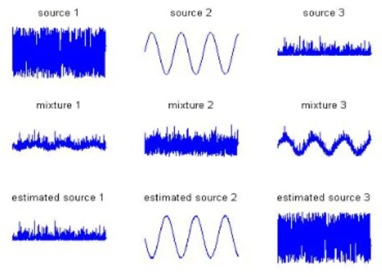
Our previous research used the KICA model to solve the problem of finding the surface normal on each point of an image. But in the KICA model, it is easy to see that the following ambiguities exist in Fig.1: (1) We cannot determine the variances (energies) of the independent components; and (2) We cannot determine the order of the independent components. We generally discover that finding the surface normal vector involves the two problems. For those reasons, we use a constrained learning adaptation algorithm (IKICA) based on image intensities to handle these ambiguities.
Figure 1. “Ambiguities of KICA model.” The source signals are shown in first row, mixing underlying sources shown in second row, and
estimated sources shown in third row.
The IKICA algorithm described in [5] brings in the use of a constraint which is used to obtain an output that is statistically independent of other sources and is closest to a reference signal r(t). This constraining signal need not be a perfect match but it should be enough to point the algorithm in the direction of a particular IC spanning the measurement space. The closeness constraint can be written as
0 ) ( ) (w =ε w −ξ ≤ g (8)
where w denotes a single demixing weight vector such that y=wTv;ε(w) represents the
closeness between the estimated output y and the reference r, andξ represents some closeness threshold. The measure of closeness can take any form, such as mean squared-error (MSE) or correlation, or any other suitable closeness measure. In our implementation of the algorithm, we use correlation as a measure of closeness such that g(w) becomes 0 )} ( { ) (w = −E r w v ≤ g ξ T (9)
where ξ now becomes the threshold that defines the lower bound of the optimum correlation.
With the constraint in place, the IKICA problem is modeled as follows:
Maximize: f(w)=ρ[E{G(wTv)}−E{G(v)}]2
Subject to: g(w)≤0,h(w)=E{y2}−1=0 and
0 1 } { 2 − = r E (10)
where f(w) denotes the one-unit IKICA contrast function; g(w) is the closeness constraint; h(w) constrains the output y to having a unit variance; and the reference signal r is also constrained to having a unit variance. In [5], the problem of Eq.10 is expressed as a constrained optimization problem which is solved through the use of an augmented Lagrangian function, where learning of the weights and the Lagrange parameters is achieved through a Newton-like learning process.
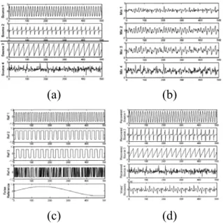
For example, the IKICA algorithm was tested using a synthetic data set of four known sources, as shown in Fig.2(a), which was used for the IKICA work. The sources were linearly mixed by a randomly generated mixing matrix, producing the data set shown in Fig.2(b). With this mixture of data, the IKICA algorithm was run 100,000 times, each time with one of the five reference signals shown in Fig.2(c) as a reference. The first four of these references were obtained from the sign of the four original sources. These were purposely kept as coarse representations of the true sources. The fifth reference is a sine wave which has a frequency radically different than that of any of the original sources, allowing study of the algorithm’s behavior given a “false” reference. Typical outputs of the algorithm are depicted in Fig.2(d). Thus, if we want to find the surface normal vector at each point of an image, we can use the IKICA model.
Figure 2. (a) The four underlying sources of the synthetic dataset. (b) The linearly mixing underlying
sources shown in (a). (c) The different references used for executions of IKICA on 4 channels of data in
(b). The first four references are derived from the signs of the four underlying source, the fifth reference is a “false” reference. (d) Examples of each
recovered source using only the references given in (c), the fifth recovered source shows a “mixture” of
two underlying sources.
3. 3D model reconstruction
3.1 Determining the surface normal of objects using the IKICA modelSuppose that the recovering of surface shape, denoted by z
( )
x ,y , from shadedimages depends upon the systematic variation of image brightness with surface orientation, where z is the depth field, and x and y form the 2D grid over the domain D of the image plane. Then, the Lambertian reflectance model used to represent a surface illuminated by a single point light source is written as:
( ) ( )
(
x ,y , x ,y)
max{
L( )
x ,y( )
x ,y ,0}
R n α = α sTn
∀ ,x y∈D (11)
where R(.) is reflectance component intensity, α
( )
x,y is reflectance albedo on position( )
x,y of surface, s is a column vector indicating the direction of point light, and L is light strength. The surface normalon position
( )
x,y , denoted by n( yx, ), can be represented as( )
( )
[
]
( )
( )
T y x q y x p y x q y x p y x 1 , , 1 , , ) , ( 2 2 + + − − = n (12) where p( yx, ) and q( yx, )are the x- and y-partial derivatives of z
( )
x ,y , respectively.In Eq.(11), max{⋅} sets all negative components that correspond to the surface points lying in attached shadow to zero, where a surface point
( )
x,y lies in an attached shadow iff n(x ,y)s<0 [15].In this section, we describe the method of applying the IKICA model to estimate the normal vector n( yx, ) on the object surface corresponding to each pixel in an image. Since the n( yx, ) vector is a 3×1 column vector, we need at least three images under illumination from lights coming from different directions for the normal vector
) , ( yx
n estimation. Hence, to reconstruct the
3D surface of an object using its images, we have to take three gray-value images under three different illuminants. Assuming an image contains T pixels in total, we can rearrange all the gray values of the three images into a 3×T matrix, with each row representing an image, and each column representing the gray values of a single pixel under three different illuminants. When this matrix is put into Eq.(11), and Eq.(11) is compared with x=As, we find that s is the
) , ( yx
n vector that we are looking for.
Using the IKICA decomposition, we rewrite equation Eq.(11) in matrix form as
) ( ˆ ˆ ) ( ) ( ) (i As i i An i x = =α (13) where 1 3 2 1, , ] ˆ [ ˆ = = − W T a a a A is the matrix
depending on the lighting and viewing directions and has unit length; nˆ t() is the estimated normal vector corresponding to the tth pixel, i = 1, 2, …, T; and α(i) is the
albedo of the ith pixel. However, the decomposition in Eq.(13) is not unique. If there is an invertible matrix G, which (a) (b)
satisfies G A A= ˆ and () 1ˆ() i i G n n = − (14) where A is the true matrix depending on the lighting and viewing directions of the images, and n(i) is the normal vector of the ith pixel in the standard XYZ coordinates, then the linear ambiguity belongs to the subset of GBR [16]-[18]. On the one hand, according to Georghiades’s [18] studies, if the surface of an object is seen under variable light directions, but with a fixed viewpoint, then the linear ambiguity can be reduced to three GBR parameters. As far as the surface normal vectors are concerned, we can only recover n≅G−1nˆ, and ⎥ ⎥ ⎥ ⎦ ⎤ ⎢ ⎢ ⎢ ⎣ ⎡ − − = − 1 0 0 0 0 1 2 1 3 3 3 1 g g g g g G (15) where gi are the three GBR parameters. On the other hand, the three light sources corresponding to the three images do not lie in the same plane (non-coplanar); therefore, the columns of matrix A are linearly independent. In addition, using the IKICA decomposition in Eq.(13), we can obtain an independent basis matrix Aˆ ; thus the ambiguity can further be denoted by a diagonal matrix, i.e., g1 = 0 and g2 = 0. The relation, then, between the normal vectors in the standard XYZ coordinates and those in the independent coordinates system differs only by the g3 factor. For the performance evaluation of 3D image reconstruction, both estimated surfaces and synthetic surfaces are normalized within the interval [0, 1]. Therefore, the influence of the g3 factor on the estimated 3D surface can be removed. 3.2 3D surface reconstruction using the method for enforcing integrability
In this section, we discuss using the method for enforcing integrability to obtain detailed information for reconstructing the surface of an object using its normal vectors. This approach was proposed by R. T.
Frankot and R. Chellappa [14].
Suppose that we represent the surface
( )
x yz , by the functions φ
(
x ,y ,ω)
so that
( )
( ) (
ω ω)
ω , , ,y c x y x z∑
φ Ω ∈ = (16) where ω=( )u ,v is a two-dimensional index,Ω is a finite set of indexes, and the members of
{
φ(
x ,y ,ω)
}
are notnecessarily mutually orthogonal. We choose the discrete cosine basis so that
{
ωc( )
}
isexactly the full set of discrete cosine transform (DCT) coefficients of z
( )
x ,y . Since the partial derivatives of the basis functions φx(
x, y,ω)
and φx(
x, y,ω)
areintegrable, the partial derivatives of z
( )
x ,y are guaranteed to be integrable as well; that is, zxy( )
x,y =zyx( )
x,y.. Note that the partialderivatives of z
( )
x ,y can also be expressed in terms of this expansion, giving
( )
( ) (
ω
ω
)
ω,
,
,
y
c
x
y
x
z
x∑
φ
x Ω ∈=
(17)( )
( ) (
ω
ω
)
ω,
,
,
y
c
x
y
x
z
y∑
φ
y Ω ∈=
(18) where φx(
x,y,ω)
=∂φ( )
⋅ ∂x and(
x y)
( )
y y =∂φ⋅ ∂ φ , ,ω .Suppose we now have the possibly non-integrable estimate n( yx, ) from which we can easily deduce from Eq.(5) the possibly non-integrable partial derivatives
( )
x yzˆx , and zˆy
( )
x,y . These partial derivatives can also be expressed as a series, giving( )
( ) (
ω
ω
)
ω,
,
ˆ
,
ˆ
x
y
c
1x
y
z
x∑
φ
x Ω ∈=
(19)( )
( ) (
ω
ω
)
ω,
,
ˆ
,
ˆ
x
y
c
2x
y
z
y∑
φ
y Ω ∈=
(20)This method can find the expansion coefficients c
( )
ω given a possibly non-integrable estimate of surface slopes( )
x y zˆx , and zˆy( )
x,y : ( ) ( ) ( )( ) ( ) ( )( ) ω ω ω ω ω ω ω y x y x p p c p c p c + + = ˆ1 ˆ2 for ω=( )u,v∈Ω(21) where,( )
(
x
y
)
dxdy
p
xω
=
∫∫
φ
x, ω
,
2 (22)( )
(
x y)
dxdy py ω =∫∫
φ
y , ω, 2 (23) In the end, we can reconstruct an object’s surface by implementing the inverse 2D DCT on the coefficient c( )ω .4. 3D Human face recognition
We success in reconstructing 3D human faces which are used to be 3D face database for human face recognition. There are the three methods which are proposed by us for characteristic values fetching. The neural network is used as classifier to discriminate the 3D face characteristic value of 3D human face database. In order to adjust the parameter of the neural network efficiently, we used back-propagation as a learning algorithm. The detail of the neural network and back-propagation is described in follows.4.1 Method of characteristic fetech
In our system, in order to extract the characteristic value of 3D human faces, three type of fetching methods are defined. Then, we classified the characteristics by back-propagation learning network to complete 3D human face recognition. We would state the three kinds of characteristic value fetching methods separately in following section.
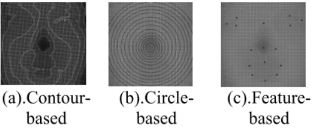
4.1.1 Contour-based fetching method We can get the coordinate value of the
human image every pixel in 3D picture, we fetch z coordinate from it that is the depth of faces of people. In the depth of 3D frontal face, we can be found a supreme point in person's 3D face model which is the so-called nose tip. We utilize the deep relation of 3D faces of people, accord with its deep size, and draw up contour map such as it. We suppose all numbers of value in every contour is n, every deep value is X, and each contour have j pieces of X. The method that we get ith characteristic value is
∑
= = n j j i X contour 1 (24)4.1.2 Circle-based fetching method
First, we fetch z coordinate from 3D human face that is the depth of faces of people. In the depth of 3D frontal face, we can be found a supreme point in person's 3D face model which is the nose tip. Regard nose tip as the centre of a circle, make the radius of the proportion of 3D human face, and draw a round of k in order. There is r a number of deep values in a round of k separately. The q order point depth is Y in each circle of deep value. We adds these deep values which written as
∑
= = r q q k Y Sum 1 (25) Then, we fetch necessary k a characteristic value on average r pieces of Sum valuer Sum
Circle k
k = (26)
4.1.3 Feature-based fetching method Many researchers have investigated facial feature extraction from a frontal view. A number of manual feature extraction algorithms have been proposed, from frontal views, mostly for facial animation [19-22]. Ref. [19] manually picks five feature points from two images to deform a generic mesh model. Ref. [21] relies on manual feature extraction for synthesizing realistic facial
expression from video. Ref. [22] uses stereo frontal images of the face to compute the depth of manually picked feature points. Ref. [23] extracts the centers of the eyes and mouth based on head motion in video frames and knowledge about the facial geometry. Ref. [24] elaborates on the work of Ref. [23] and extracts the corners of the eyes and mouth using template matching for each corner. Ref. [25] utilizes two views of the face and only extracts automatically the pupils’ centers from the frontal view image based on eye template and pupil detector. Ref. [26] uses similar algorithm as Ref. [25] but estimates the 3D points of each feature from two 2D points from each view. The tip of the nose, chin, and upper and lower lip feature points are determined by tracking local maximum curvature at the profile view.
In this section, we automatically extract 15 corresponding facial feature points from the frontal view. These features are landmark points chosen based on their importance in representing a face. Fig.3(c) shows the facial features considered in this section for the frontal view. We measure the nose tip point to the distance of eyes (six points), the nose (three points), the mouth (six points) regards as characteristic value for 3D human face recognition system.
(a).Contour-based (b).Circle- based (c).Feature- based Figure 3. The Three characteristic value fetching
methods of 3D human face.
4.2. The structure of multi-layer neural networks
Multi-neural network is the science of investigating and analyzing the algorithms of the human brain, and using the similar algorithm to build up a powerful computational system to do the tasks like pattern recognition, identification, controlling of dynamical system, system
modeling, and nonlinear prediction of time series. The multi-neural network owns the capability, to organize its structural constituents, the same as the human brain. So the most attractive character of multi-neural network is that it can be taught to achieve the complex tasks.
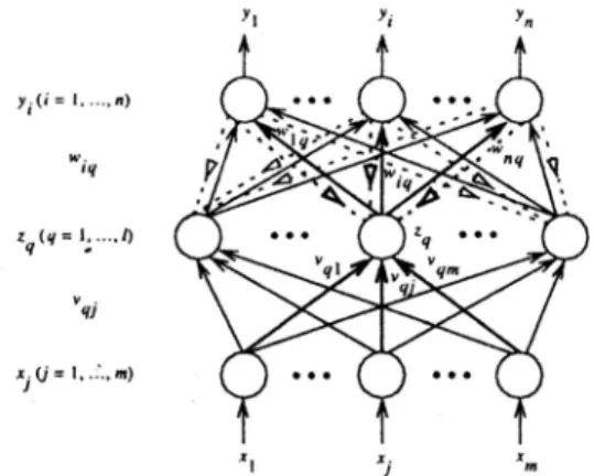
We use a simple three-layer multi-layer neural network as shown in Fig.4 for 3D face recognition. In Fig.4, we have m PEs in the input layer, I PEs in the hidden layer, and n PEs in the output layer; the solid lines show the forward propagation of signals, and the dashed lines show the backward propagation of errors.
Let us consider an input-output training pair (x, d), where the superscript k is omitted for notation simplification. Given an input pattern x, a PE q in the hidden layer receives a net input of j m j qj q
v
x
net
∑
==
1 (25)and produces an output of
( )
⎟⎟ ⎠ ⎞ ⎜⎜ ⎝ ⎛ = =∑
= j m j qj q q a net a v x z 1 (26)the net input for a PE i in the output layer is then ⎟⎟ ⎠ ⎞ ⎜⎜ ⎝ ⎛ = =
∑
∑
∑
= = = j m j qj l q iq q l q iq i w z w a v x net 1 1 1 (27)and it produces an output of
( )
⎟⎟ ⎠ ⎞ ⎜ ⎜ ⎝ ⎛ ⎟⎟ ⎠ ⎞ ⎜⎜ ⎝ ⎛ = ⎟⎟ ⎠ ⎞ ⎜⎜ ⎝ ⎛ = =∑
∑
∑
= = = j m j qj l q iq q l q iq i i a net a w z a w a v x y 1 1 1 (28)Figure 4. Three-layer multi-layer neural network. Transfer function is to do a input weighting value of input of the neuron the summation and is transferred to a kind of mapping rule that is outputted in the function of neural network, influence a kind of design that is channeled into the network of the non-linear one too.
The Back propagation neural network most frequently used non-linear transfer function is sigmoid function. So we use sigmoid function Eq.(29) as transfer function. x e x f − + = 1 1 ) ( (29) 4.3. Back-propagation learning method
The back-propagation learning algorithm [27] is one of the most important historical developments in neural networks. It has reawakened the scientific and engineering community to the modeling and processing of many quantitative phenomena using neural networks. This learning algorithm is applied to multilayer feed forward networks consisting of processing elements with continuous differentiable activation functions. Such networks associated with the back-propagation learning algorithm are also called back-propagation networks. Given a training set of input-output pairs {(x(k) , d(k))}, k=1, 2, …, p, the algorithm provides a procedure for changing the weights in a back-propagation network to classify the given input patterns correctly. The basis for this weight update algorithm is simply the gradient-descent method as used for simple
perceptrons with differentiable units. Back-propagation algorithm has been widely adopted as a successful learning rule to find the appropriate values of the weights for NNs. Generally speaking, because we use the back-propagation learning algorithm, so the error quantity must propagate through time from a stable state to initial state.
For a given input-output pair (x(k), d (k)), the back-propagation algorithm perfo rms two phases of data flow. First, the i nput pattern x(k) is propagated from the input layer to the output layer and, as a result of this forward flow of data, it p roduces an actual output y(k). Then the error signals resulting from the difference between d(k) and y(k) are back-propaga ted from the output layer to the previous layers for them to update their weights. The above section’s equations indicate t he forward propagation of input signals t hrough the layers of neurons. Next, we c onsider the error signals and their back propagation.
In order to make the neural network works properly, we need to find the weights and biases by the learning algorithms. In this study, the supervise learning is used. The network is given a set of training data which contains a number of input pattern and corresponding target output. The learning objective is to reach the high accuracy of classification by minimize the error between target output and network output in the training set. Furthermore, the trained classifier also should to provide a good performance in the untrained data (testing set).
5. Experimental results
We implemented each method in Matlab 7.0 software on a 1.8GHz K8-based PC with 1024 MB RAM According to the results. For 3D reconstruction, we tested the algorithm on a number of real images from the Yale Face Database B [28] showing variability due to illumination. There are varying albedos in each point of the surface
of the human faces. First, we arbitrarily took from these test images the images of the same person who was photographed under three different light sources, as shown in Fig.8. We fed the normalized images into our algorithm. For the face surface reconstruction problem, the normal vectors of a sphere’s surface were used as the reference values for the IKICA model due to their similar structures. The true depth map of the synthetic sphere object is generated mathematically as
( )
⎪⎩ ⎪ ⎨ ⎧ − − + ≤ = otherwise , 0 if , , 2 2 2 2 2 2 r y x y x r y x z (41) where r=48, 0<x ,y≤100, and the center is located at (x, y)=(51, 51). The sphere object is shown in Fig.5. Fig.6 shows the normal vectors of a sphere’s surface.Figure 5. Synthetic sphere surface object.
(a)
(b)
(c)
Figure 6. The normal vectors of a sphere’s surface (a) the X-component, (b) the Y-component, and (c)
the Z-component of the normal vectors.
(a) (b) (c)
(d) (e) (f) Figure 7. (a)-(c) Three training images with
different light source positions from Yale Face Database B [28] in frontal. (d)-(f) Surface normal
corresponding to the three source images.
(a) (b) Figure 8. (a) The surface albedo of human face in Fig.6. The results of 3D model reconstruction by (b)
our proposed algorithm.
After updating the parameters by several iterations, we obtained the normal vector of the surfaces of the human faces corresponding to each pixel in the image in the output nodes. The results are shown in the second row in Fig.7, which give the X-component, the Y-component, and the Z-component of the surface normal vector in order. Fig.8(a) shows the surface albedo of the human face shown in Fig.7. Fig.8(b) shows the result from using our proposed reconstructive algorithm.
Third, the data set in the Yale Face Database B [28] is also used in our experiments for objective comparison. The database consists of 3D face coordinate data and their corresponding 2D front view. Fig.9 shows 6 individuals in the database with 160*160 image size. The results of 3D model reconstruction by our proposed algorithm are showed in second row.
(1)
(2)
(a) (b) (c) (d) (e) (f) Figure 9. (1) Six individuals in the Yale Face Database B [28] used to test our algorithm (these images include
both males and females.). The results of 3D model reconstruction by (2) our proposed algorithm (second row). For face recognition, we propose three
effective algorithms for 3D human face recognition by back-propagation neural networks. We use Yale face database B [28] for reconstruction that provide the geometric properties of 3D face database. The Yale database B contains 10 people faces and each person has 50 2D images, per image is taken under different directions of source light. Therefore 1 person make 10 3D images, 100 3D images regard our 3D database as altogether. We take 50 3D images regard as training data, 50 3D images regard as test data in our 3D database for back-propagation learning network.
The number of the input nodes is defined by the number of characteristic values. Since the 3D face recognition is classified to ten persons, we set the ten output nodes y1-y10 corresponding to each person, respectively. If an input pattern is given, we expect that the value of the output node which is corresponding to the mental category of input pattern is near to 1, otherwise is near to 0. When an unknown data inputs to the network, we can determine which mental task the data belongs to by find the index of maximum value in the ten output nodes. In order to make the output value between 0 and 1, the sigmoid function Eq.(39) is used as the activate function.
Pick the method of fetching in three characteristics that we propose, extract 15 pieces of characteristic value as inputs separately for training. Back-propagation trains each 3D faces independently, it is adequate to recognition applications in
which a model base is frequently updated. For the evaluation of a neural network, the root-mean-square-error (RMSE) is used to compute the average output error
∑ ∑
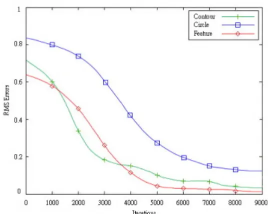
= = − = nTr i nOut j j i j i y t nTr RMSE 1 1 2 , , ) ( 1 (42) where the ntr is the number of training data, nOut is the number of network output, and ti,j and yi,j is the jth target output and real network output of ith training data, respectively. The back-propagation algorithm’s learning curves by three kind of characteristic value fetching methods are show by Fig.10.The performance of the back-propagation network is affected by many factors. If the performance is not good then the recognition rate of our method is also bad. One of the effect factors is hidden node numbers. In Fig.11, we test the back-propagation learning network structure’s hidden node number each and counts impact on recognition rate. Feature-based fetching algorithm has the minimum RMSE of our methods, and we want to know the recognition rate with hidden node number’s effect by feature-based fetching method. So we make the network’s hidden node numbers of feature-based fetching method, for 10 to 15, probe into node number impact on recognition rate respectively from this experiment. In there shows the best recognition rate in network with 10 hidden nodes. We find its recognition rate is up to 90%, so our network structure uses 10 hidden nodes to hidden layer.
Next, we try to find out the three methods of fetching characteristic value, which can be used to reach the better recognition performance. At the same time, we also make other reflectance model’s 3D face database by diffuse [29], specular [30], and cICA [6] reflectance model. We take 50 3D images regard as training data, 50 3D images regard as test data in our 3D database for back-propagation learning algorithm in the three layer feed-forward neural network. For efficiency testing, we take the number 15 characteristic values as training data. The inputs data is classified by the neural network with 10 hidden nodes. The result of recognition rate is showed in Table 1. The best recognition rate of our reflectance model is 90.15%. Furthermore, the recognition rate with used feature-based fetching method is close to the best recognition rate. Among other reflectance model 3D face databases, three recognition rates to fetch method, group different to have different high or low prices each in accordance with reflectance model, but method of us no matter in which characteristic fetching method which recognition rate is most high. It means that the feature-based method is an effective method.
Figure 10. Back-propagation algorithm’s learning curves by three kind of characteristic value fetching
methods.
Figure 11. The back-propagation learning network structure’s hidden node number each and counts
impact on recognition rate.
Table 1. Each reflectance model pick the recognition rate followed the example of three fetching methods on characteristic value.
6. Conclusion
In this paper, we proposed a new reflectance model for 3D surface reconstruction. IKICA as applied in this paper with temporal constraints results in a useful technique for the fast and efficient extraction of surface normal vectors from three surface reflection images. An
important result derived from using the IKICA model for solving photometric stereo problems is that desired output values and smoothing conditions are not needed. This allows for easier convergence and makes the system stable.
For 3D surface reconstruction, several conclusions are listed below. (a) When we estimate the surface shape, the success of the The diffuse reflectance model ([29]) The specular reflectance model ([30]) The cICA reflectance model ([6]) The proposed reflectance model Reflectance model Fetching
method Rate of Recognition (%)
Contour method 62.31 31.36 85.12 88.32
Circle method 59.61 45.02 79.52 82.75
reflectance model depends on two major components, including the diffusion and specular components. (b) In our methods, we do not know the locations of light sources for solving the photometric stereo problems. (c) The proposed IKICA network does not need any special parameter setting and the smoothing conditions.
For 3D face recognition, in order to make the neural network works properly, we need to find the weights and biases by the learning algorithms. In this study, the supervise learning is used. The network is given a set of training data which contains a number of input pattern and corresponding target output. The learning objective is to reach the high accuracy of classification by minimize the error between target output and network output in the training set. Furthermore, the trained classifier also should to provide a good performance in the untrained data.
In the future, we will study other efficient detection algorithms and integrate global characteristic value to further improve the recognition performance of this system. We hope for combining 2D and 3D information of human face in our recognition system effectively to achieve higher recognition rate. Finally, we expect that one day the proposed method could be used to realize a 3D human face recognition system.
Acknowledgements
This work was supported by National Science Council, R.O.C., under grant NSC95-2221-E-390-040-MY2.
Refernce
[1] REFE K. Hayakawa, “Photometric Stereo under a Light Source with Arbitrary Motion,” Journal of the Optical Society of America: A, 1994, Vol. 11, No. 11, pp. 621-639.
[2] G. McGunnigle, “The Classification of Textured Surfaces under Varying
Illuminant Direction,” Ph.D. Thesis, Department of Computing and Electrical Engineering, Heriot-Watt University, Edinburgh, 1998.
[3] C. T. Lin, W. C. Cheng, and S. F. Liang, “A 3-D Surface Reconstruction Approach Based on Postnonlinear ICA Model,” IEEE Transactions On Neural Networks, November, 2005, Vol. 16, No. 6, pp. 1638-1650.
[4] A. Hyvärinen, J. Karhunen, and E. Oja: Independent component analysis, John Wiley & Sons, Inc., 2001.
[5] W. Lu and J. C. Rajapakse, “ICA with reference,” in Proc. 3rd Int. Conf. Independent Component Analysis and Blind Signal Separation: ICA2001, 2001, pp. 120-125.
[6] W. S. Lee, W. C. Cheng, and C. J. Lin, “A cICA-based Photometric Stero for 3D Human Face Reconstruction,” 19th IPPR Conference on Computer Vision, Graphics and Image Processing, 2006, pp. 67-73.
[7] K. R. Muller. S. Mike, G. Ratsch, K. Tsuda, and B. Scholkopf, “An Introduction to Kernel-Based Learning Algorithm,” IEEE Transactions on Neural Network, March, 2001, Vol. 12, No. 2, pp. 181-201.
[8] Kocsor and L. Toth, “Kernel-Based Feature Extraction with a Speech Technology Application,” IEEE Transactions on Signal Processing, August, 2004, Vol. 52, No. 8, pp. 2250-2263.
[9] F. R. Bach, and M. I. Jordan, “Kernel Independent Component Analysis,” IEEE ICASSP, 2003, pp. 876-879.
[10] Xu, X. Jin, and P. Guo, “KICA Feature Extraction in Application to FNN based Image Registration,” International Joint Conference on Neural Networks Sheraton Vancouver Wall Centre Hotel, Vancouver, BC, Canada, July 16-21, 2006, pp. 3602-3608.
[11] G. Y. An, and Q. Ruan “KICA for Face Recognition Based on Kernel Generalized Variance and Multiresolution Analysis,” IEEE
Proceedings of the First International Conference on Innovative Computing, Information and Control, 2006, pp. 3721-3733.
[12] J. Cheng, Q. Liu, and H. Lu, “Texture Classification Using Kernel Independent Component Analysis,” IEEE Proceedings of the 17th International Conference on Pattern Recognition, 2004, pp. 567-578.
[13] T. Martiriggiano, M. Leo, P. Spagnolo, T. D’Orazio, “Facial Feature Extraction by Kernel Independent Component Analysis,” IEEE, 2005, pp. 270-275. [14] R. T. Frankot and R. Chellappa, “A
Method for Enforcing Integrability in Shape From Shading Algorithms,” IEEE Trans. on Pattern Analysis and Machine Intelligence, July, 1988, Vol. 10, No. 4, pp. 439-451.
[15] R. J. Woodham, “Photometric Method for Determining Surface Orientation from Multiple Images,” Journal of Optical Engineering, 1980, Vol. 19, No. 1, pp. 323-367.
[16] P. N. Belhumeur, D. J. Kriegman, and A. L. Yuille, “The Bas-Belief Ambiguity,” CVPR, 1997, pp. 1060-1066.
[17] S. Georghiades, P. N. Belhumeur, and D. J. Kriegman, “From Few to Many: Illumination Cone Models for Face Recognition under Variable Lighting and Pose,” IEEE Trans. on Pattern Analysis and Machine Intelligence, June, 2001, Vol. 23, No. 6, pp. 643-660.
[18] S. Georghiades, “Incorporating the Torrance and Sparrow Model of Reflectance in Uncalibrated Photometric Stereo,” Proceedings of the Ninth IEEE International Conference on Computer Vision, 2003, pp. 352-361.
[19] Z. Zhang, “Image-based modeling of objects and human faces,” Proceedings of SPIE, Video metrics and Optical Methods for 3D Shape Measurement, San Jose, USA, January, 2001, Vol. 4309, pp. 1-15.
[20] F. Pighin, J. Hecker, D. Lischinski, R. Szeliski, D.H. Salesin, “Synthesizing realistic facial expressions from photographs,” SIGGRAPH, 1998, pp. 75-84.
[21] Z. Liu, Z. Zhang, C. Jacobs, M. Cohen, “Rapid modeling of animated faces from video,” Technical Report, Microsoft Corporation, 2000.
[22] B. Nagel, J.Wingbermühle, S.Weik, C.E. Liedtke, “Automated modeling of real human faces for 3D animation,” Proceedings of ICPR, Brisbane, Australia, 1998, pp. 657-676.
[23] R. Koch, “Adaptation of a 3D facial mask to human faces in videophone sequences using model based image analysis,” Picture Coding Symposium, Tokyo, Japan, September, 1991, pp. 285-288.
[24] L. Zhang, “Estimation of eye and mouth corner point positions in a knowledge-based coding system,” SPIE, Digital Compression Technologies and Systems for Video Communications, Berlin, October, 1996, Vol. 2952, pp. 21-28.
[25] G. Gordon, “Face recognition from frontal and profile views,” Proceedings of IWAFGR, Zurich, 1995, pp. 47-52. [26] L. Yin, L. Yin, M. Yourst, “3D face
recognition based on high-resolution 3D face modeling from frontal and profile view,” Proceedings of ACM SIGMM Workshop on Biometrics Methods and Applications, Berkley, California, 2003, pp. 1-8.
[27] R. C. Lacher, S. I. Hruska, and D. C. Kuncicky, “Back-propagation learning in expert networks,” IEEE Trans. on Neural Networks, January, 1992, Vol. 3, No. 1, pp. 62-72.
[28] The Yale Face Database B, Online available
http://cvc.yale.edu/projects/yalefacesB/ yalefacesB.html.
[29] S. Georghiades, P. N. Belhumeur, and D. J. Kriegman, “From few to many: Illumination cone models for face recognition under variable lighting and
pose,” IEEE Trans. on Pattern Analysis and Machine Intelligence, June, 2001, Vol. 23, No. 6, pp. 643-660.
[30] S. Y. Cho and T. W. S. Chow, “Learning parametric specular reflectance model by radial basis function network,” IEEE Trans. on Neural Networks, November, 2000, Vol. 11, No. 6, pp. 1498-1503.
![Figure 7. (a)-(c) Three training images with different light source positions from Yale Face Database B [28] in frontal](https://thumb-ap.123doks.com/thumbv2/9libinfo/8815914.230006/10.892.102.437.641.1059/figure-training-images-different-source-positions-database-frontal.webp)