全光都會環狀骨幹及其光纖/無線擷取網路整合技術---子計畫五：WDM光纖環狀網路資源控制策略設計之研究

行政院國家科學委員會補助專題研究計畫

█ 成 果 報 告

□期中進度報告

具

QoS 保證機制都會光纖網路資源控制策略設計之研究

(The Resource Control Strategy for QoS Guaranteed Optical Metro Mesh/Ring Networks)

計畫類別：□個別型計畫

整合型計畫

計畫編號：

98-2221-E-009-058-MY3

執行期間：98 年 8 月 1 日至 101 年 7 月 31 日

計畫主持人：張仲儒

教授

共同主持人：

計畫參與人員：

陳振宇、葉長青、蔣佩珊、穆瑞、王華立、劉韋成、楊

巧翎、楊明翰、林冠宇、高瑋峻

成果報告類型(依經費核定清單規定繳交)：□精簡報告

完整報告

本成果報告包括以下應繳交之附件：

□赴國外出差或研習心得報告一份

□赴大陸地區出差或研習心得報告一份

□出席國際學術會議心得報告及發表之論文各一份

□國際合作研究計畫國外研究報告書一份

處理方式：除產學合作研究計畫、提升產業技術及人才培育研究計畫、

列管計畫及下列情形者外，得立即公開查詢

□涉及專利或其他智慧財產權，□一年□二年後可公開查詢

執行單位：

國立交通大學電信工程研究所

中 華 民 國 101 年 07 月 05 日

■ 中、英文摘要及關鍵詞(keywords)：（此部分的頁碼編寫請用羅馬字 I 、II、 III…標在 每頁下方中央） ■ 目錄：（此部分的頁碼編寫請用羅馬字I 、II、 III…標在每頁下方中央） ■ 報告內容：（「報告內容」至「附錄」部分請以阿拉伯數字1.2.3.…順序標在每頁下方中 央） ●計畫緣由及目的 ●研究方法 ●結果與討論：含結論與建議 ●參考文獻 ※若該計畫已有論文發表者，可以A4 紙影印，作為成果報告內容或附錄，並請註明發 表刊物名稱、卷期及出版日期。 ※若有與執行本計畫相關之著作、專利、技術報告、或學生畢業論文等，請在參考文獻 內註明之，俾可供進一步查考。 ■ 計畫成果自評：請就研究內容與原計畫相符程度、達成預期目標情況、研究成果之學術 或應用價值、是否適合在學術期刊發表或申請專利、主要發現或其他有關價值等，作一 綜合評估。 ■ 可供推廣之研發成果資料表：凡研究性質屬應用研究及技術發展之計畫，請依國科會提 供之表格，每項研發成果填寫一份。 ■ 附錄（或附件）

國科會補助專題研究計畫成果報告自評表

1. 請就研究內容與原計畫相符程度、達成預期目標情況作一綜合評估

█達成目標

說明：

2. 研究成果在學術期刊發表或申請專利等情形：

論文：█已發表 □未發表之文稿 □撰寫中 □無

專利：□已獲得 □申請中 □無

技轉：□已技轉 □洽談中 □無

其他：（以

100 字為限）

3. 請依學術成就、技術創新、社會影響等方面，評估研究成果之學術或應用價

值（簡要敘述成果所代表之意義、價值、影響或進一步發展之可能性）（以

500 字為限）

計畫中文摘要

高速都會區域網路中的彈性分封環(Resilient Packet Ring)中訊務控制所需考 慮的議題主要希望可以達到公平性的頻寬分配並且可以快速穩定各訊務流。我們 提出一個高效能乏晰公平流速產生器(fuzzy local fairRate generator, FLAG)，藉著 乏晰運作機制產生一個準確的本地公平流速來抑制壅塞情況並且達成上述考 量。所提出的機制，是由三個部份所組成，適應性公平流速計算器(adaptive fairRate calculator, AFC)、乏晰壅塞偵測器(fuzzy congestion detector, FCD)、與乏 晰公平流速計算器(fuzzy fairRate generator, FFG)。適應性公平流速計算器產生一 個評估過的公平流速而乏晰壅塞偵測器根據次級傳輸緩衝器(STQ)的容納量與接 收到的流量大小來指出當前的壅塞程度。乏晰公平流速計算器經由考量兩項由適 應性公平流速計算器與乏晰壅塞偵測器輸出的結果來得到反映真實流量狀況的 本地公平流速。藉由適應性公平流速計算器與乏晰壅塞偵測器的使用，乏晰公平 流速產生器可產生較小的收斂時間，再者當與其它演算法相比，在不同大小的壅 塞區域中皆獲得極好的效果。 基於頻寬的需求，以及服務更廣大的區域，多個彈性分封環可橋接成一個 跨環式彈性分封環網路BRPR(Bridged RPR)。但是該橋接式網路第一個需要考慮 的就是路由控制問題。在此環境中，我們基於載量均衡原則(the load balancing principle)提出一個智慧型跨環路由控制法。該智慧型跨環路由控制法不只同時考 慮橋接器以及下游擷點雍塞的情況並且同時考量橋接器的服務速率以及訊務終 點站與橋接器的距離。

此外，在光叢集交換(Optical Burst Switching)環中，頻寬利用率、公平性、 和穩定性都是很重要的議題。我們提出了一個波長分配與訊務控制(WATC)的方 案來達成上述的考量。系統採用了預約的機制來避免時槽式系統中資料的碰撞， 而且為了減少光電之間的轉換，每個節點中都沒有過境緩衝器。首先，排程器會 依據入口緩衝器中佇列的權重來分配頻寬，然後由波長分配器(WA)決定適合的 位置。波長分配器會適時地調整將要產生的資料叢集的大小，藉此有效利用空隙 並提升頻寬利用率。另一方面，為了減輕一個下游節點可能遭受到頻寬挨餓的問 題，一個乏晰保護性預約產生器(FPRG)會參考過境訊務的情況，動態地預留一 些頻寬給入境的聲音與影像訊務。然後，公平流速產生器(FRG)再根據剩餘的頻 寬產生一個評估過的公平流速，並由訊務控制器(TC)決定出最終宣傳的公平流速 來規範上游的節點。 關鍵詞：彈性分封環、跨環式彈性分封環網路、公平性、服務品質、光叢集交換 環、波長分配、訊務控制

Abstract

The resilient packet ring (RPR) is a ring based network for high-speed metropolitan area networks which has properties of fault tolerance and high bandwidth utilization. In RPR, the issues of fairness, stability, and convergence timeare important in congestion control. A local fairRate generator using fuzzy logic and the moving average technique is proposed for the RPR. The fuzzy local fairRate generator (FLAG) is designed to achieve both low convergence time and high system throughput, besides fairness. It contains three functional blocks, an adaptive fairRate calculator (AFC) to properly preproduce a local fairRate by the moving average technique, a fuzzy congestion detector (FCD) to intelligently estimate the congestion degree of the station, and a fuzzy fairRate generator (FFG) to precisely generate the local fairRate. Simulation results show that only the FLAG can stabilize all flows inparking lot scenarios with different finite traffic demands, compared with the conventional aggressive mode (AM) and distributed bandwidth allocation (DBA) fairness algorithms.

Also, we propose an intelligent inter-ring route control, employed in the bridges which connect two RPRs, for the BRPR. The intelligent interring route controller (IIRC) is designed according to the load balancing principle, where the IIRC considers not only the congestion degree of both bridge and its downstream nodes but also the service rate and the number of hops to destination. Simulation results show that the IIRC improves the performances in the packet dropping probability, the average packet delay, and the throughput over the queue length threshold route controller (QTRC) and the shortest path route controller (SPRC).

Finally, the optical burst switching (OBS) ring network is mainly designed for high-speed metropolitan area network, which is expected to support many kinds of services. In the OBS rings, the issues of bandwidth utilization, service differentiation, fairness, and stability are important. A wavelength assignment and traffic control (WATC) scheme is proposed to achieve these considerations. The reservation mechanism is adopted to avoid burst collisions in the time-slot based system, and no transit buffers are deployed at each node for the reason of bypassing the traffic directly. The wavelength assigner (WA) cooperates with the scheduler to generate and then transmit data at the determined position, thereby increasing the bandwidth utilization and supporting service differentiation. In order to alleviate the bandwidth starvation problem a downstream node may suffer from, a fuzzy protective reservation generator (FPRG) preserves some bandwidth for ingress voice and video traffic referring to the network conditions. Afterwards, the fair rate generator (FRG) produces an estimated fair rate, and the traffic controller (TC) determines the advertised fair rate which regulates the upstream node. Since the observation window

is applied, the convergence time is reduced.

Keywords： Resilient packet ring, Bridged resilient packet ring, Fairness, Optical burst switching ring, Wavelength assignment, Traffic control

Agenda

I. Introduction...1

II. FLAG: A Fuzzy Local FairRate Generator for Resilient Packet Ring ...6

III. Intelligent Inter-Ring Route Control in Bridged Resilient Packet Rings ………....11 IV. Reservation Slotted OBS Rings with Wavelength Assignment and Traffic

Control ...23

V. Reference... 35 VI. Comment ...38

I. Introduction and Motivation

In development of the Internet, the technology of the wavelength division multiplexing (WDM) has impacted the designment and realization of the next gerneration network. From the piont-to-point transport technology, the next generation network can be mainly divided into two types: long haul backbone (core) network and the metropolitan area networks (MAN). For the first network type, long haul backbone (core) network, the main challenge is how to keep data in the optical domain as much as possible. For the second network type, how to support the QoS, allocate bandwidth based on fairness, and avoid or solve congestion are the main problems.

Several approaches have proposed to take advantage of optical communication to develop the long haul backbone (core) network. Three of these approaches are the Optical Circuit Switching (OCS), the Optical Packet Switching (OPS), and the Optical Burst Switching (OBS) [1]-[6]. The main attraction of optical switching is that it should enable routing of optical data signals without the need for conversion to electrical signals and, therefore, should be independent of data rate and data protocol. Also, the three optical switchings could promise for the gradual migration of the switching functions from electronics to optics. While OCS provides bandwidth at a granularity of a wavelength, OPS can offer an almost arbitrary fine granularity, comparable to currently applied electrical packet switching, and OBS lies between them.

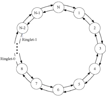
The ring network with the natural advantage, such as simple archtechure, easily adding or removing nodes, the fault tolerance property, and the needless routing property, is the prevalent topology used in metropolitan area networks (MANs). The resilient packet ring (RPR) is a dual-ring-based optical packet network, as shown in Fig. 1.1, and has been recently approved as the IEEE 802.17 Standard [7]. The resilient packet ring (RPR) is constructed by several pairs of two unidirectional links between stations. The RPR can provide guaranteed quality of service parameters and support service monitoring including performance management and fault management [7, 8]. Besides, the RPR has some noticeable properties such as spatial reuse, fair bandwidth allocation, and fast network failure recovery to get rid of deficiencies of conventional high-speed Ethernet and SONET [9, 10]. Therefore, the RPR can not only achieve high bandwidth utilization and fast network failure recovery but also satisfy the requirements of MANs, such as reliability, flexibility, scalability, and large capacity [9, 10, 11]. The RPR is a superior candidate for MANs.

Figure 1.1: RPR structure

The spatial reuse allows a frame to be removed from the ring at its destination so that the bandwidth on next links can be re-used at the same time. Also, the fair bandwidth allocation avoids stations at upstream transmitting too many lowpriority frames to cause stations at downstream system congestion. RPR needs congestion control to enhance the fair bandwidth division in the congestion domain which is defined in the IEEE 802.17 [9, 12]. The congestion control implemented in each station should periodically generate an advertised fairRate to advertise its upstream station for regulating the added fairness eligible (FE) traffic flow defined in IEEE 802.17 [9, 12]. The advertised fairRate should be determined referring to the local fairRate, the received fairRate, and the congestion degree of the station. The local fairRate is generated by a fairness algorithm, and the received fairRate is the advertised fairRate from the downstream station.

Two key factors affect performance of the fair bandwidth allocation: congestion detection and fairness algorithm. If the congestion detection is too rough, it would lower the networks throughput or raise frame loss. The fairness algorithm should consider the most important performance issues of FE traffic flows: stability, fairness, convergence time, and throughput loss caused by the FE traffic flow oscillation. The stability would avoid the oscillation of regulated FE traffic flows, which would cause the throughput loss. If a fairness algorithm referees a ring ingress aggregated with spatial reuse (RIAS) fairness, it has been proved that the algorithm will achieve high system utilization [13]. It is because the RIAS has two key properties.

The first property is that an ingress-aggregated (IA) flow fairly shares the bandwidth on each link, relating to other IA flows on the same link, where an IA flow

is the aggregate of all flows originating from a given ingress station. The second property is that the maximal spatial reuse subjecting to the first property. Thus, the bandwidth can be reclaimed by IA flows when it is unused. In summary, the RIAS is a max-min fairness with traffic granularity of IA flow. The convergence time is the time interval between the instant of starting the congestion occurrence and the instant that the amount of arriving specified traffic flow approaches the ideal fairRate which meets the the RIAS fairness. Therefore, a fairness algorithm should achieve not only high stability based on the RIAS fairness but also low convergence time and flow oscillation. There are two conservative modes (CM) [9, 13] and the aggressive mode (AM) [9, 10] fairness algorithms, which have been proposed in IEEE 802.17. Actually, the AM fairness algorithm performs better than the CM fairness algorithm. Unfortunately, the AM suffers from severe oscillations and bandwidth utilization degradation [9, 12]. It is due to the fact that the AM issues an un-limited fairRate, called FullRate, as its advertised fairRate when the station is released from congestion.

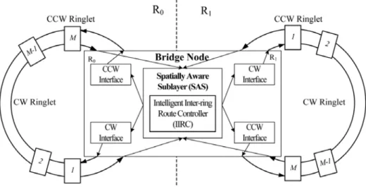
Multiple RPR rings can be bridged together to form a larger network, named bridged-RPR network (BRPR), by a bridge which forwards packets from one RPR to another RPR, shown in Fig.1.2. A spatially aware sublayer (SAS), which is a part of the MAC layer, in the bridge is used to decide which ringlet interface the packet should be routed to [7, 14]. Current research on SAS, including the IEEE 802.17b Working Group, is mainly focusing on how to modify this sublayer in order to avoid flooding the entire bridged network when transmitting inter-ring packets [7, 14, 15, 16].

Figure 1.2: BRPR structure

OBS ring topologies have been a good choice for solving the current metro gap problem between core network and access network owing to its simplicity and scalability.

I.1. FLAG: A Fuzzy Local FairRate Generator for Resilient Packet Ring

Since the Resilient Packet Ring (RPR), unlike legacy technologies, supports destination packet removal so that a packet will not traverse all ring nodes and spatial reuse can be achieved. However, allowing spatial reuse introduces a challenge to ensure fairness among different nodes competing for ring bandwidth [13]. The RPR defines two fairness algorithms, conservative mode (CM) [9, 13] and the aggressive mode (AM) [9, 10] fairness algorithms, that specify how upstream traffic should be throttled according to downstream measurements, named an advertised fairRate.

The upstream nodes would appropriately configure their rate limiters to throttle the rate of injected traffic to its fair rate. Unfortunately, both the two RPR fairness algorithms have a number of important performance limitations. First, they are prone to severe and permanent oscillations in the range of the entire link bandwidth in simple unbalanced traffic network environment, in which all flows do not demand the same bandwidth. Second, they could not fully achieve spatial reuse and fairness. Third, they must take much time to stabilize all flows [13, 17]. The operations of the two algorithms are described as follows.

In AM, the congested station also calculates and advertises a fairRate estimate periodically without waiting to evaluate the received traffic which is regulated by the previously transmitted advertised fairRate. Also, the calculation of the fairRate is based solely on preset parameters and the station’s added rate which is the traffic added in ringlet. The frequent advertisement of new fairRate brings a more ”aggressive” algorithm, thus more quickly attempts to adapt to changing traffic conditions.

However, the faster response as compared to the conservative mode induces the risk of instabilities that flows oscillate permanently, when rate adjustments are made faster than the system is able to respond. In CM, the congested station transmits an advertised fair rate to upstream, and then waits to see the change in traffic from upstream stations. If the observed effect is not the fair division of rates, then the congested station calculates a new fair rate estimate again, and distributes it to upstream.

Several fairness algorithms were proposed to solve this problem and some of them were designed based on the RIAS fairness [13, 17-22]. The distributed virtualtime scheduling (DVSR) [13] is proposed by Gambiroza et al. and it mainly

computes a simple lower bound of temporally and spatially aggregated virtual time using per-ingress counter of packet arrival. The aggregated information propagates along the ring to let each station know the traffic condition of downstream stations. Therefore, each node is capable of limiting its output rate to satisfy RIAS fairness.

Unfortunately, it is at the expense of a high computational complexity O(NlogN), where N is the number of stations in the ring. Alharbi and Ansari proposed a distributed bandwidth allocation (DBA) fairness algorithm with a low computational complexity O(1) [17, 18]. The DBA measures the arrival rate so as to calculate the effective number of ingress-aggregated (IA) flows, where IA flow represents the aggregate of all flows originating from a given ingress station, transiting over the local station. By a recursive method, DBA uses the effective number of IA flows and the remaining bandwidth to obtain the advertised fairRate. After some rounds of recursion, an advertised fairRate which satisfies RIAS fairness can be obtained. However, whenever the effect of propagation delay is severe, the DBA would not be a stable local fairRate algorithm. It is because the local fairRate generated by DBA is related only with the amount of the arriving transit FE traffic flows measured during a short frame time. This shortterm amount is easily influenced by the effect of the propagation delay, which starts from a station sending its advertised fairRate and ends the corresponding transit traffic flows arriving the station. If the propagation delay is large, the short-term arriving transit FE traffic flows would be largely varied and make the generation of local fairRate unstable (incorrect).

Moreover, Yilmaz and Ansari investigated weighted fairness in IEEE802.17 but found one unexpected phenomenon [20]. When a station with a larger weight becomes a head of congestion domain, it leads to an undesirable result of bandwidth allocation and oscillation. However, after modifying a little in original fairness algorithm of AM, it can work correctly under weighted fairness.

I.2. Intelligent Inter-Ring Route Control in Bridged Resilient Packet Rings

Settawong and Tanterdtid proposed an enhancement by using a topology discovery and spanning tree algorithm [15]. The algorithm can manage traffic between rings more efficiently and can remove the need for flooding. The shortest path route controller (SPRC) was widely considered for metro rings [23, 24, 25] as it can maximize the spatial reuse and thus the achievable packet throughput for uniform traffic.

However, as traffic load increases, incoming call requests could pile up at a node before being processed, and these would result in a potential bottleneck in network

performance [25]. Also, Heiden et. al. analyzed the capacity of bidirectional optical packet ring networks, such as RPR, which employs the SPRC for multicast hotspot traffic [26]. They found that when the multicast traffic originating at the hotspot exceeds a critical threshold, the SPRC leads to a significant capacity reduction.

Intuitively, the route selection would be closely related with the congestion degree of the ringlet so as to follow the load balancing principle. Generally, RPR uses a queue length threshold to detect the congestion and a nodes adding rate limitation to avoid the network congestion [7]. Therefore, an intuitive queue-length threshold route controller (QTRC) would be better than the SPRC. However, the correlation function between the congestion degree and these variables is nonlinear and complicated.

I.3. Reservation Slotted OBS Rings with Wavelength Assignment and Traffic Control

Each network node in an OBS ring network employs transmitters and receivers to send and receive data traffic. There are several architectures with variants combinations of transmitters and receivers in OBS nodes [27, 28, 29]. A more scalable and flexible system with tunable transmitter–tunable receiver (TT–TR) architecture was also proposed [27]. Its advantages come at the expense of a higher resource contention possibility and a higher packet loss probability. In this paper, we adopt the TT-TR architecture for the reason of scalability.

At each node, packets with the same destination are assembled into a data burst (DB) by assembly algorithm, such as length based algorithm, time based algorithm and hybrid algorithm [30]. The DB must be transmitted according to a specific medium access control (MAC) protocol to avoid burst collisions. Several proposed MAC protocols can be classified into two major categories: token based scheme [31, 32] and time-slot based scheme [33]. Unfortunately, the token based schemes cause low channel utilization. The time-slot based scheme solves this problem, but it does not assure class of service (CoS).

Wavelength assignment is an important work in OBS networks. An appropriate wavelength assignment method not only makes better use of link bandwidth but also supports CoS. Some methods of wavelength assignment have been proposed for OBS network [34, 35, 36]. For ring networks, however, there is still a problem of bandwidth sharing among the nodes. When traffic load increases, the downstream nodes may suffer from bandwidth starvation. A traffic control method can prevent this situation and provide fair access to the link bandwidth. There are some methods of traffic control proposed for resilient packet ring (RPR) which is also a ring based network [37, 38].

II. FLAG: A Fuzzy Local FairRate Generator for Resilient Packet Ring

 Architecture of Intermediate OBS Node

Assume that a resilient packet ring (RPR) with N stations, shown in Fig. 1.1, is constructed by two unidirectional, counter-rotating ringlets, named ringlet-0 and ringlet-1. Each station has two pairs of input and output ports to communicate with neighbor stations. Station X (Y) is said to be a upstream (downstream) node of station Y (X) on ringlet-0 or ringlet-1 if the station Y (X) traffic becomes the received traffic of station X (Y) on the referenced ringlet. There are three classes of service for RPR. The classA is used for real-time services and it has subclassA0 for reserved bandwidth and subclassA1 for reclaimable bandwidth. The classB is targeted for near real-time services, and it also has two subclasses: classB-CIR (committed information rate) which requires the bounded delay and guaranteed bandwidth, and classB-EIR (excess information rate) which does not guarantee bandwidth or delay bound. The classC is intended for best effort services and has the lowest priority. Each station only reserves bandwidth for subclassA0, and the remaining bandwidth is provided for other traffic classes according to the order of subclassA1, classB-CIR, classB-EIR, and classC. The latter two low priority traffics are called the fairness eligible (FE) traffic and are controlled by a fairness algorithm.

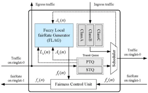
Fig. 2.1 shows the station structure for ringlet-0 transmisson, which contains an ingress queue with ClassA, ClassB, and ClassC queues, a transit queue with primary transit queue (PTQ) and secondary transit queue (STQ), a scheduler, the fuzzy local fairRate generator (FLAG), and a fairness control unit. The ClassX queue, X = A, B, or C, stores the added classX traffic to the station. The PTQ (STQ) stores the transiting classA and classB-CIR (classB-EIR and classC) frames. The scheduler decides the transmitting order. If the STQ occupancy is less than the stqHighthreshold defined in the IEEE802.17 [17], the order is PTQ, ClassA, ClassB, ClassC, and STQ; otherwise, it is PTQ, ClassA, ClassB, STQ, and ClassC. The FLAG generates a local fairRate at every time nT, denoted by fl(n), where n is a positive integer and T is the duration of an agingInterval. Notice that fl is also generated per agingInterval in DBA but is generated only when the station is in congestion in AM. The fairness control unit usually refers to both fl(n) and the received fairRate, denoted by fr(n), to determine an advertised fairRate, denoted by fv(n), and then sends fv(n) to upstream stations to regulate traffic flows, at every agingInterval time nT.

Figure 2.1: RPR station structure

The advertised fairRate generated by the fairness control unit are described as follows. The fv would be set to be fl if fr is smaller than fl and larger than the bandwidth rate of the transit FE traffic flows which will pass through the originally congested station. Otherwise, it is set to be min(fl, fr). Here we also describe the advertised fairRate generated by AM below. When the station is congestion free, the fv is set to be the FullRate if the fr is larger than the bandwidth rate of the transit FE traffic flows which will pass through the originally congested station; to be fr, otherwise. The FullRate is a specially advertised fairRate to indicate that the station does not need to limit its added FE traffic flow. When the station is in congestion, the

fv is set to be fl if the fr is FullRate; to be min(fl, fr), otherwise. Note that the

congestion is occurred at a station for AM if the STQ occupancy of the station is larger than the stqLowthreshold, defined in IEEE802.17. Also, the originally congested station is known to the observation station since the message of the advertised fairRate contains a field to record it; the fl is the added FE traffic flow rate to the network.

 Fuzzy Local FairRate Generator (FLAG)

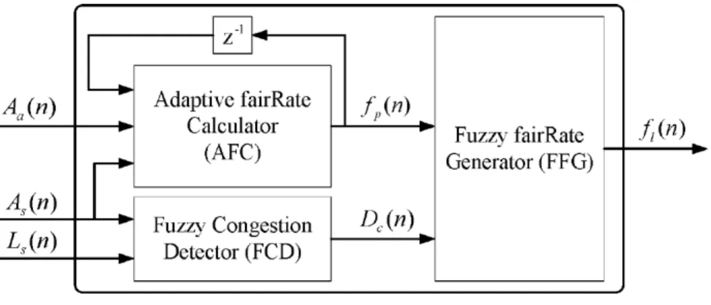
The proposed fuzzy local fairRate generator (FLAG), shown in Fig. 2.2, is composed of an adaptive fairRate calculator (AFC), a fuzzy congestion detection (FCD), and a fuzzy fairRate generator (FFG). During the nth agingInterval which is from time (n − 1)T to time nT, the FLAG determines fl(n) by referring to the arriving FE traffic flows to STQ, denoted as As(n), the added FE traffic flow to the network, denoted as Aa(n), and STQ occupancy, denoted as Ls(n). The AFC pre-generates a local fairRate, called p-fairRate and denoted by fp(n), which satisfies the RIAS

fairness. Its design imitates the DBA’s generation of local fairRate, but it would overcome the unstable (incorrect) local fairRate generation by DBA when the propagation delay is significant. Instead of using the short-term arriving transit FE traffic flows, it calculates a proper average of the arriving transit FE traffic flows by moving average technique to mitigate the effect of the propagation delay. The FCD appraises the congestion status of station using fuzzy logics. Its design can softly detect the congestion degree of the station in each agingInterval n, denoted by Dc(n), considering not only the STQ occupancy but also the amount of the arriving transit FE traffic flows at the queue. The latter term denotes the change rate of the STQ occupancy which would play an important role in the congestion detection. Finally, the FFG generates a precise local fairRate by fine-tuning the p-fairRate from AFC, referring to the congestion degree from FCD, and further using domain knowledge designed by fuzzy logics. The FLAG would avoid serious regulating FE traffic flows to decrease the throughput or excessive relaxing the traffic flows to increase the frame losses..

Figure 2.2: Functional blocks of FLAG  Adaptive fairRate Calculator (AFC)

The adaptive fairRate calculator (AFC) adopts the moving average technique [14] on the short-term arriving FE traffic flows, trying to mitigate the effect of propagation delay on the generation of local fairRate by the DBA [5]. During the n-th agingInterval, the AFC first takes the moving average of arriving transit FE traffic flows to STQ, As(n). Denote the average by ( )

~ n A_s and give it by ~ 1 ( ) n ( ) / s _s i n k A n A n k    



where k is the size of observation window. The k is the sum of two kinds of the data frame trip time: one is the time from the furthest source to this observation station, and the other is the time from this station to originally congested station. It is because the FE traffic flow of a station in this interval would be regulated by an advertised fairRate which is sent out from one of the stations in the interval. The A~_s(n) will not vary too much and become more stable.

Then the AFC computes the effective number of IA flows during the n-th agingInterval, denoted by M (n), which is obtained by

~ ( ) ( ) ( ) ( 1) s _a p A n A n M n f n    . (2.2)

The AFC fairly allocates the remaining bandwidth to these effective IA flows, which would be C(A_s(n)A_a(n)) M . Finally, the AFC calculates the fp(n) by adding up the previous p-fairRate, fp(n-1), and the fairly shared bandwidth. The fp(n) is given by









 Fuzzy Congestion Detector (FCD)

The FCD refers not only the occupancy of STQ, Ls(n), as defined in the IEEE802.17, but also the arriving FE traffic flows to STQ, As(n), to determine the congestion degree, As(n). The As(n) can be viewed as the change rate of STQ, which is also an important variable in the detection of congestion degree

Dc(n). We define the term set for Ls(n) as T(Ls(n)) = {Short (S), Long (L)}; for

As(n) as T(As(n)) = {low (L), Medium (M ), High (H )}; for As(n) as T(As(n)) = {Very Low (VL), Low (L), Medium (M ), High (H ), Very High (VH )}.

Here, the triangular function f









g are used to define the membership functions for the terms in the term set. These two functions are

0 0 0 0 0 0 0 0 1 0 0 1 1 1, for , ( ; , , ) 1, for , 0, otherwise. x x x a x x a x x f x x a a x x x a a   _{   }     _         _(2.4) and 0 0 0 0 0 0 1 0 1 0 1 1 1 1 1 1 1, for , 1, for , ( ; , , , ) 1, for , 0, otherwise x x x a x x a x x x g x x x a a x x x x x a a   _{   }        _  _{   }    _(2.5)

where x0 in f

 

 

The corresponding membership functions of S and L in T (Ls(n)) are denoted by _s(L_s(n))g(L_s(n);0,0.125Q ,0,0.25Q) and ) 0 , 0.25 , 0.35 ); ( ( )) ( (L_s n g L_s n Q, Q Q L 

 , where Q is the size of STQ. As defined in IEEE 802.17 standard, we take 0.125 of the STQ size as the stqLowthreshold to judge the light congestion degree, and 0.25 of the STQ size as the stqHighthreshold to judge the heavy congestion degree. The corresponding membership functions of L, M , and H in T (As(n)) are denoted by )_L(A_s(n))g(A_s(n);0,0.125C,0,0.375C , ) 0.25C 0.25C, 0.5C, ); ( ( )) ( (A_s n f A_s n M   , and ) C 0.375C, C, 0.875C, ); ( ( )) ( (A_s n g A_s n H 

 , respectively. For the reason of simplicity in computation of defuzzification, the corresponding membership functions of VL; L; M ; H; and VH in T (Dc(n)) are defined as

) 0 0, 0, ); ( ( )) ( (D_c n f D_c n VL   , )_L(D_c(n)) f(D_c(n);0.25,0,0 , ) 0 0, 0.5, ); ( ( )) ( (D_c n f D_c n M   , )_H(D_c(n)) f(D_c(n);0.75,0,0 , and_VH(D_c(n)) f(D_c(n);1,0,0), respectively.

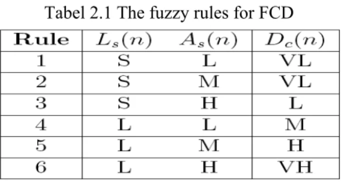
There are 6 fuzzy rules for FCD. As shown in Table 2.1, the order of significance of the input linguistic variables is Ls(n) then As(n). The station with high occupancy of STQ would be in high congestion degree, and it would be in higher (medium) congestion degree if the arriving FE traffic flows to

STQ is also high (low).

Tabel 2.1 The fuzzy rules for FCD

The fuzzy congestion detector adopts the max-min inference method for inference engine because it is suitable for real-time operation. To explain max-min inference method, we take rule 1and rule 2, which have the same control action ” Dc(n) is VL”, as an example. Applying the ”min” operator, we obtain the membership function values of the control action ” Dc(n) is VL” of rule 1 and rule 2, denoted by m1(n) and m2(n), respectively, by

1( ) min{ ( ( )), ( ( ))}S s L s

m n 





2( ) min{ ( ( )), ( ( ))}S s M s

m n 





Subsequently, applying the ”max” operator yields the overall membership function value of the control action ” Dc(n) is VL”, denoted byVL(n), by

1 2

( ) max{ ( ), ( )}

VL n m n m n



The fuzzy inference results of the output indication L, M , H , and VH , denoted by _L(n), _M(n) , _H(n), and _VH(n) , respectively, can be obtained by the same way. Finally, the fuzzy inference results are to be defuzzified to become usable values. The defuzzification method adopted is the center of area defuzzification method, and a crisp value of the congestion degree Dc(n), denoted by z0, can obtained by

0 0.0 ( ) 0.25 ( ) 0.5 ( ) 0.75 ( ) 1.0 ( ) ( ) ( ) ( ) ( ) ( ) VL L M H VH VL L M H VH n n n n n z n n n n n





















The FFG refers the p-fairRate, fp(n), and the congestion degree, Dc(n), as the input variables to generate a proper and robust local fairRate, fl(n) The local fairRate fl(n) affects both the fairness performance and the bandwidth

utilization. Define the term set with six terms for fp(n) as T(fp(n)) = {Extremely Low (EL), Pretty Low (PL), Slightly Low (SL), Slightly High (SH ), Pretty High (PH ), Extremely High (EH )}; the term set with three terms for Dc(n) as T(Dc(n)) ={Low (L), Medium (M ), High (H )}; and the term set with eleven terms for fl(n) as T(fl(n)) ={Extremely Low (EL), Very Low (V L), Pretty Low (PL), Low (L), Slightly Low (SL), Medium (M ), Slightly High (SH ), High (H ), Pretty High (P H ), Very High (V H ), Extremely High (EH )}. Note that the number of the terms in T(fl(n)) would be larger than that of T(fp(n)) for better performance. The membership functions for terms EL; P L; SL; SH; P H; and EH in T(fl(n)) are defined as

) 0.3C 0, 0, ); ( ( )) ( (f_p n f f_p n EL   , ) 0.2C 0.2C, 0.2C, ); ( ( )) ( (f_p n f f_p n PL   , ) 0.2C 0.2C, 0.4C, ); ( ( )) ( (f_p n f f_p n SL   , ) 0.2C 0.2C, 0.6C, ); ( ( )) ( (f_p n f f_p n SH   , ) 0.2C 0.2C, 0.8C, ); ( ( )) ( (f_p n f f_p n PH   , and ) 0 0.3C, C, ); ( ( )) ( (f_p n f f_p n EH 

 , respectively. The membership functions for terms L; M; and H in T(Dc(n)) are defined as

) .375 0 0, 0.125, 0, ); ( ( )) ( (D_c n g D_c n L   , ) 0.25 0.25, 0.5, ); ( ( )) ( (D_c n f D_c n M   , and ) 0 .375, 0 1, 0.875, ); ( ( )) ( (D_c n g D_c n H 

 , respectively. The membership functions for terms in T(fl(n)) are defined as fuzzy singletons, denoted by

) 0 0, , x ); ( ( )) ( ( _{l l T} T f n  f f n  , where T = EL;V L; PL; L; SL; M; SH; H; PH; V H; or EH , and (xEL, xVL, xPL, xL, xSL, xM, xSH, xH xPH xVH xEH) = (0, 0.1C, 0.2C, 0.3C, 0.4C, 0.5C, 0.6C, 0.7C, 0.8C, 0.9C, C). Notice that the center value of the triangular membership function f of each term for fp(n) is the same as the center value of the singleton function f of the same term for fl(n), where these terms are EL; P L; SL; SH; P H; and EH .

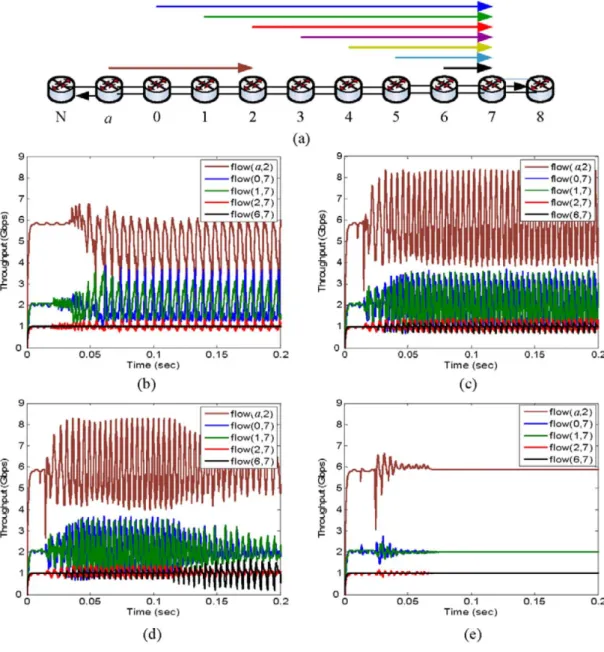
There are 18 fuzzy rules for FFG. As shown in Table 2.2, the order of significance of the input linguistic variables is fp(n) then Dc(n). These fuzzy rules are set in such a way that the generation of fl(n) mainly refers to fp(n) but slightly adjusted by Dc(n) so as to achieve lower convergence time and thus higher the throughput. When fp(n) is ‘’EL’’ or “PL”, fl(n) is designed to raise

two levels more than fp(n) (ELPL or PL  SL) if Dc(n) is “L” and fl(n) remains unchanged if Dc(n) is “H”. This intends to increase the throughput. When fp(n) is “SL”; “SH”; or “PH”, fl(n) decreases one level less than fp(n) if

Dc(n) is “H” and fl(n) increases one level larger than fp(n) if Dc(n) is “L” . When fp(n) is “EH”, fl(n) should be decreased two levels less than fp(n) (EH  PH ) if Dc(n) is “H” and fl(n) remains unchanged if Dc(n) is “L”. This intends to achieve RIAS fairness. Finally, the defuzzifier uses the min-max method to generate a crisp-valued local fairRate.

Tabel 2.2 Rule Base for FFG

 Simulation Result

In the simulations, settings for the environment include 10 Gbps link capacity, 200μs propagation delay between stations, 4 Mbytes STQ size, and 100 μs agingInterval. The value of the stqHighthreshold is 1 Mbytes and the value of the stqLowthreshold is 0.5 Mbytes. Simulations for the proposed FLAG, DBA with moving average technique (DMA), DBA, and AM also conducted for performance comparison. Simulation results are recorded per agingInterval. Also, assume that the reserved bandwidth is zero, and only fairness eligible (FE) traffic flow is considered.

Fig. 2.3(a) shows a small parking lot scenario where there are 5 (0 ∼ 4) greedy stations, and Figs. 2.3(b), 2.3(c), 2.3(d) and 2.3(e) present the throughput of each flow by AM, DBA, DMA, and FLAG, respectively. This small parking lot scenario assumes that flows are generated from station 0, 1, 2, and 3 but terminated atstation 4. The propagation delay is small. It can be seen that FE flows of AM, DBA,

DMA, and FLAG take 49ms, 14ms, 13.5ms, and 7ms to stabilize, respectively. ThusFLAG improves by 7 times over AM and by 2 times over DBA, in the convergence time of traffic flows. The reasons are given as follows. The fuzzy logics provides a robust mathematical method to solve problems which are complicated to find a proper mathematical model for them. Especially, the FLAG contains sophisticated functional blocks, which combine advantages of AM and DBA. It fine-tunes the so-called p-fairRate generated by AFC, according to the congestion degree softly determined by the FCD using the fuzzy logic and the effective fuzzy

rules designed in FFG by expert’s domain knowledge. On the other hand, the DBA and DMA generate the local fairRate depending only on the short-term (average) arriving FE traffic flow, or equivalently the change rate of the STQ, without considering the STQ occupancy which usually used to determine the congestion degree of station. This would incorrectly limit the amount of the passing transit FE traffic flow to the next station and cause DBA make error decision. For example, if the amount of the short-term arriving transit FE traffic flow is large but the STQ occupancy of a station is short, the station should not seriously regulate the FE traffic flow of its upstream stations. Also, AM generates a local fairRate which is equal to the added FE traffic flow rate of the station to regulate the flow when the station is in congestion. AM immediately sets the advertised fairRate as FullRate to allow the upstream stations to un-limitedly send traffic flow when the congestion is released. This too-much variation of the advertised fairRate would cause the station congestion again and thus make the flow of AM damping the longest.

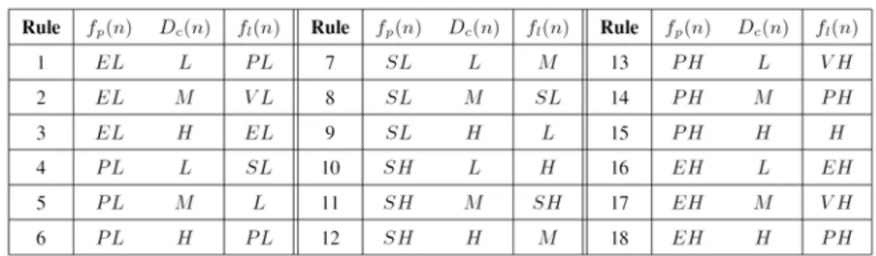
Figure 2.3: (a) Small parking lot scenario with greedy traffic, and the throughput of (b) AM, (c) DBA, (d) DBA with moving average (DMA), and (e) FLAG. Fig. 2.4(a) shows a large parking lot scenario where there are containing 8(0 ∼ 7)

greedy stations, and Figs. 2.4(b), 2.4(c), 2.4(d) and 2.4(e) presentthe throughput of flow(0, 7), flow(2, 7), flow(4, 7), and flow(6 ,7) at station 7 by AM, DBA, DMA, and FLAG, respectively. This scenario differs from the previous one of Fig. 2.3 in that the propagation delay would be large. It can be seen that the FLAG and the AM take 11ms and 27ms to stabilize the flows, respectively; unfortunately, DBA and DMA take quite a long time to stabilize the traffic flows.

It is because that DBA computes the number of the effective IA flows referring to both the short aggregating traffic (per agingInterval) and the pervious local fairRate to generate the current local fairRate. However, due to the large propagation delay, the correlation between the short aggregating traffic and the pervious local fairRate becomes low. Therefore, DBA cannot generate a correct local fairRate to regulate flows. Thus the flows oscillate and converge slowly; the convergence time takes about 0.15s which is not shown here. The DMA uses the moving average technique to lessen the effect of propagation delay. The flow oscillation of the DMA is half smaller than the DBA but still exists. Since without considering the STQ occupancy for the congestion degree of station, the DMA incorrectly limits the amount of the passing transit FE traffic flow to the next station. On the other hand, the FLAG can correctly generate the p-fairRate to meet the RIAS fairness and diminish the effect of the propagation delay to some extent. Also, the FLAG finely adjusts the p-fairRate to a precise local fairRate according to both the congestion degree and the effective fuzzy rules well designed by domain knowledge. The main reason that AM in this scenario takes less time to stabilize all flows than AM in the previous scenario shown in Fig. 2.3(b) is given below. Since, here in Fig. 2.4(a), there are more stations with greedy traffic, more aggregated traffic per agingInterval will be caused. This more aggregated traffic and the larger propagation delay would make the station congestion always occur earlier. Afterwards, the station would not have the chance to set the advertised fairRate as FullRate. Thus the convergence time is shorter.

Figure 2.4: (a) Large parking lot scenario with greedy traffic, and the throughput of (b) AM, (c) DBA, (d) DMA, and (e) FLAG.

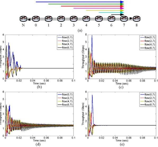
Fig. 2.5(a) shows a large parking lot scenario where there are containing 8 (0 ∼ 7), such as in Fig. 2.4 (a) but with various finite traffic demands, greedy stations, and Figs. 2.5 (b), 2.5 (c), 2.5 (d), and 2.5 (e) present throughputs of flow(0, 7), flow(2, 7), flow(4, 7), and flow(6, 7) at station 7 by AM, DBA, DMA, and FLAG, respectively. Assume that flow(0, 7) and flow(1, 7) require 2.1 Gpbs, flow(4, 7) and flow(5, 7) require 1.5 Gpbs, and flow(2, 7), flow(3, 7) and flow(6, 7) require 1.0 Gbps. It would be facts that station 6 will be the first one to incur congestion, and the added FE traffic flow to network at each station cannot always match its received fairRate due to the finite traffic demand at each station. Also, flow(0,7) and flow(1,7) will have the highest throughput when station 6 is in freecongestion or the remaining bandwidth is large because of their largest required traffic demands. It can be seen that at the first beginning, all flows just oscillate slightly, and then AM, DBA, and DMA oscillate all the ways, while FLAG can make all flows converge but takes 30 ms. It is because that FLAG indeed diminishes the effect of the propagation delay and generates the correct local fairRate at each agingInterval. Also, since each traffic flow is with different

finite traffic demand and is much less than that of the greedy case in Fig. 2.4(e), the damping amplitude is smaller than that in Fig. 2.4(e). Moreover, the FLAG stably realizes the RIAS fairness and has higher throughput by about 2.8%, 3.5%, and 2.4% than AM, DBA and DMA, respectively. On the other hand, the advertised fairRate by AM is often set as FullRate in this scenario because the bandwidth of the total demand traffic is 10.2 Gbps, slightly higher than the link capacity but much less than that of the greedy case in Fig. 2.4(b). In this situation, the aggregated traffic per agingInterval would be smaller, and the congestion, if any, could be solved by AM most of time. Thus, the flows by AM oscillate always and the flow(0,7) seriously oscillates due to its largest traffic demand. By DBA, its generation accuracy of local fairRate is susceptible to the propagation delay, as seen in Fig. 2.4. Also, in this scenario, station 0 and station 1 are the farthest ones to station 6 and flow(0,7) and flow(1,7) are with the largest traffic demand. These facts result in that flow(0,7) and flow(1,7) cannot be regulated by the station 6 quickly. This violent varying aggregation traffic per agingInterval and the effect of the propagation delay thus result in DBA generating the local fairRate improperly. Notice that if flow(0,7)requires less traffic demand, the oscillation amplitude of flows will be smaller. The DMA has the same phenomenon but its performance is better than DBA by 1.5% due to using the moving average technique.

Figure 2.5: (a) Large parking lot scenario with greedy traffic, and the throughput of (b) AM, (c) DBA, (d) DMA, and (e) FLAG in a large parking lot scenario with

various finite traffic flows.

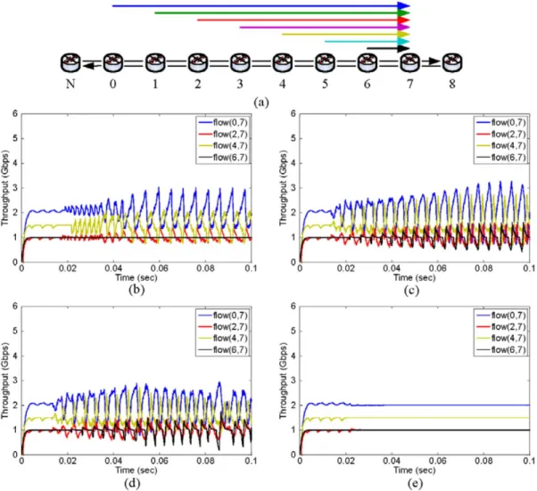
Fig. 2.6(a) shows an available bandwidth reclaiming scenario where there are 9 stations with finite traffic demand and a spatial reuse of flow(a,2) occurs, and Figs. 2.6 (b), 2.6 (c), 2.6 (d) and 2.6 (e) present the throughput of flow(a,2) at station and flow(0,7), flow(1,7), flow(2,7), and flow(6,7) at station 7 by AM, DBA, DMA, and FLAG, respectively. In this scenario, the flow(a, 2) requires 5.9 Gpbs, and similar to Fig. 3.11, flow(0, 7) and flow(1, 7) require 2.1 Gpbs, flow(4, 7) and flow(5, 7) require 1.5 Gpbs, and flow(2, 7), flow(3, 7), and flow(6, 7) require 1.0 Gbps. It can be seen that, just as in Fig. 3.11, at the beginning, all flows of all algorithms oscillate slightly, and finally FLAG makes all flows stabilize but takes 78 ms, while AM, DBA, and DMA oscillate all the ways. The reasons that all algorithms in this scenario behave worse than in the large parking lot scenario withvarious finite traffic flows, given in Fig. 2.4, are as follows. Since flow(a,2) is sunk at station 2, station 1 would have more

transient FE traffic flows than station 2, where station 1 has 10.1 Gbps traffic flow maximum, while station 2 has 5.2 Gbps traffic flow maximum. This phenomenon is conversed in Fig. 2.5, where station 1 has 4.2 Gbps traffic flow maximum, while station 2 has 5.2 Gbps maximum. Therefore, the station 1 in Fig. 3.13 will more frequently and heavily regulate its station 0, which has 5.9 Gbps transient traffic flow and 2.1 Gbps local traffic flow, than the station 1 in Fig. 5 will regulate its station 0, which has only 2.1 Gbps local traffic flow. Thus it can be believed that all flows in Fig. 2.6 would oscillate worse than in Fig. 2.5 for all schemes. Moreover, according to our computation, the throughput at station 6 by FLAG is about 0.990, which is higher than AM’s 0.825, DBA’s 0.914, and DMA’s 0.933. The reasons would be the same as those given before and are not mentioned again here.

Figure 2.6: (a) Available bandwidth reclaiming scenario with finite traffic demand, and the throughput of (b) AM, (c) DBA, (d) DMA, and (e) FLAG.

III. Intelligent Inter-Ring Route Control in Bridged Resilient Packet Rings

 System Model

A. Architecture of Bridge Node

Fig. 3.1 shows a bridge node connecting R0 and R1 RPR rings, where each ring contains a clockwise (CW) ringlet and a counter-clockwise (CCW) ringlet and there are M nodes on the ring. Assume that the fiber link capacity of the ringlet is C Gbps and the distance between every two consecutive nodes in the ringlet is the same. The proposed intelligent inter-ring route controller (IIRC) is installed in a spatially aware sublayer (SAS). As a new call request coming from one ring to the other, the IIRC will determine an appropriate ringlet for the inter-ring new call request. Also, the SAS forwards packets of existing calls to their interface in the bridge node based on the determined route. The bridge node has one interface associated each ringlet, and as shown in Fig. 3.2, each interface has two transit buffers: the ringlet and ingress buffers. The packets to the same ring are stored in the ringlet buffer, and those to the other ring are buffered in the ingress buffer.

Figure 3.1: Architecture of the bridge node

Each buffer contains a primary transit queue (PTQ) and a secondary transit queue (STQ). The high- (low-) priority packets, such as Class A and Class B-CIR (Class B-EIR and Class C), are stored in the PTQ (STQ). Voice packets, video packets of I-frame, video packets of B- or P-frames, and data packets are classified as Class A, Class B-CIR, Class B-EIR, and Class C, respectively. The bridge node always reserves bandwidth for the high-priority traffic. The scheduler in the bridge first serves the PTQs exhaustively with the round robin policy, and then serves the two STQs with the proportional round robin policy associated with their queue lengths.

Figure 3.2: Architecture of the interface

B. Fairness Algorithm

There are two fairness algorithms, called aggressive mode (AM) and conservative mode (CM), proposed in IEEE 802.17 standard [17], and another fairness algorithm, called distributed bandwidth allocation (DBA), proposed by Alharbi and Ansari. For simplicity, we adopt the AM fairness algorithm in each node for simulations. The AM fairness algorithm is described as follows. As specified in, if a node finds that its STQ queue length is longer than a threshold, it regards that congestion occurs and will initiate the AM fairness algorithm to limit its upper node’s add rate of the low-priority traffic to relieve congestion. The AM generates a limited value, called fairRate whose value is the available add rate of the low-priority traffic of node, each frame time period 100 μs. If a node finds that its upper node’s forward rate is less than its received fairRate, it will release the upper node’s add rate limitation by sending a fairRate with a special value, called FullRate, and the service rate of the node is the total link capacity C. If the received fairRate is not a FullRate, the node will limit its adding rate, which is bounded by the received fairRate, into the ring, and the service rate of the node is the summation of the arrival rate to the STQ, its received rate, and the reserved rate for high-priority traffic.

C. Intelligent Inter-Ring Route Controller

The intelligent inter-ring route controller (IIRC) is to determine a proper ringlet (CW or CCW) for an incoming inter-ring new call request at bridge. The determination of ringlet is based on the load balancing principle, in which the CW or CCW ringlet with lower congestion degree and higher service rate will be chosen. The congestion may come from the bridge node or the CW (CCW) downstream node. The former is related with the two STQ lengths of the associated interface in the bridge

node given in Figs. 3.1 and 3.2. Thus as shown in Fig. 3.3, the IIRC designs a fuzzy

bridge-node congestion indicator (FBCI) to intelligently detect this congestion. The

latter is related with the received fairRate from the downstream node of the associated ringlet. Therefore, the IIRC designs a PRNN (pipeline recurrent neural networks)

downstream-node fairness predictor (PDFP) to predict the CW or CCW

downstream-node congestion degree. Finally, the IIRC designs a fuzzy route

controller (FRC) to determine a proper ringlet for the incoming inter-ring new call

request. It receives the congestion indication from FBCI, denoted by CI , and the predicted mean received fairRate from PDFP, denoted byR_f , as input linguistic variables. Also, it considers the service rate of the CW or CCW ringlet at the bridge node, denoted by R, and the number of hops between the bridge and the destination, denoted by H, as input linguistic variables. Notice that the ringlet service rate at the bridge node is related with the received fairRate and more hops consume more system bandwidth. The FRC calculates the preference value of route, denoted by Pv, for CW and CCW interfaces and selects the ringlet with larger Pv as the proper ringlet route for the incoming inter-ring new call request.

Figure 3.3: Intelligent inter-ring route controller (IIRC)  Fuzzy Bridge-Node Congestion Indicator (FBCI)

The fuzzy bridge-node congestion indicator (FBCI) considers four measures as the input linguistic variables to determine the congestion degree of the bridge node at the CW or CCW interface. They are STQ lengths in the ingress buffer and the ringlet buffer, denoted by QSI and QSR, respectively, the amount of the reserved bandwidth for

high class traffic (which are stored in PTQ), denoted by BA, and the equivalent capacity of the incoming inter-ring new call, denoted by Ec. Note that the equivalent capacity for a new call can be estimated from its traffic description parameters: the peak rate, mean rate, and peak rate duration of packets. Among the four measures, the two STQ lengths are the more essential measures to indicate the degree of the congestion in the RPR bridge node. The BA occupancy is highly correlated with the STQ due to the fact that the system bandwidth is allocated to high priority traffic first. Also, the amount of Ec can cause the increment of the STQ length. The output linguistic variable of the FBCI is the congestion degree of the CW or CCW interface of the bridge, denoted by CI.

Term sets for the four input linguistic variables and the output linguistic variable are defined as T(QSI(QSR)) = {Short (S), Medium (M), Long (L)}; T(BA) = {Few (Fw), Many (Ma)}; T(Ec) = {Small (S), Large (L)}, and T(CI) = {Very Low (V L), Low (L), Medium (M), High (H), Very High (VH)}.

Here, the triangular function f









g are used to define the membership functions for the terms in the term set. These two functions are

0 0 0 0 0 0 0 0 1 0 0 1 1 1, for , ( ; , , ) 1, for , 0, otherwise. x x x a x x a x x f x x a a x x x a a   _{   }     _         _(3.1) and 0 0 0 0 0 0 1 0 1 0 1 1 1 1 1 1 1, for , 1, for , ( ; , , , ) 1, for , 0, otherwise x x x a x x a x x x g x x x a a x x x x x a a   _{   }        _  _{   }    _(3.2)

where x0 in f

 

 

)

0.25

0,

,

0.25

0,

;

(

)

(

l

l

L

Q

g

Q





 ,where Ls is the STQ queue size, and lth is the threshold in percentage. Note that if the STQ length is larger than lth · Ls, the bridge is in congestion and the fairness algorithm will be enabled. Membership functions for S, M and L in T(QSR) are similar to S, M and L in T(QSI), respectively. Membership functions for Fw and Ma in T(BA) are defined as _Fw(B_A)g(B_A ;0,0.025C ,0,0.025C) and _Ma(B_A)g(B_A ;0.1C,C ,0.075C,0) , where C is the link capacity. Membership functions of terms in T(Ec), are defined as

) R 0, , R 0, ; ( ) (Ec g Ec _{voice video} S 

 and )_L(Ec) g(Ec ;R_h ,C,R_video ,0 , where Rvoice and Rvideo are the minimum demand of the mean rates of the voice and video traffics, respectively, and Rh is the maximum demand of the mean rate of the video traffic to provide the high quality video. Membership functions for terms of output linguistic variable CI are defined as VL(CI) f(CI ;0.1,0,0) , L(CI) f(CI ;0.3,0,0) ,

) 0 0, 0.5, ; ( ) ( _{I I} M C  f C  , _H(C_I) f(C_I ;0.75,0,0), )_VH(C_I) f(C_I ;1,0,0 .

Table 3.1: The Fuzzy Rule base of FBCI

As shown in Table 3.1, there are 24 fuzzy rules for FBCI, where the notation ”X” in this table represents ”don’t care” of the linguistic variable. The order of significance of the input linguistic variables for the FBCI would be QSI, QSR, BA, and

Ec in sequence. The bridge will be in high degree of congestion if its two STQ queue

lengths are close to or longer than the threshold (the corresponding terms of QSI and

QSR, are Medium or Long). Finally, FBCI adopts the max-min method for fuzzy inference. The defuzzification method adopted is the center of area defuzzification

method.

 PRNN Downstream-Node Fairness Predictor (PDFP)

The bridge uses the received fairRate from associated ringlet of downstream node to discern the congestion degree of the downstream node. If the received fairRate is high, it means that the downstream nodes’s STQ can accept more flows and the bridge can raise its service rate. Otherwise, it means that the downstream nodes’s STQ is going to be full or has overflowed and the bridge should decrease its service rate. However, by the AM fairness algorithm considered here, thereceived fairRate would vary. This high variation of the received fairRate would make the bridge not easily detect if its downstream node is in congestion or not. Therefore, we originally choose an average received fairRate over the past m periods from the current nth period, denoted by R_f(n), as the input variable, where m is the size of the observation window, m ≥ 1. The R_f(n) could be appropriate to detect the congestion situation of the downstream nodes during a period and it is expressed by

m m n R n R n R n R f f f f ) 1 ( ) 1 ( ) ( ) (        ,

where Rf (n) is the received fairRate at time n. Also, since the bridge node routes the traffic flows call by call, the next-step mean received fairRate could be more appropriate to determine the route for an accepted new call. Here, a pipeline recurrent neural networks (PRNN) is adopted to design the PRNN downstream-node fairness predictor (PDFP). The fairRate with one-step prediction as a function of p received fairRates and q previously predicted fairRate, denoted by R_f(n1) or R_f for convenience, is given by )) 1 ( , . . . ), ( ); 1 ( , . . . ), ( ( ) 1 (          q n R n R p n R n R H n R_{f f f f f}

where R_f(i) is the previously predicted mean fairRate at ith period, n−q+1 ≤ i ≤ n, and H(·) is an unknown nonlinear function to be determined. The pipeline recurrent neural network (PRNN) prediction is a fast, low-complexity, and non-linear one that can approximate the function H(·).

The incremental change of synaptic weights is according to the steepest decent method. Also, the training of PRNN consists of two stages. During the off-line training phase, the PRNN, fed with the received fairRates, adjusts the synaptic weights recursively until the root mean square error (RMSE) of the desired prediction output is lower than the criteria. During the on-line training phase, the PRNN fairness

predictor obtains the fairRate predictions at (n+1)th period, R_f(n1), from the output of the first neuron of the first module, and receives the new fairRate R_f(n1); then it adjusts the synaptic weights using the real time recurrent learning (RTRL) algorithm. Due to the on-line learning capability, PDFP can adapt its wights to the current load conditions other than those set in the off-line training phase. If a PRNN contains q modules and M neurons per module, the computational complexity would be O(qM4). However, when the system is in operation and the PRNN has determined each parameter by learning, the computational complexity is reduced to O(1).

 Fuzzy Route Controller (FRC)

The fuzzy route controller (FRC) is to determine the route preference values, Pvs, for both of CW and CCW ringlets. The determination is based on four input linguistic variables of ringlet: the congestion indication of the bridge node, CI , the predicted mean received fairRate, R_f , the current service rate of the ringlet, R, and the number of hops to destination, H. The higher value Pv of a ringlet means that the ringlet is more suitable to accept the incoming new call request. Term sets for the input and output linguistic variables are defined as T(CI) = {Low (Lo), Medium (Me), High (Hi)}, T(R_f ) = {Small (Sm), Medium (Me), Large (La)}, T(R) = {Low (Lo), High (Hi)}, T(H) = {Few (Fw), Many (Ma)}, and T(Pv) = {Unsuitable (U), Weakly Unsuitable (WU), Weakly Suitable (WS), Suitable (S)}. Membership functions for terms of Lo,Me, and Hi in T(CI) are defined as _Lo(C_I)g(C_I ;0,0.25 ,0,0.25),

) 0.25 , 0.25 0.5, ; ( ) ( _{I I} Me C  f C  , and _Hi(C_I)g(C_I ;0.75,1 ,0.25,0). Membership functions for terms of Sm, Me, and La in T( R_f ) are expressed as

) 0.25 0, , 0.2 0, ; ( ) (R_f g R_f v v Sm     , _Me(R_f) f(R_f ;0.5v ,0.25v ,0.25v) , and ) 0 , 0.1 , , 0.6 ; ( ) (R_f g R_f v v v La   

 , where v denotes the unreserved bandwidth for the low priority traffic at the bridge node and v = C − BA.

Similarly, membership functions for T(R) are defined as ) 0.25C 0, 0.25C, 0, ; ( ) (R g R Lo   and _Hi(R)g(R ;0.6C,C,0.2C,0), where C is the total capacity of the fiber link. Membership functions for terms of Fw and Ma in T(H) are defined as _Fw(H)g(H ;0,N/3,0,N/3) and

0) /3, , /3, 2 ; ( ) (H g H N N N Ma 

 , where N is the total number of nodes in a RPR network. Finally, membership functions for terms in T(Pv) are defined as