Two essays of the market friction effects on asset prices: evidence from syndicated loan and futures markets

全文

(1)國立政治大學財務管理研究所博士論文. Two Essays of the Market Friction Effects on Asset Prices: Evidence from Syndicated 治 and Futures Markets 政 Loan. 大. 立. ‧. ‧ 國. 學. n. er. io. sit. y. Nat. al. Ch. engchi. 指導教授：張元晨研究生：吳偉劭. i n U. 博士撰. 中華民國一百零一年七月. v.

(2) 立. 政治大. ‧. ‧ 國. 學. n. er. io. sit. y. Nat. al. Ch. engchi. i n U. v.

(3) 謝辭一個人一個故事，每個生命的背後都有她自己獨特的故事，我也努力的寫著屬於自己的故事，不求故事有多精彩，只求可以感動自己，感動那些我看重的人，於是我不停筆的寫著，我知道，在寫這則故事的過程中我得到很多，也失去了不少，我都知道！故事寫到這，我暫時停筆，因為我想停下腳步來感謝一些人！猶記得十年前自己最常思考的問題就是“我到底想要做什麼？＂這個問題在十年前困擾自己很深，就在靈光一現的過程中，我循著上天的指引，辭去銀行的工作，一步無悔的走進研究所，從碩士班開始，轉眼間博士學位也要完成了；. 政治大現實環境總是嚴苛無情的考驗著每個人的意志力，如果不小心忘了初衷，很容易立. 對自己而言，取得博士學位是一種事業的選擇，而不是為了享有博士的虛榮，但. ‧ 國. 學. 就會迷失、迷惘，所幸世間有惡必有善，上天在不斷考驗你的同時，也派了許多天使來引導你，對於這些天使，我要表達自己最深切的感恩！. ‧. 首先，我要感謝在上天一直看顧我的父母，我把對你們的思念全部化為勇往. sit. y. Nat. 直前的力量，再艱難的挫折，我都因你們而勇敢！我要感謝我大哥、大姊、二姊、. al. er. io. 三姊，你們是我最強有力的後盾，謝謝你們對我任何的決定都是那麼的支持，沒. v. n. 有你們的支持我走不到今天，我任何的榮耀，都是屬於你們的。. Ch. engchi. i n U. 我要感謝我的指導老師張元晨老師、劉玉珍老師、李怡宗老師，你們不但在做學問上讓我得到最多的學習，在生活上也給我極大的支持，我在你們身上學到的，早已超越學術的範疇，你們是我將來有機會為人師表最佳的典範，將來我必以相同的胸襟對待自己的學生；我要感謝杜化宇老師，謝謝杜老師對我的信任與提攜，這份恩情我會永遠銘記在心；我還要回過頭感謝我的碩士班指導老師陳樹衡老師，謝謝陳老師在我碩士階段的照顧，在陳老師身上學到的精神永植我心！我要感謝文謙學長，除了平常學問的切磋之外，也在我挫折最多的時候給我最大的安慰，沒有你，我不曉得該如何排解那一段苦悶；我要感謝我的博士班同學肇榮，猶記得那一年我們一起準備學科考，何媽媽的便當讓我免於除夕夜挨餓.

(4) 的窘境；感謝曉梅，我們總是可以掏心掏肺的聊天；感謝健偉，你總能用你開朗的天性驅散別人的憂鬱；感謝胤哲總是友善的面對每個人、感謝崇齡，女中豪傑的最佳典範，不論大家最後選擇了什麼路，那段有你們的時光，是再怎麼艱辛彼此都不孤單的時光；我要感謝系辦的助教郁芳及雪玲，謝謝你們凡事都那麼的幫忙；我要感謝淑華、楚彬、還有玉美學姊，你們給我極多的幫助，雖然我很少表達什麼，但很多事我都感受在心裡；我要感謝所有財管系博士班的成員美菁、苡文、周燕、富德…，謝謝你們這些日子所帶來的歡笑、汗水、甚至淚水，也謝謝你們對我的諸多包容。. 治政大俊緯，謝謝你們義氣相挺，從碩士班一路陪我到博士班；也謝謝以前經研所的學立我還要感謝我的幾位碩士班同學，惟毅、毓芝、仁傑、家綺、秋媚、顯一、. 長科宏、秉聰；我要感謝吳經理，謝謝你多年來的關照，跟你在形而上想法的交. ‧ 國. 學. 流，讓我對生命有更深切的體悟，你是我另類的指導老師；我還要感謝更多更多. ‧. 的人…. y. Nat. 要感謝的人太多了，這一刻才發現自己是何等渺小，為了完成屬自己個人的. al. er. io. 於這個社會！. sit. 階段性任務，竟然需要集結那麼多人的力量，希望自己將來有能力可以加倍回饋. n. v i n 故事寫到這裡，我合上書本，不是結束，而是即將開啟新頁；謝謝在這塊土 Ch engchi U. 地上曾經陪伴過我的一切，另一塊土地正在等著我，無論走到哪我都會繼續寫著屬於自己的故事，也希望有機會可以常常回過頭來聽聽大家的故事！.

(5) Preface In this dissertation, two essays are used to illustrate how market friction would influence asset prices. In the first essay, I use the data from the U.S. syndicated loan market to show how communication barriers among lenders would affect their decisions, which in turn affect loan spreads. If potential lenders can’t freely communicate with each other, those who make decision after will learn by observing the decisions of their predecessors. Once their own signals are dominated by the information revealed by their predecessors’, those who act later will rationally ignore. 政治大 In the first essay, I will show how cascade effect can influence loan spreads and 立. their own signals and follow suit. In economics, this is called “informational cascade.”. non-price contract terms.. ‧ 國. 學. In the second essay, I use the data from Taiwan Futures Exchange to examine. ‧. the lead-lag relationships between the index futures returns, index futures volume, and. y. Nat. spot returns. The lead-lag relationship depends on which venue informed traders will. er. io. sit. choose to trade and informed traders’ choice may depend on short sale constraints, transaction costs, leverage effect, and so on. In my second essay, I will show which. al. n. v i n C htraders choose to U market is the venue the informed trade and which type of traders engchi tend to be informed traders.. The two essays of this dissertation have been transformed into working papers for conference presentation and journal submission. The first working paper based on Chapter II, The Cascade Effect in the Syndicated Loan Market, has accepted by the 19th Conference on the Theories and Practices of Securities and Financial Markets and is presented on 10th December 2011 in Kaohsiung. The second working paper based on Chapter III, The Relationships between the Futures Returns, Futures Volume, and Spot Returns, has been submitted to Journal of Financial Studies..

(6) 立. 政治大. ‧. ‧ 國. 學. n. er. io. sit. y. Nat. al. Ch. engchi. i n U. v.

(7) Abstract Two essays are comprised in this dissertation to explore how market friction affects the processes of price formation. The first essay investigates on both theoretical and empirical bases how segmentation of communication amongst potential lenders can influence loan contracts. Two cases are considered. The first one assumes that potential lenders can freely communicate with each other; the second one assumes that each potential lender can only observe the decisions of its predecessors. I show theoretically that the ex post observed interest rate will be higher. 政治大 communicate freely with each other. These predictions are confirmed by my empirical 立. and the probability of syndication failure will be lower if the potential lenders cannot. work. Using a novel proxy, relational distance, for the segmentation of. ‧ 國. 學. communication, I show that the larger the relational distance, the higher is the loan. ‧. spread and the lower is the probability of syndication failure. In addition, the. y. Nat. relational distance is positively correlated with the probability of the existence of. er. io. sit. non-price contract terms, such as the requirement for collateral and guarantees. My conclusions are found to be robust to endogeneity issues, potentially omitted variables. n. al. Ch. and alternative model specifications.. engchi. i n U. v. The second essay focuses on the informational effects between futures market and its spot market. Intraday data are used to investigate the lead-lag relationship between the TX returns, the TX trading activity and the TAIEX stock index returns. I focus on the transmission direction and the source of information and find that there are specific lead-lag relationships between futures returns and spot returns, in addition to the contemporaneous relationship predicted by carry-cost theory and efficient market theory. The results show that futures returns significantly lead spot returns, which suggests that informed trades occur in the futures market and makes information flows from the futures market to the spot market. By distinguishing.

(8) different types of futures traders and using private information, net open buy, as a proxy for futures trading activity, I found that the major source of informed trades is foreign institutional traders because their trading activity have predictive power for future movements in both spot and futures prices. In contrary, traders in the other categories carry no information about the directional changes in both spot and futures prices.. 立. 政治大. ‧. ‧ 國. 學. n. er. io. sit. y. Nat. al. Ch. engchi. i n U. v.

(9) Table of Contents Chapter I. Introduction ................................................................................................... 1 Chapter II. The Cascade Effect in the Syndicated Loan Market ................................... 5 1. Introduction ............................................................................................................ 5 2. The Model............................................................................................................. 10 2.1. Perfect Communication .................................................................................. 11 2.2. Informational Cascades .................................................................................. 12 3. Empirical Framework ........................................................................................... 14. 政治大. 3.1. Proxies for the degree of segmented communication .................................... 14. 立. 3.2. Loan syndication networks ............................................................................ 15. ‧ 國. 學. 3.3. Hypotheses ..................................................................................................... 18 3.4. Empirical specifications ................................................................................. 19. ‧. 4. Data and Descriptive Statistics ............................................................................. 21. y. Nat. sit. 5. Empirical Results .................................................................................................. 23. n. al. er. io. 5.1. Results for Physical Distance ......................................................................... 23. i n U. v. 5.2. Results for Relational Distance ...................................................................... 26. Ch. engchi. 5.2.1. Relational distance and loan spreads ....................................................... 26 5.2.2. Relational distance and non-price requirements ...................................... 28 5.2.3. Relational distance and syndication failures ............................................ 30 5.3. Robustness checks .......................................................................................... 31 5.3.1. Alternative explanations and model specifications.................................. 31 5.3.2. Endogeneity ............................................................................................. 34 5.3.3. Omitted variables ..................................................................................... 36 6. Conclusions .......................................................................................................... 37 Appendix A............................................................................................................... 51 i.

(10) Appendix B ............................................................................................................... 53 Chapter III. The Relationships between Futures Returns, Futures Volume, and Spot Returns: Evidence from Taiwan Futures Market ..................................... 65 1. Introduction .......................................................................................................... 65 2. Empirical Specifications ....................................................................................... 69 3. Data and Preliminary Analysis ............................................................................. 72 4. Empirical Results .................................................................................................. 76 4.1. The lead-lag relationship between index returns, futures returns, and overall. 政治大 4.2. The differences in information content of the four trader classes .................. 78 立. net open buy................................................................................................... 76. 4.2.1 The spot market......................................................................................... 79. ‧ 國. 學. 4.2.2 The futures market .................................................................................... 81. ‧. 4.2.3 Robustness check ...................................................................................... 82. y. Nat. 4.3 VAR Results.................................................................................................... 83. er. io. sit. 5. Conclusions .......................................................................................................... 88 Appendix A............................................................................................................... 97. al. n. v i n Ch Chapter IV. Conclusions ............................................................................................ 107 engchi U. Reference……………………………………………………………………………111. ii.

(11) List of Tables Table 2.1: Descriptive statistics of regression variables .............................................. 42 Table 2.2: Effects of physical distance on loan contract terms and syndication failures ....................................................................................................................... 43 Table 2.3: Effect of relational distance on loan spreads .............................................. 44 Table 2.4: Effects of relational distance on non-price contract terms ......................... 45 Table 2.5: Effect of relational distance on syndication failures................................... 47 Table 2.6: Robustness check: alternative explanations and model specifications ....... 48. 政治大 Table 2.8: Robustness check: 立omitted variables .......................................................... 50 Table 2.7: Robustness check: endogeneity .................................................................. 49. ‧ 國. 學. Table B1: Variable definitions ..................................................................................... 53 Table B2: Effects of physical distance on loan contract terms and syndication failures:. ‧. Facilities without foreign lender .................................................................... 54. sit. y. Nat. Table B3: Effects of physical distance on loan contract terms and syndication failures:. al. er. io. Facilities with foreign lenders ....................................................................... 55. v. n. Table B4: Effects of physical distance on loan contract terms and syndication failures:. Ch. engchi. i n U. Big loans ........................................................................................................ 56 Table B5: Effects of physical distance on loan contract terms and syndication failures: Small loans .................................................................................................... 57 Table B6: Distribution of loan failures ........................................................................ 58 Table B7: t-test of paired sample of syndication failure and success. ......................... 58 Table B8: Complete results of Table 2.6, Panel A ...................................................... 59 Table B9: Complete results of Table 2.6, Panel B ....................................................... 60 Table B10: Complete results of Table 2.6, Panel C ..................................................... 61 Table B11: Complete results of Table 2.6, Panel D .................................................... 62 iii.

(12) Table B12: The first-stage results of instrumental regression ..................................... 63 Table B13: The second-stage results of instrument regression ................................... 64 Table 3.1: Summary statistics of the TX transactions ................................................. 91 Table 3.2: Autocorrelations of the spot returns and futures returns ............................ 92 Table 3.3: Regression results of the spot returns on the futures returns and net open buy ................................................................................................................. 93 Table 3.4: Regression results of the spot returns on the net open buy of the four trader classes ............................................................................................................ 94. 政治大 classes ............................................................................................................ 95 立. Table 3.5: Regression results of the TX returns on the net open buy of the four trader. Table 3.6: Vector autoregression (VAR) results.......................................................... 96. ‧ 國. 學. Table A1: Unit root tests .............................................................................................. 97. ‧. Table A2: VAR results – unclassified data .................................................................. 98. y. Nat. Table A3: Robustness check of Table 3.4 ................................................................... 99. er. io. sit. Table A4: Robustness check of Table 3.5 ................................................................. 100 Table A5: VAR results – excluding the futures returns ............................................. 101. al. n. v i n C hthe spot returns ................................................. Table A6: VAR results – excluding 102 engchi U. Table A7: Granger test I ............................................................................................ 103 Table A8: Granger test II ........................................................................................... 104 Table A9: Granger test III .......................................................................................... 105 . iv.

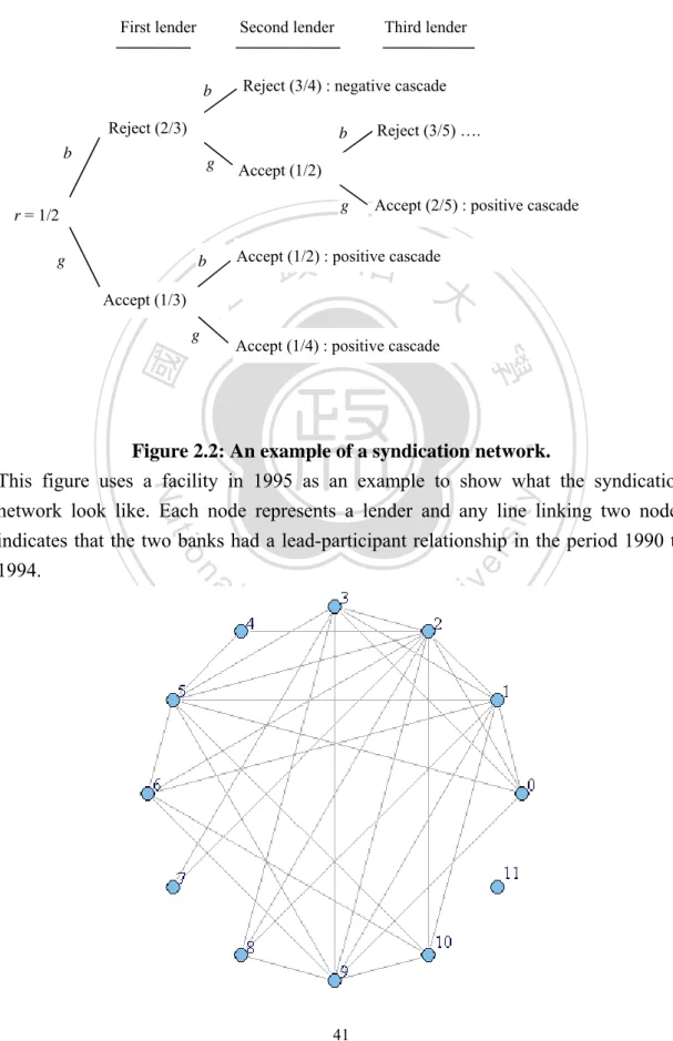
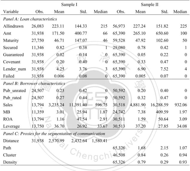
(13) List of Figures Figure 2.1: An example of the decision rule of the cascade case ................................ 41 Figure 2.2: An example of a syndication network. ...................................................... 41. 立. 政治大. ‧. ‧ 國. 學. n. er. io. sit. y. Nat. al. Ch. engchi. v. i n U. v.

(14) 立. 政治大. ‧. ‧ 國. 學. n. er. io. sit. y. Nat. al. Ch. engchi. vi. i n U. v.

(15) Chapter I Introduction In a frictionless market, price should perfectly aggregate information held by market participants and reflect an asset’s true value. Moreover, in two related markets such as a spot market and its derivative market should impound information simultaneously so that there is no lead-lag relationship between their price adjustments. However, market friction such as transaction costs, communication. 政治大 of price formation and price 立discovery. This dissertation uses two markets, the U.S.. barriers, trading limitations, illiquidity, and market structure often affects the process. ‧ 國. 學. syndicated loan market and Taiwan Futures market, to illustrate the effects of market friction on asset prices. There are two essays in this dissertation. In the first essay, I. ‧. extend Welch (1992)’s model to the syndicated loan market to show how. sit. y. Nat. segmentation of communication can affect lending conditions, especially loan spreads.. al. er. io. Two cases are considered. The first case assumes all potential lenders can freely share. v. n. their information with each other. In the second one, I assume each potential lender. Ch. engchi. i n U. can only observe the decisions of her predecessors. By extending Welch’s model, I show that if potential lenders can freely share their information about the borrower, the ex-post observed loan spreads are lower and probability of syndication failures is higher. The intuition is that in the second case the lead bank will increase the interest rate to elicit a positive cascade and make failure become impossible. Using relational distance as a proxy for segmentation of communication, the model’s predictions are confirmed by my empirical work. The first essay contributes to the extant literature in three ways. First, to my best knowledge, this is the first study to explore cascade effect in the syndicated loan 1.

(16) market. Although some studies have examined the herd behavior in banks’ investment decisions (e.g., Jain and Gupta, 1987; Nakagawa and Uchida, 2003; Uchida and Nakagawa, 2007; Acharya and Yorulmazer, 2008), they did not explore how herd behavior affects loan pricing. Second, several distance measures have been proposed and associated with economic decisions, for example, physical distance (Mian, 2006; and Giannetti and Yafeh, 2012), distance of specialization (Cai et al., 2011), and cultural distance (Giannetti and Yafeh, 2012). Also, many studies suggest that a tight relationship. 政治大 (e.g., Baum et al., 2004; Hochberge et al., 2007; Cohen et al., 2008; and Meuleman et 立. between economic agents favors communication and the dissemination of information. al., 2009). We extend these ideas to propose a novel proxy, relational distance. It is. ‧ 國. 學. difficult to capture relationships amongst economic agents and to quantify the. y. Nat. analysis.. ‧. relational distance. We overcome these obstacles by conducting a social network. er. io. sit. Third, to my best knowledge, this essay is also the first study to empirically test the determinants of syndication failures. It is an important issue because syndication. al. n. v i n Cand failures are costly to borrowers and may impair investment activities. U h elenders i h ngc Understanding the causes of syndication failures helps to improve the success of the syndicated loan market. In the second essay, I study the lead-lag relationship between Taiwan futures market and its spot market. According to the carry-cost theory, if the markets are frictionless, contemporaneous returns in the futures market and spot market would be perfectly correlated (Stoll and Whaley, 1990). However, transaction costs (such as fees and taxes), trading limitations (such as limitation on short sales), or the transaction characteristics of the asset itself (such as leverage effect) may cause one market to react faster to information than the other. In this essay, I show that the 2.

(17) futures returns strongly lead its spot returns and this phenomenon is driven by the trading activity of foreign institutional traders. By distinguishing the trading volumes of different trader types, I found the net open buy of foreign institutional traders in futures market have predictive power for not only the spot returns but also the futures returns. In contrary, traders in the other categories make no directional prediction on both spot and futures returns. The main contributions of the second essay come from three aspects. First, unlike the previous literature simply discusses the lead-lag relationship between. 政治大 futures trading volume, I simultaneously explores the information content regards to 立. futures price changes and spot price changes or between futures price changes and. the futures returns and spot returns, futures trading activitiy and spot returns, and. ‧ 國. 學. futures returns and futures trading activity. It is important to analyse the relationships. ‧. between the futures trading activity, futures returns, and spot returns at the same time.. y. Nat. Only considering the relation between the two market returns, we cannot determine. er. io. sit. who tend to be informed traders. Simply examining the relation between the futures trading activity and futures returns, it is hard to conclude that informed traders do. n. al. Ch. choose futures market to trade in first.. engchi. i n U. v. Second, past literatures specifically explored the relationship between the options trading activity and spot price changes. Under the situation where it is impossible to distinguish the types of trader, they mainly use the overall market trading activity as their analysis basis. Because it is impossible that every trade is informed trade, this choice will affects the credibility of the result, or even inconsistent explanations appear (e.g. EOS and CCF). In view of this, I not only study the relationship between the overall futures market trading activity and the spot price changes, but also further explores whether different identities of traders have different information content. 3.

(18) Third, in the research of trading activity, most literatures use the total trading volume directly (e.g. Though Sadath and Kamaiah, 2009; Anthony, 1988; Stephan and Whaley, 1990), or divide trading into buyer-initiated and seller- initiated (e.g. EOS; CCF). Pan and Poteshman (2006), however, found that observing the signal quality of these variables is inferior to dividing the opening and closing trades. Therefore, I uses non-public information, net open buy (open-buy volume minus open-sell volume), as the analysis variable of the futures trading activity, which can better capture the informed trades on the market.. 政治大 investigates how cascade effect can happen in syndicated loan market and how the 立. The remainder of this dissertation is structured as follows: Chapter II. effect can affect the loan contract terms and the probability of syndication failure.. ‧ 國. 學. Chapter III examines the lead-lag relationships between the price movements of. ‧. futures market and its spot market and the volumes of different classes of futures. n. al. er. io. sit. y. Nat. traders. Chapter IV summarizes the results and concludes this dissertation.. Ch. engchi. 4. i n U. v.

(19) Chapter II The Cascade Effect in the Syndicated Loan Market. 1. Introduction The imitation in economic decision-making is prevalent in human society. It is found in choice of restaurants, schools, political candidates, research topics, investments, and initial public offerings (Banerjee, 1992; Shiller, 1995). However, it. 治政 does not necessarily imply that imitators are irrational.大 When people make decisions 立 in sequence and are subject to imperfect signals, they often take account of the ‧ 國. 學. information revealed by the actions of others. If their own signals are dominated by. ‧. information stemming from the actions of their predecessors, those who act later may rationally ignore their own signals to follow suit. This phenomenon is the so-called. y. Nat. io. sit. informational cascade or herd behavior.. n. al. er. Welch (1992) developed a theoretical model to illustrate the role of information. Ch. i n U. v. in generating cascades. Using the example of the IPO market, Welch showed that. engchi. with perfect communication amongst all investors, all successful offerings by a risk-neutral uninformed issuer are underpriced. In the absence of perfect communication from early to late investors but allowing for late investors to observe the decisions of early investors, this can give rise to either positive or negative cascades. Given the high likelihood of a negative cascade originating, in which there is no buyer independent of the signal received, there is a tendency for sellers to under price so that all goods are sold. The model of Welch has been applied to the insurance market for special risks by D’Arcy and Oh (1997). In this paper, I extend Welch’s. 5.

(20) model to the U.S. syndicated loan market. My goal is to show that the cascade effect also affects loan pricing and the probability of syndication failure. A syndicated loan is a loan that is provided by a group of lenders and is structured by one or several commercial or investment banks known as lead banks. In the syndication process, once the mandate has been awarded, the lead bank and the borrower establish a relationship and become “partners” (Sufi, 2007; Focarelli et al., 2008). After negotiating lending conditions and contract terms with the borrower, the lead bank turns to approach potential lenders. If potential lenders accept (or reject) the. 政治大 Whether informational cascades happen or not in the syndication process 立. invitation nonsynchronously, then informational cascades become possible.. depends on the scenarios of interaction amongst potential lenders. This is the first. ‧ 國. 學. issue I want to investigate. By extending Welch’s model, I show that if potential. ‧. lenders can freely share their information about the borrower, the probability of. y. Nat. syndication failure is always positive. This is because the loan spread which the lead. er. io. sit. bank sets may not be the same as one which reflects information held by all potential lenders. The probability that the former rate is lower than the latter is always positive.. al. n. v i n C hcan only observe the However, if each potential lender decisions of potential lenders engchi U. which were previously approached by the lead bank, the syndication is unlikely to fail. The intuition is that in this case the rational lead bank will set a higher loan spread to elicit a positive cascade in seeking to avoid costly failure. Accordingly, it is also reasonable to expect that the loan spread in this scenario will be higher than that where information is freely shared amongst potential lenders. The second issue I want to explore is whether my model’s predictions are supported in practice. I use two proxies, physical distance and relational distance, to empirically capture the segmentation of communication amongst potential lenders. Physical distance measures the average distance between the cities in which the 6.

(21) principal executive offices of the syndicate members are located. Long physical distances may impair communication. However, when it is examined, I find no evidence to support my model’s predictions. Indeed, progress and innovations in technology, transportation, and communication may make physical distance an unbinding constraint. Giannetti and Yafeh (2012) tested the effect of physical distance between the lead bank and the borrower on loan cost and their results are also insignificant. Relational distance captures the close relationship amongst potential lenders. 政治大 average path length, clustering coefficient, and density, are used to measure relational 立 arising from their collaboration over the preceding five years. Three variables,. distance. All of them are used in social network analysis. As stressed by Hochberg et. ‧ 國. 學. al. (2007, 2010) and Cohen et al. (2008), networks facilitate the sharing of. ‧. information. A tight relationship favors communication and the dissemination of. y. Nat. information. My empirical results confirm this hypothesis and support the model’s. er. io. sit. predictions. I find that relational distance affects not only loan spreads but also non-price contract terms. The longer the relational distance, the higher is the loan. al. n. v i n spread and the probability of C collateral or guarantees h e n g c h i U being offered. In addition, relational distance also affects the probability of syndication failure. The longer the relational distance, the lower is the probability that a syndication fails.. My paper is related to several strands of literature. The first one is the literature on herd behavior in the investment decisions of banks. Jain and Gupta (1987) tested the lending behavior of U.S. banks of different sizes and found weak evidence of herding in international lending decisions. Nakagawa and Uchida (2003) and Uchida and Nakagawa (2007) both demonstrated the existence of herd behavior between different types of Japanese banks. The evidence is affirmative. Acharya and Yorulmazer (2008) developed a model to show that the likelihood of information 7.

(22) contagion can induce bank owners to herd with other banks in investment decisions. While these papers investigate the herd behavior of banks in the choice of regions, industries, or portfolio, I study the decisions of banks as to whether they will join a lending syndicate. My results provide evidence of how the probability of cascade occurrence affects loan conditions and syndication failures. This paper is also related to the literature on financial networks. There are widespread examples of financial networks such as the coinvestment networks of venture capital firms (Hochberg et al., 2007, 2010), the links between mutual fund. 政治大 networks of investment banks in security offerings (Baum et al., 2004). Here, I focus 立 managers and corporate board members (Cohen et al., 2008), and the co-underwriting. on syndication networks of the loan market. I am not the first to study the networks in. ‧ 國. 學. the syndicated loan market. Based on the lead-participant relationship between banks,. ‧. Godlewski et al. (2012) constructed the networks in the French syndicated loan. y. Nat. market. They used three network centrality measures, betweenness, closeness, and. er. io. sit. degree, to proxy lenders’ experience and reputation, and demonstrate that they play a significant role in reducing loan spread. Cai et al. (2010) explored how networks are. al. n. v i n C hchoose their syndicate formed, that is, how lead banks partners. They found lead engchi U. banks are more likely to choose banks that have similar lending expertise and give these banks more senior roles in the syndicate. My paper is different from previous literature in several ways. While Godlewski et al. (2012) are concerned with the experience and reputation of lenders and use centrality measures as proxies, I am interested in how cascade effect can happen and how it can affect loan prices. I use the average path length, clustering coefficient, and density as proxies for segmented communication amongst lenders. Unlike Cai et al. (2010) who examined how distance of lending expertise can affect the future collaboration of lenders and loan spreads, I 8.

(23) study how the past collaborative relationships can affect the efficiency of sharing information, which in turn affects loan spreads. My paper is mainly related to the growing literature on syndicated loans. Many studies emphasize the effect of information asymmetry on loan spreads (e.g., Focarelli et al., 2008; Ivashina, 2009; Nandy and Shao, 2010) and the structure of loan syndicates (e.g., Sufi, 2007; Lee and Mullineaux, 2004; Esty and Megginson, 2003; Bosch and Steffen, 2011). I contribute to this literature by providing additional evidence that the cascade effect also plays an important role in resolving contract. 政治大 Ivashina and Sun (2010), Nandy and Shao (2010), and Nini (2008) paid attention 立. terms.. to the significant increase in institutional investors’ demand for loans and examined. ‧ 國. 學. the relationship between loan spread and institutional investment. Their evidence. ‧. shows that because of information asymmetry institutional loans have higher loan. y. Nat. spreads than bank loans (Nandy and Shao, 2010; Nini, 2008). In addition, the strong. er. io. sit. demand in institutional investors puts downward pressure on loan spreads (Ivashina and Sun, 2010). In this paper, I also investigate loan pricing and lenders’ behavior in. al. n. v i n C hnot restrict itself toUinstitutional demand. subscriptions, but my research does engchi. Finally, my work is also related to the article of Giannetti and Yafeh (2012).. They studied the effect of cultural distance between the lead bank and borrower on lending contracts. The motivation is that cultural differences between contracting parties may impede communication and cause friction. Their results show that the lead bank is prone to offer better loan conditions to culturally similar borrowers. My paper complements Giannetti and Yafeh’s work in at least two respects. First, while Giannetti and Yafeh concentrate on how cultural distance between lead bank and borrower can affect economic interaction, I focus on how relational distance amongst lenders can segment communication. Second, relational distance can be viewed as a 9.

(24) contributing factor which can impair communication even when there is no cultural difference. The remainder of this paper is organized as follows. Section 2 extends Welch’s model to the syndicated loan market. Section 3 introduces the empirical methodology. Section 4 describes the data and summary statistics. The empirical results and robust checks are presented in Section 5. I conclude this paper in Section 6.. 2. The Model Suppose a firm intends to invest in a project and decides to raise capital from the. 政治大 approach n other banks (potential lenders) to inquire whether they are willing to 立 syndicated loan market. It has chosen a lead bank. Assume the lead bank will. ‧ 國. 學. participate in the deal. If the return of the project is r p (e.g., IRR) then the borrower will not accept the loan interest rate, r, which is higher than r p . On one hand, the. ‧. interest rate r is the borrower’s financing cost and on the other hand, it reflects the. sit. y. Nat. borrower’s credit quality. Although the borrower’s credit quality is unobservable,. io. er. each bank knows its range, which lies somewhere between r g and r b with a. al. uniform distribution, and r b  r g . The higher the borrower’s credit quality the lower. n. v i n C borrower never accepts the interest rate will be. Since the h e n g c h i U an interest rate larger than r p , I also assume r b  r p . Now suppose each potential lender can observe its own signal s  {g , b}. independent of other banks’ signal. Here, g and b denote a good and bad signal, respectively. Define . as a linear transformation of. [r g , r b ]. such that. r  (1   )r g   r b .  can be viewed as the probability that a lender receives a bad signal, b. Since r and  have an one-to-one mapping, the loan interest rate can be expressed not only in terms of r but also in terms of  . For example, in the case of r b  r p , I can express r p in terms of  , that is  p  1 . 10.

(25) 2.1. Perfect Communication Consider the first case in which all potential lenders can fully communicate with each other and share information amongst themselves. Let k be the number of b signals under n possible lenders. The lowest interest rate, where each lender would accept given k bad signals for n potential lenders, is equal to the posterior expected value of  . If  is uniformly distributed in [0,1], the posterior expected value of  given k bad signals will be: E ( | k , n) . k 1 n2. (1). 政治大 each potential lender is willing to accept given k bad signals amongst n potential 立. This is the Lemma 1 of Welch (1992). Equation (1) is the lowest interest rate which. ‧ 國. 學. lenders.. According to the Lemma 2 of Welch (1992), the ex ante probability of observing. y. 1 n 1. (2). sit. Nat. prob( k b signals | n possible lenders ) . ‧. k bad signals is:. n. al. prob(k or less b signals | n possible lenders ) . Ch. engchi. k 1 n 1. er. io. and the ex ante probability of observing k or less bad signals is:. i n U. v. (3). Using equations (1) to (3), I can transform the borrower’s optimization problem over price into optimizing over the number of bad signal, k, by minimizing expected cost:  k 1 k 1   k 1  p min     1   k  n 1   n  2   n 1 . (4). Here, I assume that the borrower is risk neutral. The first term of equation (4) is the borrower’s financing cost multiplied by the probability that the borrower receives the loan. The second term is the opportunity cost of giving up the project, multiplied by the probability that the syndication fails. According to the first order condition, the optimal k is: 11.

(26) n  k *    1  p  1 2 . (5). Due to  p  1 , it follows that k *  n / 2 . According to equation (1), the optimal interest rate is r *  1 / 2 . In order to safeguard its reputation and to establish a good relationship with the borrower, I assume that the lead bank will choose this interest rate. Indeed, as noted by Focarelli et al. (2008), once the lead bank has been mandated, it will partner with the borrower to obtain a satisfactory result from the placement. 2.2. Informational Cascades Now I consider the case where the lead bank approaches potential lenders. 治政 sequentially. Each potential lender who is approached大 has to make a decision about 立 participating in the loan syndication and its decision is irreversible. In addition, each ‧ 國. 學. lender is fully informed of its own signal and previous lenders’ decision but not their. ‧. signals. In this situation, the decision made by the subsequent lender is dependent upon the action of earlier lenders. Once two consecutive lenders make the same. y. Nat. io. sit. decision, so will all subsequent lenders. That is, a cascade happens whenever a lender. n. al. er. ignores its own signal and relies only on the decisions of the earlier lenders. To see. Ch. i n U. v. how this could happen, I illustrate with the following examples.. engchi. Figure 2.1 provides the decision rule of each consecutive lender. Assume the lead bank sets a loan price at r =1/2. If the first lender approached by the lead bank holds a good signal (g), according to equation (2), the lowest interest rate for which the lender will accept is 1/3, so this bank will choose to participate in the loan syndication. If the second lender has a bad signal (b) and the lowest interest rate the second lender is willing to accept is 1/2, the bank can choose to participate or not participate in the deal. Suppose the bank chooses to participate in the loan syndication. Given that the two consecutive lenders have joined in the loan syndication, the third lender and all subsequent lenders will accept the deal no matter what their signals are. 12.

(27) This gives rise to a positive cascade in lending. If the second lender’s signal is good (g), the lowest interest rate the bank is willing to accept is 1/4. In this case, the second lender will accept the lead bank’s invitation to join in the loan syndication and a positive cascade ensues. [Insert Figure 2.1] Now consider another scenario where the first lender observes a bad (b) signal. The lower bound of the interest rate for which the first lender could accept is 2/3 hence the deal will be rejected. If the second lender also has a bad (b) signal, the deal. 政治大 than 3/4. In this scenario, the 立second lender chooses to reject the deal. Given that two will be accepted by this lender if and only if the loan interest rate is equal to or higher. ‧ 國. 學. consecutive lenders have rejected the deal, all subsequent lenders will also reject the deal regardless of their signals. This outcome results in a negative cascade. If the. ‧. second lender observes a good (g) signal instead of a bad (b) one, she will price the. sit. y. Nat. lending rate at 1/2 and will be indifferent to participating or not being a participant of. al. er. io. the loan syndication. Suppose the second lender decides to accept the deal, now that. v. n. the first lender is not willing to finance the project and the second lender chooses to. Ch. engchi. i n U. finance it, the cascade effect will not take place. If the third lender’s signal is good (g), it will accept the deal and a positive cascade will occur. However, if the signal is bad (b) the third lender will not participate in the loan syndication and, again, the cascade effect will not occur. In sum, whether a cascade happens or not depends on the ordering of signals of the consecutive lenders which the lead bank approaches. However, for the case where interest rate is higher or equal to 2/3, a positive cascade will take place with certainty. Following Theorem 5 of Welch (1992), a risk-neutral lead bank will optimally choose. 13.

(28) the interest rate of 2/3 which is the lowest interest rate a positive cascade will undoubtedly occur and the probability that the loan syndication will fail is zero. It is easy to see that the interest rate under the case of perfect communication is lower than the one under the cascade case. This always holds if the borrower is risk-neutral or moderately risk-averse. The intuition is that loan failures are costly for both borrowers and lead banks. Under the cascade case, the lead bank can completely rule out the possibility of syndication failure by increasing interest rates. This is impossible under the case of perfect communication because the probability of the. 政治大 should note that even though interest rate is lower under the case of perfect 立. syndication failure is always positive under the distributional assumption. However, I. communication than cascade cases, the expected cost of the former is in fact higher. It. ‧ 國. 學. can be seen from equation (4) that the expected cost is (3n  2) / (4n  4) for the case. ‧. of perfect communication. This implies that for n larger than 1, the expected cost will. y. Nat. be equal to or larger than 2/3. The bigger n is, the larger is the expected cost. In. er. io. sit. summary, I conclude that the ex post financing cost is lower under perfect communication than under cascade, although the ex ante cost of financing is higher. n. al. Ch. due to some probability of failure.. engchi. i n U. v. 3. Empirical Framework 3.1. Proxies for the degree of segmented communication To empirically test the model’s prediction, proxies that measure segmented communication amongst lenders are required. Two proxies, namely physical and relational distance, are used. Welch (1992) proposed the use of “locality” as a segmentation measure of communication. Following this idea, my first proxy is the physical distance amongst lenders. For a given facility (or tranche), I calculate the physical distance between pairs of lenders based on the cities of their principal 14.

(29) executive offices. After calculating all possible pairs, I then average the distance across all pairs and obtain the mean distance for lenders of the facility. The intuition is that the farther the physical distance amongst lenders, the more difficult they communicate with each other. One problem with the use of this proxy is that it may not truly reflect the ease of communication amongst lenders. In this day and age, innovations in technology, transportation, and communication may attenuate the constraint of physical distance, thus communication between two lenders that are located far apart may not necessarily be hindered by their physical distance. To. 政治大 relational distance amongst lenders. 立. circumvent the limitation of this proxy, I proposed a second proxy, which captures the. I assume that lenders who have collaborated in past syndications would be prone. ‧ 國. 學. to communicating and sharing their information with each other. To measure the. ‧. extent of collaborative relationships amongst lenders, I turn to social network analysis.. y. Nat. It is widely acknowledged that the structure of financial networks has important. er. io. sit. implications for information dissemination (e.g., Baum et al., 2004; Hochberg et al., 2007; Cohen et al., 2008). I apply graph theory, a mathematical discipline widely used. al. n. v i n C h and construct collaboration to solve the problems of networks, networks that loan engchi U syndication gives rise to. Specifically, the relational distance is quantified via the use of average path length, clustering coefficient, and density. 3.2. Loan syndication networks A network is a set of items (called nodes or vertices) with connections (called links or edges) between them (Newman, 2003). In this paper, nodes represent lenders. and links represent the existence of a leader-participant relationship between them. Following Baum et al. (2004), Hochberg et al. (2007, 2010), and Godlewski et al. (2012), for any given year, I construct a syndication network using the data from the 15.

(30) preceding five years. Since there are very little contacts amongst participant banks in the same syndicate, I only consider the relationship between lead-participant banks (Godlewski et al., 2012).1 For instance, suppose there are four syndicate members in a deal, banks A, B, C, and D. Bank A is the lead bank while banks B, C, and D are the participating banks. In this case, there are four nodes which represent the four banks. Bank A has three links which are directed towards the other three. But there is no link between banks B, C, and D. Having constructed the syndication network, I then compute the relational. 政治大 (subnetwork) from the preceding-five-year network based on the members of the 立. distance using facility level data. For any given facility, I extract a subgraph. facility. If some lenders are not in the network, the equivalent number of isolated. ‧ 國. 學. nodes is added to the subgraph. I consider a facility in 1995 to illustrate the. ‧. computation of the relational distance. The result is shown in Figure 2.2. In this. y. Nat. example, in order to derive the subgraph for the facility, I first construct a network. er. io. sit. using syndicated loan data from 1990 to 1994. I then extract the subgraph from the network using the list of facility members. It can be seen that there is a bank that did. al. n. v i n C htherefore, an isolated not appear in the original network, node (node 11) is added to engchi U. the subgraph. In Figure 2.2, each node represents a lender, and there are twelve lenders in the facility which are denoted by number 0 to 11. Any line linking the two. 1. Following Cai et al. (2010) and Godlewski et al. (2012), I treat a bank as a lead bank if it has the. following lender roles: Admin agent, Agent, Arranger, Bookrunner, Co-agent, Co-arranger, Co-lead arranger, Co-lead manager , Collateral agent, Co-manager, Co-syndications agent, Coordinating arranger, Documentation agent, Joint arranger, Joint lead manager, Lead arranger, Lead bank, Lead manager, Managing agent, Mandated arranger, Senior co-arranger, Senior co-lead manager, Senior co-manager, Senior lead manager, Senior manager, Senior managing agent, Syndications agent, Underwriter. 16.

(31) nodes indicates that the two banks had a lead-participant relationship in the period 1990 to 1994. [Insert Figure 2.2] To gauge the relational distance three measures, average path length, clustering coefficient, and density, are used. The first two measures are important indicators to examine small-world networks. Typically, short average path length and large clustering coefficient are two primary characteristics of small-world networks. 2 Average path length is calculated as the average shortest path of all pairs of nodes for. 政治大 lenders is longer. Clustering 立coefficient measures the transitivity of the links. In other. a network. Larger average path length indicates that the relational distance amongst. ‧ 國. 學. word, if node 1 is connected to nodes 2 and 3, clustering coefficient measures the probability that nodes 2 and 3 are also connected. It captures the idea of local density. ‧. (cliques). Density is the proportion of links in a given network relative to the total. sit. y. Nat. number possible. In contrast to clustering coefficient, density captures the idea of. al. er. io. global-level density. Smaller clustering coefficient or density implies that the. v. n. relational distance amongst lenders is farther. Using the example in Figure 2.2, the. Ch. engchi. i n U. average path length is 3.18, the clustering coefficient is 0.7, and the density is 0.48. To summarise, I expect that the larger is the average path length (clustering and density), the more difficult information is disseminated amongst lenders. Consequently, there is a higher probability that a cascade will take place, and this in turn implies that the loan interest rates will be higher and the probability of failure will be lower.. 2. A network is a small-world network if its average path length is lower than a regular network and its. clustering coefficient is bigger than a random network with equal size. 17.

(32) 3.3. Hypotheses My theoretical model generates some testable hypotheses to guide my empirical investigation. First, the model predicts for a positive cascade to occur in the syndicated loan market, the interest rate needs to be set higher under cascade than under perfect communication. This leads to the following hypothesis. H1: The ex post observed interest rate is higher if communication is more segmented amongst potential lenders. When communication amongst potential lenders is more segmented, it is harder for lenders to obtain information about the borrower’s credit quality. The potential. 政治大. lenders’ information cannot be aggregated efficiently in the market. As a result,. 立. cascade is more likely to occur and the ex post observed interest rate is higher.. ‧ 國. 學. Corollary, I expect that the loan spread will be higher when a facility has longer. ‧. physical or relational distance amongst lenders.. Although increasing interest rate may result in a positive cascade and prevent a. y. Nat. io. sit. syndication failure, this is not the only means of inducing a positive cascade. In some. n. al. er. situations, the lead bank may use non-price contract terms to increase potential. i n U. v. lenders’ interest to participate in the syndicate because non-price contract terms can. Ch. engchi. reduce borrower’s moral hazard behavior and to lower lenders’ loss when default occurs. This scenario leads to the second hypothesis: H2: The probability of using non-price contract terms is higher if communication is more segmented amongst potential lenders. Under H2, I expect that the probability of setting non-price contract terms is higher when a facility has longer physical or relational distance amongst lenders. The model of informational cascade shows that a positive cascade will occur with certainty should the interest rate be higher than a certain threshold. Consequently, a rational lead bank will choose this lower-bound interest rate to ensure that a positive 18.

(33) cascade will happen. This implies that the probability of syndication failure is zero. However, the probability of failure will always be positive under the case of perfect communication. My model, therefore, predicts that the probability of failure is lower under cascade case than under perfect communication case. This leads to my third hypothesis. H3: The probability of the loan failure is lower if communication is more segmented amongst potential lenders. Under H3, I expect that the probability of failure is higher when a facility has longer. 政治大 the syndication size, I will expect that the number of lenders will be smaller under 立 physical or relational distance amongst lenders. In addition, if lead bank can choose. perfect communication than under cascade. This is because the larger the size is, the. ‧ 國. 學. higher the ex ante cost will be as shown in section 2.2. This further suggests that. ‧. failure cases will concentrate more on low lender number loans.. sit. y. Nat. 3.4. Empirical specifications. io. al. n. specification:. er. To empirically test the aforementioned hypotheses, I use the following. i n C Dependent variable=f (Distance, h eControl hi U n g cvariables). v. (6). Different dependent variables are used to test my hypotheses. For hypothesis one, the dependent variable is all-in-drawn spread which is interest margin paid over LIBOR. For hypothesis two, I use three dependent variables to capture the contractual features. They are denoted by Covenant, Secured, and Guaranteed. Covenant takes the value of one if the contract has financial covenants and zero otherwise. Secured takes the value of one if the loan has been secured and zero otherwise. Guaranteed takes the value of one if the contract requires guarantees and zero otherwise. For hypothesis three, the dependent variable is also a dummy variable which is equal to one if the loan status is 19.

(34) “Cancelled” or “Suspended” as reported in the data and zero otherwise. To test hypothesis one, ordinary least squares (OLS) is used to estimate the regression parameters. And probit models are used to test hypotheses two and three. Distance is the key variable to proxy for segmentation of communication. Four proxies, physical distance, average path length, clustering coefficient, and density, are used in this paper. I also include a large number of control variables, such as loan and borrower characteristics, in the regressions. Prior research suggests that larger loans carry lower spreads (Carey and Nini, 2007); long-term loans may be required liquidity. 政治大 could moderate adverse selection and moral hazard in the loan syndicate (Ivashina, 立 premiums by lenders (Graham et al., 2008); the presence of collateral and covenant. 2009); the number of lenders has a significant impact on loan pricing (Giannetti and. ‧ 國. 學. Yafeh, 2012; Ivashina and Kovner, 2011). I, therefore, control loan characteristics. ‧. which include logarithmic facility amount, time to maturity, secured/unsecured,. y. sit. io. er. analyses.. Nat. guaranteed/nonguaranteed, financial covenant indicator, and lender number in my. Borrower’s quality (credit risk) also has an important influence on loan contract. al. n. v i n Crisk terms. The differences in credit reflect onUborrower’s characteristics. By h emay ngchi. referring to prior research (e.g., Focarelli, et al. 2008; Ivashina, 2009; Ivashina and Kovner, 2011), I control public and rated firm indicator, public and unrated firm indicator, logarithmic sales, market to book ratio, return on asset, and total debt to total asset ratio (leverage). The first two variables are used as proxies for borrower’s transparency and the others are financial variables which respectively represent a firm’s size, growth opportunity, profitability, and capital structure. In addition, macroeconomic conditions could affect loan pricing (Graham et al., 2008). To control macroeconomic factors, I follow Giannetti and Yafeh (2012) and Graham et al. (2008) to include GDP per capita, credit spread, and term spread in the 20.

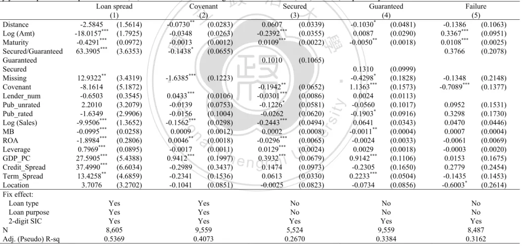
(35) regressions.3 Credit spread is the difference between BAA and AAA corporate boand yields. It tends to widen in recessions. Term spread is the difference between 10-year and 2-year Treasury yields. It tends to widen if economic prospects are good. Physical distance between borrower and lead bank may also influence loan contract terms (Giannetti and Yafeh, 2012), hence, I control location dummy variable which is equal to 1 if the borrower and lead bank have the same 3-digit zip code and 0 otherwise. Definitions of aforementioned variables are provided in Appendix B, Table B1. Finally, various fixed effects (2-digit SIC fixed effect, loan type fixed effect, or. 政治大 clustered at the year level throughout my analysis. 立. loan purpose fixed effect) are also controlled in the regressions. Standard errors are 4. ‧ 國. 學. 4. Data and Descriptive Statistics. Data on syndicated loans are collected from Reuters Loan Pricing Corporation. ‧. (LPC) DealScan database, which provides detailed information on contract terms,. sit. y. Nat. borrowers, and lenders. I focus on the U.S. market in the period from January 1990 to. io. er. August 2010. The initial data consists of 60,237 deals or 86,904 facilities.. al. n. Facilities with only one lender are excluded from the analyses because the physical and relational. i n C distance h cannot e n gbe ccalculated. hi U I. v. use lenders’ geographic. information to compute their physical distance. The cities of the lenders’ principal executive offices are used to calculate the average physical distance on the syndicated loan facility level between 1990 and 2010. I am able to identify the geographic data for 23,188 deals or 31,938 facilities (hereafter referred to as Sample I).. 3. My yearly GDP per capita data is from World Bank’s World Development Indicators. The credit. spread and term spread are monthly data and they are from Federal Reserve Board of Governors. 4. Results are stronger if standard errors are clustered at the borrower or the loan type level. I, therefore,. report the most conservative outcomes. 21.

(36) The information of lenders’ roles (leader or participant) is used to construct the syndication networks between 1990 and 2009. Because the networks are not static, following previous literature, I use overlapping, moving five-year windows to construct collaboration networks amongst lenders (Baum et al., 2004, Hochberg et al., 2007, 2010, and Godlewski et al., 2012). Sixteen moving windows (i.e. sixteen networks) are used to compute the relational distance for the members of each facility from 1995 to 2010. There are 44,327 deals or 65,390 facilities in this sample (hereafter referred to as Sample II).. 政治大 2.1 shows that the average loan size is 172 (265) million with a 223 (227) bps spread 立 Descriptive statistics of the variables are provided in Table 2.1. Panel A of Table. over LIBOR rate for sample I (sample II). While the mean (median) of loan amount is. ‧ 國. 學. larger in Sample I than in Sample II, the mean (median) spreads are similar for both. ‧. samples. The fraction of secured loans is high in both samples. For Sample I, 82% of. y. Nat. the loans are secured. In contrast, 78% of the loans are secured for Sample II. Due to. er. io. sit. the fact that there are many missing values for the variable Secured in the DealScan database, I treat these missing values as unsecured facility throughout my analyses,. al. n. v i n C his a dependent variable. except in the case when Secured My treatment of missing engchi U values as unsecured facility clearly may give rise to a bias estimate on the coefficient of the Secured variable. To ameliorate the effect of this bias, I define a dummy variable that takes the value one if the variable Secured is missing, and zero otherwise, and I include this variable in my regression to control for the effect of my treatment on the missing values. [Insert Table 2.1] The cases of syndication failures consist of 0.6% (0.5%) of the total observations in Sample I (Sample II). The borrowers are divided into three types: private, public 22.

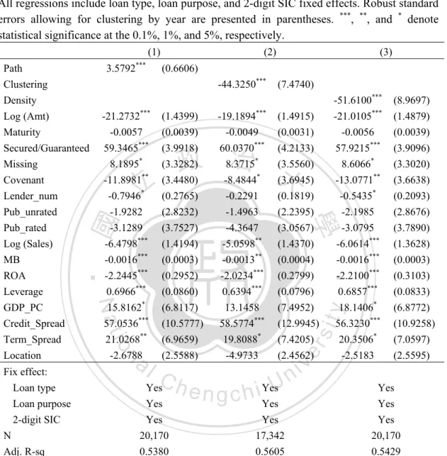
(37) and unrated, and public and rated. They are used as proxies for the borrowers’ informational opacity (Sufi, 2007, 2009; Dennis and Mullineaux, 2000; Lee and Mullineaux, 2004; Bosch and Steffen, 2011). I match my sample with Compustat to obtain borrowers’ financial variables and their descriptive statistics are shown in Panel B. The average firm size in terms of sales is about 3.2 billion in Sample I and about 4.9 billion in Sample II. There are more missing values for the market to book value (MB) ratio than other financial variables. I am able to retrieve 11,359 (24,742) observations of MB ratio in Sample I (Sample II).. 政治大 between any two lenders is 2,571 kilometers and the standard deviation is 2,433. In 立 Panel C reports the four distance measures. The average physical distance. the formal analysis, I standardize the physical distance to facilitate the interpretation. ‧ 國. 學. and expression of the regression coefficient. The mean of the average path length is. ‧. 1.68 which is much smaller than 6.9, the average lender number. The means of the. sit. y. Nat. clustering coefficient and density are 0.84 and 0.79, respectively.. n. al. er. io. 5. Empirical Results. 5.1. Results for Physical Distance. Ch. engchi. i n U. v. I first examine my hypotheses using physical distance as the proxy for segmented communication amongst lenders. The regression results are reported in Table 2.2. It is seen from column (1) that the coefficient of physical distance is -2.58. The sign is inconsistent with my model’s prediction although it is statistically insignificant. The result should be interpreted with caution because physical distance is sensitive to the existence of foreign lenders. The presence of foreign lenders in a facility will lengthen the physical distance, which can bias my results (Mian, 2006; Haselmann and Wachtel, 2011). When I divide my sample to those with and without foreign lender, and. re-run. the. regression,. the. coefficient 23. on. physical. distance. for.

(38) without-foreign-lender subsample become positive although it is still statistically insignificant.5 In columns (2) to (4), the relationship between physical distance and other non-price contract terms are either insignificant or of the wrong sign. When I divide my sample into those with and without foreign lender, the conclusion does not change. These results show that the effects of physical distance on syndicated loan contract terms are weak. In addition, column (5) shows that physical distance seems to lack explanatory power in predicting loan failures.. 立. [Insert Table 治 2.2] 政大. One possible reason that my model’s predictions are not supported by physical. ‧ 國. 學. distance may be that using lenders’ principal executive offices to calculate the distance is questionable. For example, if lending decision is made by banks’ branches,. ‧. my calculation of physical distance may be biased. To disentangle this concern, I. sit. y. Nat. assume that the lending decision is made by principal executive offices as loan size is. al. er. io. large, and it is made by branches as loan size is small. I, therefore, divide my sample. v. n. into large loans and small loans according to the sample median of the ratio of facility. Ch. engchi. i n U. amount to borrower’s total asset and re-run the regression. However, the pattern of the results is unchanged.6 In summary, none of my three hypotheses are supported if physical distance is used to proxy for segmentation of communication amongst lenders. The coefficients on control variables are mostly consistent with those reported in the literature. In column (1), loan spread tend to decrease with loan amount and maturity (e.g., Ivashina, 2009; Ivashina and Sun, 2010; Cai et al., 2010). The loan 5. The results are provided in Appendix B, Tables B2 and B3.. 6. The results are provided in Appendix B, Tables B4 and B5. 24.

(39) spreads on secured/guaranteed loans are significantly higher than those on unsecured/non-guaranteed loans (e.g., Focarelli et al., 2007; Ivashina, 2009; Nandy and Shao, 2010). The coefficient of the “missing” variable is positive and significant. This means I may have underestimated the coefficient of Secured/Guaranteed because I treat the missing value as unsecured/non-guaranteed. The results also show that macroeconomic factors and borrowers’ size, growth opportunity, profitability, and capital structure are all important determinants of loan spread. In column (2), the coefficients on control variables reveal some interesting. 政治大 negative effect on the existence of financial covenants. Somewhat surprisingly, the 立. patterns. The loan amount and the size of borrowers have a statistically significant and. coefficients on ROA and leverage are statistically significant but their signs are. ‧ 國. 學. different from those reported in column (1). Intuitively, if the borrower’s profitability. ‧. is high and leverage is low, then I would expect the financial covenants to be less. y. Nat. binding. My results suggest that borrowers who are less financially constrained are. er. io. sit. more likely to use financial covenants to attract potential lenders.. In column (5), I confine my analysis to data with lender numbers between two. al. v i n The coefficients of C the control variables U h e n g c h i indicate that the probability of n. 7. and ten.. syndication failure is higher with larger loan amount or longer maturity. Loans with. 7. As noted earlier, my model predicts that failures will concentrate more on loans with low number of. lenders. The frequency distributions reported in Table B6 of Appendix B support the prediction. In Table B6, the number of syndication failures decreases as the number of lenders increases. However, the number of failures is falling at a faster rate than the increase in observations thus giving rise to a falling proportion of failures. This is with the exception of lender numbers eight and nine for both samples. Given this pattern in lender number and syndication failures, when H3 are tested, I confine my analysis to data with lender numbers between two and ten. 25.

(40) financial covenants are less likely to fail. Borrowers’ financial characteristics seem to exert little influence on failure probability. 5.2. Results for Relational Distance Results in the previous section suggest that communication amongst lenders does not seem to be affected by physical distance. In this section, I consider another proxy for communication segmentation, the relational distance, and test its effect on syndicated loan contracts. 5.2.1. Relational distance and loan spreads. 政治大. First, I test the relationship between relational distance and loan spread. The. 立. regressions are performed using equation (6) to test hypothesis one. The results are. ‧ 國. 學. presented in Table 2.3. In all specifications, my proxies for relational distance have statistically significant effects on loan spreads. Column (1) shows that the coefficient. ‧. of average path length (Path) is positive and statistically significant at the 0.1% level.. Nat. sit. y. Columns (2) and (3) show that the coefficients of clustering coefficient (Clustering). n. al. er. io. and density (Density) are negative and statistically significant at the 0.1% level. These. i n U. v. results lend support to my hypothesis that the further the relational distance, the. Ch. engchi. higher is the probability of a cascade occurring, hence the larger is the spread. [Insert Table 2.3] The effect of relational distance on loan spreads is also economically significant. A one-standard deviation increase (decrease) in average path length (clustering coefficient/density) increases the all-in-drawn spread by 7.7 (11.5/15.0 ) basis points, which is approximately 3.4 (5.1/6.7) percent of the sample median spread of 225 basis points. The coefficients of the control variables are by and large similar to those reported in column (1) of Table 2.2. In column (1), loan spreads significantly decrease with 26.

(41) loan amount. The reason may be due to the effect of economies of scale (Graham et al., 2008; and Godlewski et al., 2012) or because larger borrowers, which have greater transparency and lower default risk, typically issue larger loans (Focarelli et al., 2008; and Carey and Nini, 2007). The negative coefficient on maturity seems to be consistent with ‘credit-quality hypothesis’ – banks limit their exposure by lending riskier borrowers shorter loans (see, for example, Gottesman and Roberts, 2004). The loan spreads on secured/guaranteed loans are significantly higher than those on unsecured/non-guaranteed loans. This result seems to support “observed-risk. 政治大 collateral (see, for example, Godlewski and Weill, 2011). The coefficient of the 立 hypothesis” – banks charge riskier borrowers larger loan spreads and require more. “missing” variable is positive and significant. This means I may have underestimated. ‧ 國. 學. the coefficient of Secured/Guaranteed because I treat the missing value as. ‧. unsecured/non-guaranteed.. y. Nat. Loans with financial covenants seem to have lower spreads. The intuition may be. er. io. sit. that covenants is a contract design that can work as an ex ante monitoring device to moderate moral hazard, which in turn reduces the loan spread (Ivashina, 2009).. n. al. Ch. n U engchi. iv. Lee. and Mullineaux (2004) and Bosch and Steffen (2011) showed that syndicate size is larger when the borrower has higher transparency and lower credit risk. This finding is consistent with my negative coefficient on lender number. I also find that borrowers’ characteristics such as larger size, higher growth opportunities, and greater profitability are negatively associated with loan spreads. Borrowers with higher leverage bear higher loan spreads. GDP per capita and credit spread have significant influence on loan spread, which is consistent with the findings of Giannetti and Yafeh (2012) and Graham et al. (2008).. 27.

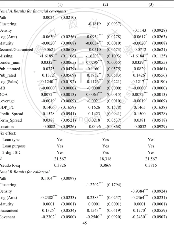
(42) 5.2.2. Relational distance and non-price requirements In this section, I run probit regressions to test my second hypothesis. The results are presented in Table 2.4. In Panel A of Table 2.4, I examine whether the probability of setting financial covenants increases with relational distance measures. The results show that the coefficients of my variables of interest, Path, Clustering, and Density, are statistically insignificant at conventional levels of significance. Relational distance does not seem to exert any influence on the probability of having financial covenants. As for the coefficients of the control variables, they are qualitatively the same as those reported in column (2) of Table 2.2. Again I find that financially less constrained. 政治大. firms typically characterised by higher ROA and lower leverage are more likely to use. 立. [Insert Table 2.4]. 學. ‧ 國. financial covenants.. ‧. Panel B of Table 2.4 reports the regression results for collateral requirements. In. sit. y. Nat. column (1), the coefficient of average path length is positive and statistically. io. er. significant with a value of 0.11. In columns (2) and (3) the coefficients of the clustering coefficient and density are negative and statistically significant at the 1%. al. n. v i n level. These results suggest thatCthe hlonger i U distance amongst lenders, e n giscthehrelational the higher is the probability of requiring collateral, which is consistent with hypothesis two. In addition, the coefficients of the control variables show that loans. with higher amount are less likely to require collateral. The probability of requiring collateral is lower for public firms than for private firms. Large sized borrowers tend to have lower probability of offering collateral. Unlike the results for financial covenants, there is evidence to suggest that borrowers that are more financially constrained, as characterised by lower profitability and higher leverage, are more. 28.