基於多級樹狀結構之球狀解碼器實現

全文

(1)國立交通大學電機與控制工程研究所碩士論文. 基於多級樹狀結構之球狀解碼器實現 Implementation of K-Best sphere decoder based on multistage tree structure. 指導教授：董蘭榮. 博士. 研究生：黃致惟. 中華民國九十六年九月.

(2) Implementation of K-Best sphere decoder based on multistage tree structure. Advisor: Dr. Lan-Rong Dung Graduate Student: Zhi-Wei Huang. September 2007. Graduate Institute of Electrical and Control Engineering National Chiao Tung University Hsinchu, Taiwan, ROC.

(3) 基於多級樹狀結構之球狀解碼器實現. 學生：黃致惟. 指導教授：董蘭榮. 博士. 國立交通大學電機與控制工程學系研究所. 摘要. 在多重輸入輸出(MIMO)的通訊系統中，最大概似(ML)偵測具有相當突出的性能表現。但是最大概似偵測的主要缺點在於計算複雜度隨著天線數量與調變階數的遞增而指數增加。因此我們考慮以樹狀搜尋為基礎的 K-Best 演算法。 K-Best 演算法的效能接近最大概似偵測，但計算複雜度卻比最大概似偵測低。本篇論文提出了多級 K-Best 演算法應用在多重輸入輸出系統。在所提出的方法中，主要是將高階星狀點分解成許多低階星狀點，並且應用有順序性地偵測低階星狀點的技巧來降低最大概似解錯失的機率。實驗結果發現多級 K-Best 演算法相較於傳統 K-Best 演算法不僅擁有較低的計算複雜度同時也能夠達到幾乎相同的效能。同時在本篇論文的最後也以目前數位積體電路技術來實現多級 K-Best 偵測器的架構。. i.

(4) Implementation of K-Best sphere decoder based on multistage tree structure. Graduate Student: Zhi-Wei Huang. Advisor: Dr. Lan-Rong Dung. Department of Electrical and Control Engineering National Chiao Tung University. Abstract. In multiple-input multiple-output (MIMO) communication systems MaximumLikelihood detection is the preferred detection method which achieves the optimal performance. However, the main drawback of Maximum-Likelihood detection is that it suffers from exponential computational complexity against the number of antennas and signal modulation methods. Thus we consider K-Best algorithm based on the breadth-first tree search. The K-Best algorithm provides near-ML performance while its computational complexity is reduced compared to the Maximum-Likelihood detection. This thesis proposes the multistage K-Best algorithm in MIMO systems. In the proposed method, we decompose higher order constellation into several lower order constellations and apply ordering of lower order constellation to reduce the probability of missing the Maximum-Likelihood solution. It can be seen that the multistage K-Best algorithm and conventional K-Best algorithm achieve almost identical PER performance at the same K value. However, the multistage K-Best algorithm is shown to achieve such performance with a significantly lower computational complexity compared to the conventional K-Best algorithm. At the same time the VLSI architecture for the implementation of the multistage K-Best algorithm based on 0.18-μm technology is presented. ii.

(5) 誌謝首先我要感謝指導教授董蘭榮教授，在論文研究與求學態度上給予詳盡且細心的指導，再來要感謝系統晶片實驗室的學長與同學們的幫忙，最後我要感謝我的家人以及一直在我身邊的好朋友們，給我最大的精神鼓勵與支持。. iii.

(6) Contents Abstract in Chinese .........................................................................................................i Abstract in English.........................................................................................................ii Contents ........................................................................................................................iv List of Tables................................................................................................................vii List of Figures ............................................................................................................ viii. Chapter 1. Introduction ..........................................................1. 1.1 Motivation........................................................................................................2 1.2 Organization Of This Thesis ............................................................................3. Chapter 2. Backgrounds..........................................................4. 2.1 Detection Methods Overview ..........................................................................4 2.1.1 MIMO System Model ...........................................................................4 2.1.2 Zero-Forcing .........................................................................................6 2.1.3 Minimum Mean-Squared Error.............................................................7 2.1.4 Ordered Successive Interference Cancellation .....................................8 2.1.4.1 Zero-Forcing Nulling .................................................................9 2.1.4.2 Minimum Mean-Squared Error Nulling ..................................10 2.1.5 Sphere Decode ....................................................................................11 2.1.5.1 Real-Valued System Model .....................................................11 2.1.5.2 Sphere Decode Algorithm........................................................12 2.1.6 Maximum-Likelihood .........................................................................15 iv.

(7) 2.2 QR-Decomposition Overview .......................................................................17 2.3 CORDIC Overview........................................................................................19. Chapter 3 MIMO Detection By Tree Search ...................... 24 3.1 Principles Of Tree Search Algorithm.............................................................24 3.1.1 Breadth-First Tree Search ...................................................................26 3.1.2 Depth-First Tree Search......................................................................28 3.2 Proposed Signal Detection Scheme ...............................................................29 3.2.1 Multistage K-Best Algorithm .............................................................29 3.2.2 Ordering of Lower Order Constellation..............................................35 3.2.3 Complexity Analysis...........................................................................37. Chapter 4 Simulation Result................................................ 40 4.1 Platform Description......................................................................................40 4.2 Performance Evaluation.................................................................................43. Chapter 5. Hardware Architecture ...................................... 47. 5.1 QR-Decomposition Architecture ...................................................................48 5.1.1 Triangular Systolic Array ...................................................................48 5.2 Matrix-Vector Multiplication Architecture....................................................51 5.3 Multistage K-Best Detection Architecture.....................................................52 5.3.1 Sorting Network..................................................................................54 5.3.1.1 Bubble-Sort ..............................................................................56 5.3.1.2 Batcher’s Bitonic-Sort .............................................................56. v.

(8) 5.3.1.3 M. Afghahi’s Sort.....................................................................57 5.3.1.4 Linear-Sort ...............................................................................58 5.3.2 Metric Calculation Unit ......................................................................59 5.4 Experiment Reports for Hardware Implementation.......................................61 5.4.1 The Area And Power Estimation ........................................................61. Chapter 6. Conclusion ........................................................... 64. 6.1 Conclusion .....................................................................................................64 6.2 Comparison ....................................................................................................65 6.3 Future Work ...................................................................................................66. References................................................................................. 67. vi.

(9) List of Tables. [Table 2-1]. Function of the CORDIC in the different modes of operation ......20. [Table 5-1]. Area report for each unit and component.......................................62. [Table 6-1]. Comparison of implementation results ..........................................65. vii.

(10) List of Figures [Figure 2-1] Block diagram of the MIMO system..............................................5 [Figure 2-2] CORDIC Processor ......................................................................21 [Figure 2-3] Unrolling CORDIC Structure.......................................................22 [Figure 3-1] Flowchart of multistage K-Best algorithm ...................................32 [Figure 3-2] Example of multistage K-Best algorithm represented in tree form ......................................................................................................34 [Figure 3-3] Total computational complexity comparison for 64-QAM MIMO system with four transmit and four receive antennas ...................38 [Figure 3-4] Reduction in computational complexity for 64-QAM MIMO system with four transmit and four receive antennas ...................38 [Figure 3-5] Total computational complexity comparison for 64-QAM MIMO system with two transmit and two receive antennas ....................39 [Figure 3-6] Reduction in computational complexity for 64-QAM MIMO system with two transmit and two receive antennas.....................39 [Figure 4-1] MIMO-OFDM Transmit Scheme.................................................42 [Figure 4-2] MIMO-OFDM Receive Scheme ..................................................42 [Figure 4-3] The PER for MR = MT = 2 with 64-QAM and coding rate 2/3 ....45 [Figure 4-4] The PER for MR = MT = 2 with 64-QAM and coding rate 3/4 ....45 [Figure 4-5] The PER for MR = MT = 4 with 64-QAM and coding rate 2/3 ....46 [Figure 4-6] The PER for MR = MT = 4 with 64-QAM and coding rate 3/4 ....46 [Figure 5-1] Block diagram of MIMO detector................................................47 [Figure 5-2] Block diagram of Triangular Systolic Array ................................50 [Figure 5-3] Hardware realization of the matrix-vector multiplication array...51 viii.

(11) [Figure 5-4] Pipeline architecture for multistage K-Best detection..................53 [Figure 5-5] Hardware architecture of each layer.............................................53 [Figure 5-6] Bubble-sorting network for 16 inputs...........................................54 [Figure 5-7] Batcher’s bitonic-sorting network with I/O size 16 .....................55 [Figure 5-8] Block diagram of M. Afghahi’s sorting network..........................55 [Figure 5-9] Number of comparators in the different sorting network for various N.....................................................................................57 [Figure 5-10]. Block diagram of linear-sorting network ...................................58. [Figure 5-11]. Architecture of metric calculation unit at the first stage ............60. [Figure 5-12]. Architecture of metric calculation unit at the ith stage (2≤ i ≤q) ..60. [Figure 5-13] Chip layout by SOC Encounter ..................................................63 [Figure 6-1] Block diagram of an iterative receiver .........................................66. ix.

(12) Chapter 1. Introduction. Due to the spectral efficiency achievable near Shannon capacity limit [1], multiple-input multiple-output (MIMO) systems with multiple antennas at both transmitter and receiver that realize a high bit rate data transmission have drawn much attention in the wireless communication area recently [2] [3]. Orthogonal Frequency Division Multiplexing (OFDM) [4] is a multicarrier transmission technique. The basic principle of OFDM is to split the available bandwidth into many narrow band channels. The carriers for each channel are made orthogonal to one another. This results in OFDM system having lower rate parallel subcarriers. Because the symbol duration increases resulted from lower rate datastreams, the dispersion caused by multipath delay spread is reduced. The benefits of OFDM are superior tolerance to multipath fading, high spectral efficiency, achieving high data rate, and increasing the robustness against narrowband interference. Therefore, combining MIMO with OFDM technology (MIMO-OFDM) [5] holds great promise for wide use in next-generation wireless communication systems.. 1.

(13) 1.1 Motivation Several signal detection algorithms for higher data rate in MIMO systems had been proposed [6] [7]. It is known that the optimal Maximum-Likelihood algorithm has much better performance. Unfortunately, it is usually infeasible for hardware implementation because the complexity increases exponentially with the number of antennas and symbol alphabet. On the other hand, although simple detection algorithms are suitable implemented, their performances are often unsatisfactory. Consequently, there are enormous researches on low complexity near-optimal methods when higher order constellations and large number of antennas are applied [8] [9] [10]. Efficient algorithms such as sphere decode algorithm which achieves ML or near-ML performance and reduces detection complexity have been widely considered for MIMO systems [11] ~ [18]. VLSI implementation of sphere decode algorithm has been studied in several papers [19] [20] [21]. At the same time a careful study of the VLSI implementation aspect is also important to achieve economic MIMO detection implementations. In this thesis, we propose algorithm-level and VLSI architecture of multistage K-Best detection scheme to tackle the implementation challenge of the conventional K-Best detection scheme for higher order constellation such as 64-QAM over MIMO channels. The basic idea is to reduce the total number of candidates in the multistage K-Best algorithm. For the reason, the computational complexity is reduction.. 2.

(14) 1.2 Organization Of This Thesis This thesis is organized as follows. In Chapter 2, we briefly review the conventional signal detection algorithms, Zero-Forcing, Minimum-Mean-SquaredError, Ordered-Successive-Interference-Cancellation, Sphere-Decode and MaximumLikelihood. Chapter 3 presents the concept of QR-decomposition based tree search algorithm and describes the practical problems of implementing conventional K-Best detector. Then we introduce the proposed detection scheme that is multistage K-Best detection scheme. In Chapter 4, the MIMO-OFDM system model is described. The proposed algorithm is applied to the system and its performance is evaluated through computer simulations. A comparison between the conventional K-Best algorithm and multistage K-Best algorithm is also provided. Chapter 5 explains the VLSI architecture of the multistage K-Best detector. Finally, the conclusion and future work are given in Chapter 6.. 3.

(15) Chapter 2. Backgrounds. 2.1 Detection Methods Overview 2.1.1 MIMO System Model We consider the MIMO system with a transmit array of MT antennas and a receive array of MR antennas. The single data stream in the input is demultiplexed into MT substreams, and each substream is modulated independently then transmitted by its dedicated antenna. Throughout the thesis, we focus on the case MR ≥ MT. The block diagram of a MIMO system is shown in Figure 2-1. The channel is assumed to be a Rayleigh fading channel and it is quasi-static. Since channel matrix can be estimated at the receiver by transmitting a training sequence, we assume that the channel matrix is known perfectly to the receiver. The equivalent complex valued baseband system model for the MIMO channel is as follows : ~ ~ ~ y = H ~s + n. (2.1). ~ where received vector ~ y is the MR×1 column matrix, H is the MR×MT complex channel matrix, whose component ~h i, j is the fading coefficient from the jth transmit antenna to the ith receive antenna, transmitted symbol vector ~s is the MT×1 column ~. matrix, whose entries are chosen independently from some complex constellation O 4.

(16) ~ is a MR×1 column matrix, with k bits per constellation symbol, noise vector n whose elements are independent identically distributed (i.i.d.) circularly symmetrical complex Gaussian variables. The reality of MIMO receivers is that we need to contend with multistream interference, since the transmitted streams are not truly independent and they interfere with each other. In addition to this, we have the problem of channel fading and additive noise. The main goal of this section is to review different methods for detection. The five most common detections are Zero-Forcing, Minimum-MeanSquared-Error, Ordered-Successive-Interference-Cancellation, Sphere-Decode and Maximum-Likelihood. We shall now briefly examine these.. [Figure 2-1] Block diagram of the MIMO system. 5.

(17) 2.1.2 Zero-Forcing The Zero-Forcing equalizer uses an inverse filter to compensate for the channel response function. It behaves like a linear filter that does not consider the effects of noise. In fact, the noise may be enhanced in the process of eliminating the interference.. ~ Let us assume the case that MR = MT and H is a full rank square matrix. In this ~ case, the inverse of the channel matrix H exists. Multiplying both sides of (2.1) by. ~ H−1 results in ~ ~ ~ H −1 ~ y = ~s + H −1 n. (2.2). and we can estimate the transmitted data symbol vector as ~ −1 ~ ~sˆ = H y ZF. (2.3). The symbols can be decoded by finding the closest constellation point to the element ~ ~ ~ of H −1 ~ may be more than the power of y . However, the power of the noise H−1 n ~ ~ . The noise enhancing factor for a given channel matrix H the original noise n can be calculated as ~ ~ ~ ~ (H −1 ) H (H −1 ) = (H H H ) −1. (2.4). where the superscript ” H “ denotes the complex conjugate transpose. Therefore, the ~ ~ noise power may increase because of the factor (H H H ) −1 .. ~ ~ ~ ~ ~ If MR > MT and H is a full rank, we have H † = (H H H) −1 H H where † represents pseudo inverse. Therefore, we may multiply (2.1) by the pseudo inverse of. ~ H , we have. 6.

(18) ~ ~ ~ H† ~ y = ~s + H † n. (2.5). and estimate the transmitted data symbol vector as ~sˆ. ZF. ~ = H† ~ y. (2.6). ~ ~ ~ Note that if H is square and non-singular, we have H † = H -1 and achieve the same results as before. Separate decoding of the symbols is possible by finding the closest ~ constellation point to the element of H † ~ y . The noise enhancing factor is. ~ ~ ~ ~ ~ ~ ~ ~ ~ ~ (H † ) H (H † ) = [(H H H) −1 H H ]H [(H H H) −1 H H ] = (H H H ) −1. (2.7). In general, the Zero-Forcing approximation does not coincide with the MaximumLikelihood solution and hence it is not optimal.. 2.1.3 Minimum Mean-Squared Error ~ Another linear detection algorithm is to choose a matrix Q that minimizes the. mean square error : ε 2 = E [( ~s − ~sˆMMSE ) H ( ~s − ~sˆMMSE )]. (2.8). The goal of the linear MMSE equalizer is to multiply (2.1) by a matrix such that the resulting effective noise is minimized. Unlike the Zero-Forcing method, the ~ received vector is multiplied by a matrix Q that is a function of SNR. The matrix ~ Q is equal to : −1. ~ ⎛ I MR ~ ~⎞ ~ Q = ⎜⎜ + H H H ⎟⎟ H H ⎝ SNR ⎠. 7. (2.9).

(19) Therefore, the resulting MMSE estimate of ~s is : ~sˆ. MMSE. −1. ⎛ I MR ~ ~ ~⎞ ~ = Q×~ + H H H ⎟⎟ H H × ~ y = ⎜⎜ y ⎝ SNR ⎠. (2.10). The MMSE technique can provide somewhat better estimates of ~s than the Zero-Forcing algorithm, at a similar computational cost. However, the evaluation of the MMSE solution requires knowledge of the ratio IMR / SNR. The above linear equalization methods are based on multiplying the received vector by a matrix and then decoding the symbols separately.. 2.1.4 Ordered Successive Interference Cancellation Rather than jointly decoding all symbols, ordered successive interference cancellation algorithm first decodes the strongest symbol. Then, canceling the effects of this strongest symbol from all received signals, the algorithm detects the next strongest symbol. The algorithm continues by canceling the effects of the detected symbol and the decoding of the next strongest symbol until all symbols are detected. The ordered successive interference cancellation algorithm has better performance than MMSE, ZF but suffers from error propagation. Therefore, ordered successive interference cancellation algorithm is still suboptimal. Representing the ith symbol of the transmitted vector ~s by ~s i and the ith. ~ ~ column of channel matrix H by Hi , (2.1) can be written as ~ y =. MT. ~ ~ ~ i si + n. ∑H i =1. (2.11). The ordered successive interference cancellation algorithm is as follows: • Ordering: When symbol cancellation is used, the order in which the symbols are detected will impact the overall performance of the system. Therefore, the optimal 8.

(20) detection order is from the strongest symbol (highest SNR) to the weakest one (lowest SNR). Note that changing the order of the symbols in transmitted vector ~s. ~ will not change (2.11) if the order of the columns of channel matrix H changes accordingly. • Cancellation: The goal of the cancellation is to cancel the effect of the detected signal from the received signal vector to reduce the detection complexity for the remaining signals. • Nulling: Interference nulling can be considered as removing the effects caused by undetected symbols from the one that is being decoded. The specifics of the detection process depend on the criterion chosen to compute the nulling vectors. There are many different methods to detect a symbol. The most common choices of these methods are Zero - Forcing and Minimum mean - squared error. We describe these two methods separately.. 2.1.4.1 Zero-Forcing Nulling Symbols ~s 1 , ~s 2 , L , ~s i-1 have been already detected at stage i of the algorithm. Let us assume a perfect decoder that is the decoded symbols ~sˆ 1 , ~sˆ 2 , L , ~sˆ i -1 are the same as the transmitted symbols ~s 1 , ~s 2 , L , ~s i-1 . The effects of ~s 1 , ~s 2 , L , ~s i-1 have been canceled and the remaining undetected symbols to the received vector is as follows : ~y = ~ y − i. i −1. ∑. j =1. ~ H j ~s j =. MT. ~ ~ ~ j sj + n. ∑H j= i. i = 2 ,3 , L M T − 1. (2.12). Therefore, to decode ~sˆ i , first we should calculate Mi. The ith row of Z†, denoted by Mi is the Zero-Forcing nulling vector with the minimum norm for the ith symbol, where Z† denotes the pseudo - inverse of Z, Z denotes the matrix obtained by 9.

(21) ~ zeroing columns 1 , 2 , … , i−1 of H . Mi is orthogonal to interference vectors ~ ~ ~ ~ H i+1 , H i+ 2 , L , H M T but not orthogonal to Hi . We can use the formula in (2.12) and ~ the character of Mi to separate the term H i ~s i from ~y i . Then, We have ~ M i ~y i = ~s i + M i n. (2.13). The decoded symbol ~sˆ i is the closest constellation point to M i ~y i . Assuming that ~sˆ i = ~s i , cancel ~s i from the received vector ~y i ; the modified received vector ~y : i+1. ~ ~ y i+1 = ~y i − H i ~s i. (2.14). ~ ~ where Hi denotes the ith column of H . The ordered successive interference cancellation combined with the ZF algorithm continues recursively until all symbols are detected.. 2.1.4.2. Minimum Mean-Squared Error Nulling. In the ith stage of ordered successive interference cancellation algorithm, the effects of ~s 1 , ~s 2 , L , ~s i-1 have been removed. Therefore, to find ~sˆ i , first we should. ~ replace H in (2.9) with Z as we did in the Zero-Forcing case. −1. ⎛ IMR ⎞ W = ⎜⎜ + Z H Z ⎟⎟ Z H ⎝ SNR ⎠. (2.15). The ith row of W, denoted by Wi is the MMSE nulling vector with the minimum ~ ~ ~ norm for the ith symbol. Wi is orthogonal to interference vectors H i +1 , H i + 2 , L , H M. T. ~ but not orthogonal to Hi . We can use the character of Wi and multiply Wi by the. vector ~y i. 10.

(22) ~ W i ~y i = ~s i + W i n. (2.16). The best estimate of the ith symbol ~sˆ i is the closest constellation point to W i ~y i . Assuming that ~sˆ i = ~s i , cancel ~s i from the received vector ~y i ; the. modified received vector ~y i+1 : ~ ~ y i+1 = ~y i − H i ~s i. (2.17). ~ ~ where Hi denotes the ith column of H . The ordered successive interference cancellation combined with the MMSE algorithm continues recursively until all symbols are detected. The MMSE receiver suppresses both the interference and noise components, whereas the ZF receiver removes only the interference components. Therefore, the ordered successive interference cancellation combined with the MMSE algorithm is superior to the ordered successive interference cancellation combined with the ZF algorithm.. 2.1.5 Sphere Decode 2.1.5.1 Real-Valued System Model A solution for QAM constellations is frequently to decompose the MT dimensional complex signal model in (2.1) into a 2MT dimensional real-valued problem, i.e., real and imaginary parts of the received vector can be detected independently of each other. The corresponding real-valued input and output relation is as follows :. { H~ } − ℑ{ H~ }⎤ ⎡ℜ{ ~s }⎤ + ⎡ℜ{ n~ }⎤ { H~ } ℜ{ H~ } ⎥⎦ ⎢⎣ℑ{ ~s }⎥⎦ ⎢⎣ℑ{ n~ }⎥⎦. y }⎤ ⎡ℜ ⎡ℜ{ ~ ⎢ ℑ{ ~ ⎥=⎢ ⎣ y }⎦ ⎣ ℑ. 11. (2.18).

(23) where ℜ{•} and ℑ{•} denote the real and imaginary part of {•} respectively. The above equation includes only real - valued numbers and can be written in terms of real-valued matrices as y=Hs+n. (2.19). where s is a real - valued vector whose elements belong to a finite alphabet Ο . The ~. constellation Ο is separable into two constellations Ο for the real and imaginary parts of the symbols respectively. This approach can reduce the complexity of Partial Euclidean Distance (PED) calculation, since the number of children per node becomes smaller. The drawback of real-valued operation is that the tree is twice as deep as that of complex-valued operation.. 2.1.5.2. Sphere Decode Algorithm. To have the transmitted signal far from the received signal, the instantaneous power of the noise should be large. A larger instantaneous power of the noise is less likely than a smaller one because of the white Gaussian nature of the noise. Therefore, intuitively, it is more likely to have the most likely codeword in a neighborhood close to the received signal. The main idea of sphere decoding is to limit the number of possible codewords by considering only those codewords that are within a sphere centered at the received vector. Therefore, the overall complexity of the sphere decoding is lower than the full search ML decoding that requires an exponential complexity. In the follows, we consider sphere decoding and describe the technique in its simplest version. We say that a vector s (whose elements belong to constellation Ο ) lies in a 12.

(24) sphere with radius r if it approximates the solution with a residual norm less than r : ∥y − H s∥2 < r 2. (2.20). Let ŝZF = ( H H H )－1 H H y be the Zero-Forcing solution. It follows that ∥H ( s − ŝZF )∥2. =∥H s∥2 +∥H ŝZF∥2 − 2 ⋅ ŝZFH H H H s =∥H s∥2 +∥H ŝZF∥2 − 2 ⋅ y H H ( H H H )－1 H H H s =∥H s∥2 +∥H ŝZF∥2 − 2 ⋅ y H H s =∥y − H s∥2 −∥y∥2 +∥H ŝZF∥2. (2.21). and consequently ∥R ( s − ŝZF )∥2 =∥y − H s∥2 −∥y∥2 +∥R ŝZF∥2. (2.22). where R is the upper triangular matrix that is obtained via the QR-decomposition of the channel matrix H. It follows that a vector s lies in a sphere with radius r if and only if ∥R ( s − ŝZF )∥2 < r 2 −∥y∥2 +∥R ŝZF∥2. (2.23). The main idea behind the sphere decoding algorithm is described in the following way. Let r n2 = r 2 −∥y∥2 +∥R ŝZF∥2 where n is the length of s .Since R is an upper - triangular matrix :. 13. (2.24).

(25) ∥R ( s − ŝZF )∥2 n. =. ∑R k =1. 2 k ,k. ( sk − ŝZF(k) +. n. R k ,i. ∑R. i = k +1. ( si − ŝZF(i) ) ) 2. (2.25). k ,k. 2 2 = R n ,n ( sn − ŝZF(n) ) 2 + R n −1,n −1 ( sn−1 − ŝZF(n−1) +. R n −1,n R n −1,n −1. ( sn − ŝZF(n) ) ) 2 + …. ( here sk is the kth element of s , ŝZF(k) is the kth element of ŝZF ). From (2.25) it follows that a necessary condition for s to lie in a sphere with radius r is that R n2 ,n ( sn − ŝZF(n) ) 2 ≤ rn2. (2.26). or equivalently that ⎡ ŝZF(n) −. rn r ⎤ ≤ sn ≤ ⎣ ŝZF(n) + n ⎦ R n,n R n,n. (2.27). where ⎡ α ⎤ is the smallest integer greater than α and ⎣ α ⎦ is the greatest integer smaller than α. For a given sn ∈ s that satisfies (2.27) , let us define (2.28). rn2−1 = rn2 − R n2 , n ( sn − ŝZF(n) ) 2. ŝZF(n-1|n) = ŝZF(n-1) −. R n −1,n R n −1,n −1. ( sn − ŝZF(n) ). (2.29). Then a further necessary condition for s to lie in the sphere is : ⎡ ŝZF(n-1|n) −. rn −1 R n −1,n −1. ⎤ ≤ sn-1 ≤ ⎣ ŝZF(n-1|n) +. 14. rn −1 R n −1,n −1. ⎦. (2.30).

(26) For given sn ∈ s and sn-1 ∈ s in the intervals specified by (2.30) we can continue to obtain a bound on sn-2 that must be satisfied for s to lie in the sphere of radius r : ⎡ ŝZF(n-2|n-1) −. rn −2 R n − 2, n − 2. ⎤ ≤ sn-2 ≤ ⎣ ŝZF(n-2|n-1) +. rn −2 R n − 2, n − 2. ⎦. (2.31). where rn2− 2 = rn2−1 − R n2 −1, n −1 ( sn-1 − ŝZF(n-1|n) ) 2. ŝZF(n-2|n-1) = ŝZF(n-2) −. R n − 2,n −1 R n − 2, n − 2. ( sn-1 − ŝZF(n-1|n) ). (2.32). (2.33). The sphere decoding algorithm continues recursively to calculate the limits of the possible indices inside the sphere for each received vector. Then, among all possible codewords inside the sphere, it finds the closest codeword to the received vector. Note that the limits for the elements of the codeword depend on the choice of the radius r. For a very small value of r, it is possible that the sphere does not contain any point. In this case, either the decoder reports an error or it increases the value of r and repeats the process. On the other hand, a large value of r results in a huge number of possibilities and a slow decoding process. In practice, the value of r may be selected according to the SNR or may be adjusted adaptively.. 2.1.6 Maximum-Likelihood ML is an optimum receiver. Let us assume for the sake of simplicity that the data stream is temporally uncoded, The Maximum-Likelihood receiver solves ~ ~sˆ = arg min ~ y − H ~s ~ MT s ∈ο. where ~sˆ is the estimated symbol vector 15. 2. (2.34).

(27) The ML receiver searches through all the vector constellation for the most probable transmitted signal vector. If the modulation utilizes a constellation with 2k points to transmit k bits, the number of possibilities for codeword is 2Nk . For four transmit antennas and 16-QAM, k = 4, there are 65536 possibilities. Hence, ML receiver is difficult to implement, but provide full MR diversity and zero power losses as a consequence of the detection process. In this sense it is optimal.. 16.

(28) 2.2 QR-Decomposition Overview There are many methods such as LU-decomposition and QR-decomposition to triangularize a matrix. QR-decomposition (QRD) by Givens rotations which have been proven to be unconditionally stable for all nonsingular input matrices is a well-established technique [22]. This technique uses successive plane rotations to input matrix elements below the main diagonal to reduce the input matrix to an upper triangular matrix and forms the product of all plane rotations in order to construct a unitary matrix. Let review the Givens Rotation for the QR-decomposition of a n × n real matrix. The n × n real matrix B n × n is defined by：. ⎡ b 1 ,1 ⎢ b ⎢ 2 ,1 Bn × n = ⎢ M ⎢ ⎢ b n−1 ,1 ⎢ b n ,1 ⎣. b1, 2. L. b 1 , n−1. b 2 ,2 M. L O. b 2 , n−1 M. b n−1 , 2. L. b n−1 , n−1. b n ,2. L. b n , n−1. b1,n ⎤ b 2 , n ⎥⎥ M ⎥ ⎥ b n−1 , n ⎥ b n , n ⎥⎦. (2.35). To set to zero the matrix element below the main diagonal, we would have to multiply B n × n successively by Q∗1, 2 , L, Q∗1, n , L , Q∗ n −2 , n −1 , Q∗ n −2 , n , Q∗ n −1, n in the order. We multiply matrix B n × n from the left by a matrix Q∗1, 2 to annihilate the matrix element located at the first column and second row first. Then we multiply matrix Q∗1, 2 B from the left by a matrix Q∗1, 3 to annihilate the matrix element located at the third row and first column, etc. After such successive multiplications we are left with an upper triangular matrix R, namely,. Q∗B = R Q ∗ = Q ∗ n −1 , n Q ∗ n − 2 , n Q ∗ n − 2 , n −1 L Q ∗ 1 , n Q ∗ 1 , 3 Q ∗ 1 , 2 17. (2.36).

(29) Left multiplication of the matrix B n × n by matrix Q∗ i , j is equivalent to a micro plane rotation, where Q∗ i , j is the Givens’ rotation operator used to annihilate the matrix element located at ith column and jth row. The idea of micro plane rotation can be easily illustrated on the example of 4 × 4 real matrix and the product of all micro plane is defined by :. Q ∗ = Q ∗3,4 × Q ∗2,4 × Q ∗2,3 × Q ∗1,4 × Q ∗1,3 × Q ∗1,2 ⎡1 ⎢0 =⎢ ⎢0 ⎢ ⎣0. 0. 0. 1 0. 0 c 3,4 − s3,4. 0. ⎡ c 1,4 ⎢ 0 ⎢ ⎢ 0 ⎢ ⎣ − s1,4. 0 1 0 0. 0 ⎤ ⎡1 0 ⎥ ⎢ 0 ⎥ ⎢ 0 c 2,4 × s3,4 ⎥ ⎢0 0 ⎥ ⎢ c 3,4 ⎦ ⎣ 0 − s 2,4 0 s1,4 ⎤ ⎡ c 1,3 0 0 ⎥⎥ ⎢ 0 ×⎢ 1 0 ⎥ ⎢ − s1,3 ⎥ ⎢ 0 c 1,4 ⎦ ⎣ 0. 0. 0 ⎤ ⎡1 s 2,4 ⎥⎥ ⎢0 ×⎢ 0 ⎥ ⎢0 ⎥ ⎢ c 2,4 ⎦ ⎣0. 0. s1,3. 1 0. 0 c 1,3. 0. 0. 0 0 1. 0. 0. c 2,3 − s 2,3. s 2,3 c 2,3. 0. 0. 0 ⎤ ⎡ c 1,2 0 ⎥⎥ ⎢⎢ − s1,2 × 0⎥ ⎢ 0 ⎥ ⎢ 1⎦ ⎣ 0. 0⎤ 0 ⎥⎥ × 0⎥ ⎥ 1⎦. s1,2. 0. c1,2 0. 0 1. 0. 0. 0⎤ 0 ⎥⎥ 0⎥ ⎥ 1⎦. (2.37). where c i , j = cos θ i , j , s i , j = sin θ i , j , and rotation angle θi,j is chosen to introduce zero below the main diagonal of matrix B 4 × 4 . From (2.37), we can see that matrix Q∗ i , j is different from the identity matrix in only two diagonal and two off-diagonal. positions. Then from (2.36), the matrix B n × n can be factored as follow:. B = QR. (2.38). where Q ∗ is the inverse of Q. This is the QR-decomposition of the matrix B n × n .. 18.

(30) 2.3 CORDIC Overview The Coordinate Rotation Digital Computer (CORDIC) method was first introduced by Volder [23] in 1959 for the calculation of trigonometric functions, multiplication, division, and datatype conversion. In 1971, the method was extended by Walther [24] to evaluate a set of arithmetic functions which includes multiplication, division, sine, cosine, tangent, arctangent, sinh, cosh, tanh, arctanh, logarithm, exponential and square root. The CORDIC algorithm is an iterative procedure that only requires simple arithmetic operations, such as additions/subtractions and shift operations. Due to the simplicity of the involved operations, the CORDIC algorithm is very well suited for VLSI realization. CORDIC algorithm exhibits only linear convergence, which means that each iteration increases the accuracy of the result by one bit. The basic CORDIC algorithm is described by the following recurrence equations.. x i +1 = x i − m σ i 2 − i y i y i +1 = y i + σ i 2 − i x i z i +1 = z i − σ iα m ,i. 0 ≤ i ≤ n -1. −1 2. (2.39). 1 2. where n is the number of iterations, α m , i = m tan (m 2 −i ) is the micro-rotation −1. angle, and m = +1, 0 , −1 specifies the circuit, linear or hyperbolic coordinate system, respectively. σ i = +1 , −1 denotes the direction of each incremental rotation. The value of the final coordinates is scaled by a constant scale factor n −1. 1. K m = ∏ (1 + mσ i2 2- 2i ) 2 , as follows: i =0. 19.

(31) ⎡x f ⎤ 1 ⎡x n ⎤ ⎢y ⎥ = ⎢ ⎥= ⎣ f ⎦ K m ⎣yn ⎦. ⎡x n ⎤ ⎢y ⎥ 2 ⎣ n⎦ + σ (1 m 2 ) ∏ i 1. n −1. 1 - 2i 2. (2.40). i=0. The purpose of the scale factor is to make sure that the final coordinate has the same norm as the initial coordinate after rotation. The algorithm has two operation modes leading to the computation of different functions. In the rotation mode the z variable is forced to zero through a series of iterations and the initial vector (x0 , y0) is rotated through an arbitrary angle of z0, i.e. the algorithm to compute rotation of a two-dimensional vector. The direction of the microrotation is determined as σ i = sign (z i ) . In the vectoring mode the y variable is forced to zero through a series of iterations and the vector (x0 , y0) will rotate backward to the x-axis, where the norm of (x0 , y0) and the angle between (x0 , y0) and (xn , yn) are computed. The direction of the microrotation is determined as σ i = sign (y i ) sign (x i ) .. If we give the initial values of x0, y0, and z0, type of computation m, and mode of operation (rotation or vectoring) the algorithm can be utilized to compute various functions as shown in Table 2-1.. [Table 2-1] Function of the CORDIC in the different modes of operation A possible implementation of the CORDIC algorithm is presented in Figure 2-2.. 20.

(32) Look up table stores the precalculated arctan(2−i ) values. The CORDIC structure needs n iteration cycles to rotate the input data. So, its computational speed has to be n times the data rate. This is inappropriate for broadband transmission systems.. [Figure 2-2] CORDIC Processor As the iterative CORDIC structure is not capable of high data rates, circuit level speed enhancements of the CORDIC algorithm have been achieved by unfolding the iteration stages and by realizing it in a pipelined fashion. Pipelined implementations, where each iteration is carried out in a different module, have been proposed in order to increase the throughput [25]. Moreover, that approach has further advantages. The number of right-shifts is constant in each stage and it is possible to realize a hard-wired CORDIC pipeline without barrel shifters. The resulting CORDIC structure is given in Figure 2-3.. 21.

(33) [Figure 2-3] Unrolling CORDIC Structure The use of redundant arithmetic in CORDIC algorithm is a modified method to design CORDIC processors [26]. On-line implementations of the CORDIC algorithm are proposed in [27] using a redundant set of values in order to express the direction of each microrotation. A detailed discussion of the on-line CORDIC algorithm can be found in [27]. These implementations result in a non-constant scale factor and the author have estimated that the area of the on-line CORDIC implementation is approximately twice that of a conventional CORDIC implementation by using the same technology. The use of redundant arithmetic typically leads to a variable scale factor, which incurs additional latency. In order to overcome this problem, Takagi et al. [28] have shown how it is possible to obtain a constant scale factor using redundant “double-rotations” and “correcting-rotations” for the rotation mode. In the double rotation method, the author performs one negative and one positive subrotation, two positive subrotations, or two negative subrotations. In the correcting rotation method, the author performs one normal rotation and an extra correction-rotation. The detailed. 22.

(34) double rotation algorithm and correcting rotation method are described in [28]. Lee and Lang have extended obtaining a constant scale factor using redundant arithmetic to the vectoring mode. See [29] for more details about this method. Redundant arithmetic can be applied to avoid the carry-propagation delays and reduce latency. Unfortunately, they require either a considerable increase in the complexity of the iterations or extra hardware overhead. 23.

(35) Chapter 3. MIMO Detection By Tree Search. 3.1 Principles Of Tree Search Algorithm A key element in wireless multiple-input multiple-output communication devices is signal detector. The objective of MIMO detection is to find a point ~s in space. ~. Ο M , such that its transformed point H ~s has the minimum Euclidean distance to a ~. T. received vector ~y , i.e.,. ~~ ~sˆ = argmin ~ y − H s ~. 2. (3.1). ~s∈Ο M T. Maximum-Likelihood detection is an ideal non-linear approach which achieves the mathematically optimal performance among various signal detection algorithms. However,. the. optimal. Maximum-Likelihood. detection. incurs. prohibitive. computational complexity, especially when a system uses a large number of antennas together with higher order constellations. Prohibitive computational complexity is due to an exhaustive search. For practical implementation of signal detectors for high data-rate wireless access systems, we need to reduce the computational complexity of the Maximum-Likelihood detection.. 24.

(36) Therefore, there are reduced-complexity approaches for detecting signals. Zero-Forcing and Minimum-Mean-Square-Error are the most basic approaches that linearly estimate the transmitted signals. Although they can greatly reduce the computational complexity, they suffer from significant performance degradation. Correspondingly, Ordered-Successive-Interference-Cancellation algorithm reduces complexity compared to Maximum-Likelihood detection because of optimal ordering and canceling. However, its performance is degraded compared to MaximumLikelihood detection. To reduce the computational complexity while maintaining near-optimal performance, alternative reduced-computational algorithms that perform non-exhaustive tree search have been proposed in the literature [10] ~ [18]. Mapping the Maximum-Likelihood detection problem to the tree search problem is using standard matrix decompositions such as Cholesky or QR-decomposition. ~ ~ are the MR × MT unitary matrix and MT × MT upper-triangular Assuming Q and R ~~ ~ ~ , H = Q R . Equation (3.1) can be matrix respectively from QR-decomposition of H. written as follows:. ~ H~ ~~ ~sˆ = argmin Q y − Rs ~. 2. ~s ∈Ο M T. ~~ ~ ˆ −R = argmin y s ~. 2. (3.2). ~s ∈Ο M T. = argmin ~ ~s ∈Ο M T. MT. ∑ i =1. ~yˆ − i. MT. ∑ ~r j= i. i ,j. ~s j. 2. ~ where ~r i , j is the element at the ith row and jth column of the matrix R , ~yˆ i is the. ith element of the vector ~yˆ , and ~sj is the vector of the appropriate nodes of the particular branch. ~ , the calculation of Equation (3.2) starting Due to the upper triangular matrix R. from i = MT can be performed recursively in the tree search as follows: 25.

(37) 2 Ti ( ~s (i) ) = Ti +1 ( ~s (i +1) ) + e i ( ~s (i) ). (3.3). where. e i ( ~s (i) ) = ~yˆ i −. M. T. ∑ ~r j= i. i,j. ~s j. (3.4). and. TM T +1 ( ~s (M T +1) ) = 0. (3.5). Each candidate in the tree corresponds to a so-called partial Euclidean distance. Ti ( ~s (i) ) and ~s (i) is called a partial vector symbol. e i ( ~s (i) ) denotes the distance increment between two successive candidates in the tree. These tree search algorithms fall generally into two classes as defined in [30] : depth-first tree search and breadth-first tree search.. 3.1.1 Breadth-First Tree Search Breadth-first tree search extends all the survivor paths at each search level, prunes some paths according to a discard criterion based on metrics and then continues to the next search level. There is never any backtracking. M-algorithm and T-algorithm are belonging to the various breadth-first tree search [31] [32]. These algorithms primarily differ on the purging rules. M-algorithm retains only the Mcand best survivor paths at each search level, and T-algorithm keeps a variable number of survivors which depend on the parameter T. Applying the principle of M-algorithm to perform breadth-first tree search, we have the so-called K-Best algorithm. At each search level of the tree, K-Best algorithm only keeps K number of candidates which have the smallest accumulated partial Euclidean distance and computes the partial Euclidean distance of all their. 26.

(38) children. Among these children, it then selects the K ones with the smallest accumulated partial Euclidean distance as the parent nodes to be visited on the next level, i.e., the K-Best algorithm visits all siblings of a node before it proceeds to the next level. Finally, it will reach K leaves with smallest accumulated partial Euclidean distance. Each leaf corresponds to a candidate vector. The candidate that provides the minimum partial Euclidean distance is decided as a final estimated signal. The K-Best algorithm has a lower computational complexity and the computational complexity doesn’t depend on the channel realization. It can be easily implemented in VLSI using the pipelined architecture. The architecture has fixed throughput because of the regular computations. The complexity is significantly reduced compared to the full search of the Maximum-Likelihood. Since MaximumLikelihood solution cannot be guaranteed by keeping the K best candidates during each level's search, the K-Best algorithm generally has performance loss. This is the main disadvantage of the K-Best algorithm. Therefore, the performance of K-Best algorithm approaches the optimal Maximum-Likelihood solution with increasing K. The K-Best algorithm can be described as follows: Step1: Initialize one path with metric zero starting from the root node Step2: Extend each survival path from the previous search level and update the metrics of each path Step3: Sort the extended paths in ascending order based on their metrics then select the first K paths among the extended paths and suppress the other paths whose metrics are larger Step4: If the tree traversal is finished, the best path with smallest metric among all the survivors is the solution of the hard-output detector. Otherwise, go to step 2.. 27.

(39) 3.1.2. Depth-First Tree Search. Depth-first tree search starts at the root and explores as far as possible along a signal promising path before backtracking, i.e., it visits the children of a node before visiting its siblings. When the path is deemed unlikely, the algorithm backtracks. A significant obstacle to the practical application of the original depth-first sphere decoding algorithm is that the effort required to find the Maximum-Likelihood solution depends on the realization of the channel and sometimes even corresponds to an exhaustive search. Since the number of visited parent nodes randomly varies with the input signal, the computational complexity and decoding throughput are non-fixed. From the viewpoint of hardware implementation, the number of visited nodes should be constrained for guaranteeing a fixed throughput. Hence depth-first sphere decoding algorithm is not desirable for real time detection and hardware implementations. For this reason, we use K-Best algorithm based on the breadth-first tree search instead of doing depth-first tree search.. 28.

(40) 3.2 Proposed Signal Detection Scheme In order to support a large number of antennas together with higher order constellations such as 64-QAM, the conventional K-Best algorithm is still the bottleneck in the receiver design. Because it will dramatically increase the computational complexity compared with 16-QAM. The realization of conventional K-Best algorithm in hardware requires implementing a sorting operation. Due to the serial nature of sorting, the sorting at each layer of the tree will incur a large delay and prevent it from achieving high throughput with reasonable silicon area, particularly for higher order constellations such as 64-QAM. To tackle this challenge, we modified the basic principal of the conventional K-Best algorithm, which is called multistage K-Best algorithm. In the following, the detailed multistage K-best algorithm is described.. 3.2.1. Multistage K-Best Algorithm. To begin, we show how to apply the multistage K-Best algorithm to 4q-QAM system with a transmit array of MT antennas and a receive array of MR antennas. Assuming real and imaginary parts of the received vector can be detected independently of each other. The complex equation in equation (3.2) is converted to its real representation as follows:. sˆ = argmin yˆ − Rs s∈Ο 2 M T. 2. = argmin s∈Ο 2 M T. 2MT. ∑ i =1. yˆ i −. 2. 2MT. ∑r j= i. i, j. sj. (3.6). where s is a real-valued vector whose elements belong to a finite alphabet Ο. The ~. constellation Ο is separable into two constellations Ο for the real and imaginary. 29.

(41) parts of the symbols respectively. Spectrally efficient, an arbitrary 2q Pulse-Amplitude-Modulation (PAM) transmit vector s can be uniquely expressed as q. s = ∑ 2 α −1 s ∗α. (3.7). α =1. where component element s ∗α belongs to Binary Phase-Shift-Keying (PSK) [33]. The tree search problem of detecting sˆ can be viewed as detecting q BPSK component elements [ sˆ 1∗ L sˆ ∗q ] as follows:. sˆ = [ sˆ 1∗ L sˆ ∗q ] = argmin yˆ − Rs s∈Ο. 2. 2 MT. q. = argmin yˆ − R ( ∑ 2 s ∗α ∈BPSK. 2 α −1. (3.8). ∗ α. s ). α =1. Therefore, the multistage K-Best algorithm can be represented by a tree structure of 2MT layers and each layer will have q stages. The detection process can be regarded as descending down in a tree ( i = 2MT ~ 1) as follows:. Ti , α ( s ∗α (i) ) = Ti +1 , 1 ( s 1∗ (i +1) ) + e i , α ( s ∗α (i) ). 2. (3.9). where q. i =2MT − 1 ~ 1 : e i , α ( s. ∗ (i) α. ) = yˆ i − ∑ r i , i 2 k −1 s ∗i , k. i =2MT − 1 ~ 1 : e i , α ( s. ∗(i) α. ) = yˆ i −. k =α. 2 MT. ∑r. j= i +1. q. i ,j. s j − ∑ r i , i 2 k −1 s ∗i , k. T2 M T +1,1 ( s 1∗ ( 2 M T +1) ) = 0 and α = q ~ 1 30. (3.10). k =α. (3.11). (3.12).

(42) The mathematical description of the multistage K-Best algorithm can be summarized as following: Step1: We start at i = 2MT and α = q Step2: Extend all branches to all points of BPSK constellation. Compute the partial Euclidean distance T2 M. 2. T. ,α. (s∗α (2 MT ) ) = e 2 MT , α (s∗α (2 MT ) ) . Retain K branches which. have smallest partial Euclidean distance, and discard the rest. If α = 1, then go to Step3, else α = α − 1 and return step2 Step3: i = i − 1 and α = q Step4: For each surviving vector from the previous layer, extend all branches to all ∗ (i) points of BPSK constellation. Calculate the branch metrics e i , α ( s α ) . 2. ∗ (i) ∗ (i +1) ) + e i , α (s ∗α (i) ) . Compute partial Euclidean distance Ti , α (s α ) = Ti +1 , 1 (s1. Sort the extended branches based on their partial Euclidean distance then retain K branches which have smallest partial Euclidean distance, and discard the rest. If α = 1, then go to step5, else α = α − 1 and return Step4. Step5: If i = 1, the detector regards the candidate vector s with smallest partial Euclidean distance as the detection result. Otherwise, go to Step3. The flowchart for the multistage K-Best algorithm is shown in Figure 3-1. Note that when the detection process is not in the last stage, i.e. α ≠ 1, the calculated distance is not the true distance to detect the Maximum-Likelihood solution, since the 2q-PAM constellation is represented as a weighted sum of q BPSK constellations. For this reason, we present our solution to reduce the probability of missing the Maximum-Likelihood solution, which is called Ordering of Lower Order Constellation.. 31.

(43) [Figure 3-1] Flowchart of multistage K-Best algorithm. 32.

(44) Figure 3-2 shows processing steps of the tree search with multistage K-Best algorithm. We assume that the modulation method is 64-QAM, MT is two, and the number of surviving paths of the multistage K-Best algorithm is four. The function inside each box of full line represents the corresponding partial Euclidean distance. The box of dotted line indicates the nodes calculated at the same layer. Each number in Figure 3-2 represents a BPSK symbol, s ∗α(i) ∈ { + 1 , - 1 } . At the ∗(4). first and second steps in Figure 3-2, sˆ 3. and sˆ∗2(4) are decided. Because K = 4, all. branches survive in this case. Among the other steps ( third ~ eleventh ), only four branches are retained according to the partial Euclidean distance. At the final (twelfth) step,. the. vector. [. ]. sˆ = sˆ ∗3(4) sˆ ∗2(4) sˆ1∗(4) sˆ ∗3(3) sˆ ∗2(3) sˆ1∗(3) sˆ ∗3(2) sˆ ∗2(2) sˆ1∗(2) sˆ ∗3(1) sˆ ∗2(1) sˆ1∗(1) =. [ −1, −1, +1, −1, +1, −1, +1, +1, −1, +1, −1, −1] is best candidate with smallest partial Euclidean. distance. among. all. the. survivors.. Therefore,. the. candidate. sˆ = [ sˆ ( 4) , sˆ (3) , sˆ ( 2) , sˆ (1) ] = [ − 5 , − 3 , + 5 , + 1 ] is decided as a final estimated vector in this example.. 33.

(45) [Figure 3-2] Example of multistage K-Best algorithm represented in tree form. 34.

(46) 3.2.2. Ordering of Lower Order Constellation. Ordered-Successive-Interference-Cancellation algorithm is a well known method that adapts the detection order of the spatial streams to improve the performance. To improve the multistage K-Best algorithm performance, we intend to reduce the possibility that the algorithm excludes Maximum-Likelihood solution before the tree traversal is finished. The reason is that although the total sum of partial Euclidean distance of Maximum-Likelihood solution is minimum, its partial sum is not always minimum. However, the multistage K-Best algorithm makes decision on partial sum of the partial Euclidean distance. In other words, if Maximum-Likelihood solution is not among the K smallest partial Euclidean distance before the tree traversal is finished, the error will propagate and make us miss the Maximum-Likelihood solution. One approach is ordering the lower order constellation of each layer. The idea of ordering the lower order constellation is to permute the component elements of weighted-BPSK constellations. For example, an arbitrary 8-PAM vector x can be uniquely expressed as x = 2 0 x 1 + 21 x 2 + 2 2 x 3 , where 2 0 x1 , 21 x 2 , 2 2 x 3 are the component elements of weighted-BPSK constellations. For 8-PAM the detection consists of three steps. The first and second steps are to find out the best fitting quadrants. Each quadrant is represented by one signal point in the center of the quadrant. The third step is to perform the ML search process based on those best fitting quadrants which are determined in the previous steps, i.e., this is done by utilizing the 8-PAM constellation points which are the nearest neighbors of the predetermined signal points in the best fitting quadrants. Ordering the lower order constellation can be determined according to the norm of weighted-BPSK constellations because 2q-PAM constellation is represented as a 35.

(47) weighted sum of q BPSK constellations. A larger norm represents higher reliability. More reliable elements are placed at the earlier stage of each layer. Therefore, the order of the elements of vector to be detected by the multistage K-Best algorithm is altered accordingly. Suppose ordering the lower order constellation can re-distribute the partial Euclidean distance such that the differences of partial Euclidean distance at early stage are enlarged, thus detection performance can be improved. For the multistage K-Best algorithm, ordering the lower order constellation is more efficient to reduce performance degradation.. 36.

(48) 3.2.3 Complexity Analysis The most noticeable feature of the proposed algorithm is that it is less computational complex than the conventional K-Best algorithm. Figure 3-3 and 3-5 compare the total computational complexity of the conventional K-Best algorithm and multistage K-Best algorithm. We can observe that the reduction of K results in a reduction of the total complexity of the two algorithms. Figure 3-4 and 3-6 show the reduction in computational complexity. The reduction in computational complexity means convention K Best − multistage K Best . convention K Best + QR decomposit ion. The proposed algorithm with K = 8 ~ K = 120 require 12% ~ 38% fewer computational complexity than the conventional K-Best algorithm (see Figure 3-4). We also note that 16% ~ 34% fewer computational complexity are required than the conventional K-Best algorithm when K = 4 ~ K = 32 (see Figure 3-6). The multistage K-Best algorithm becomes more efficiently when the K value is larger. Therefore, such algorithm can realize reasonably high detection throughput.. 37.

(49) [Figure 3-3] Total computational complexity comparison for 64-QAM MIMO system with four transmit and four receive antennas. [Figure 3-4] Reduction in computational complexity for 64-QAM MIMO system with four transmit and four receive antennas. 38.

(50) [Figure 3-5] Total computational complexity comparison for 64-QAM MIMO system with two transmit and two receive antennas. [Figure 3-6] Reduction in computational complexity for 64-QAM MIMO system with two transmit and two receive antennas. 39.

(51) Chapter 4. Simulation Result. 4.1 Platform Description Figure 4-1 displays transmitter structure of the MIMO-OFDM system. The receiver structure is shown in Figure 4-2. In the transmitter path, binary source data is encoded by a code rate 1/2 convolutional encoder with constraint length 7 and generator polynomials {1011011, 1111001} or {133, 171} octal. The constraint length 7 is meant that each pair of output bits depends on seven input bits, being the current input bit plus six previous input bits that are stored in the length 6 shift registers. The goal of channel coding is to improve communications performance by adding structured redundancy to the transmitted data. It is noted that code rate is the ratio of bits input to the encoder to the bits output from the encoder. Code rate 1/2 means that twice as many bits are output from the encoder than were input. Higher coding rates can be obtained by puncturing the output of the encoder. Next, the coded bits are interleaved to prevent burst errors at the receiver. Otherwise the decoder will not work very well with burst errors. The interleaved coded bits are mapped to data symbols according to BPSK, QPSK, 16-QAM, or 64-QAM scheme. The data symbols are then modulated onto subcarriers by applying the 64-point IFFT. To make the system robust to multipath propagation, a guard interval is added to suppress ISI. This guard interval is also called cyclic prefix (CP). Thus the total duration of the OFDM symbol is the sum of the CP plus the useful 40.

(52) symbol duration. The OFDM symbol is then up-converted and transmitted throughout RF-antenna. In the receiver path, the OFDM receiver basically performs the reverse operations of the transmitter. After passing the RF part and the analog-to-digital conversion, the FFT is used to demodulate all subcarriers. The symbols from the output of FFT are detected by the hard-output MIMO detector. To correct for subcarriers in deep fades, Viterbi decoder is used to produce binary output data.. 41.

(53) [Figure 4-1] MIMO-OFDM Transmit Scheme. [Figure 4-2] MIMO-OFDM Receive Scheme. 42.

(54) 4.2 Performance Evaluation To compare the packet error rate (PER) performance of the multistage K-Best detector with the conventional K-Best detector, we did computer simulation with the following assumptions: We consider four transmit, receive antennas (MT = MR = 4) and two transmit, receive antennas (MT = MR = 2) MIMO systems with 64-QAM modulation. By decoupling the complex constellations, the real model used is the 8-PAM MIMO system. MIMO channels are assumed to be the Rayleigh fading. Furthermore, all the entries in the MIMO channel matrix are independently and identically distributed. We will suppose that the channel responses were perfectly known at the receiver and remained constant over each packet. For the above MIMO-OFDM systems, the performance evaluation results are as follows. Figure 4-3 and 4-4 gives the performance curves of ML and hard-output K-Best detection using conventional and multistage algorithms with different number of selected candidates K at different SNR in the case of MR = MT = 2. The solid lines correspond to the PER performance of the multistage K-Best algorithm for K = 16, 8 and 4 and the dashed lines correspond to the conventional K-Best algorithm for K = 16, 8 and 4. Figure 4-5 and 4-6 gives the performance curves of hard-output K-Best detection using conventional and multistage algorithms in the case of MR = MT = 4. The solid lines correspond to the PER performance of the multistage K-Best algorithm for K = 64, 32, 16 and 8 and the dashed lines correspond to the conventional K-Best algorithm for K = 64, 32, 16 and 8. It can be seen that reduction of K by the same amount will produce almost the same error curve in multistage K-Best algorithm and conventional K-Best algorithm, i.e., the difference of PER performance between the two algorithms at similar K value is indistinguishable. As shown in the follow figures and Figure 3-3 ~ Figure 3-6, it 43.

(55) can be seen that the two algorithms achieve almost identical PER performance at the same K value. However, the multistage K-Best algorithm is shown to achieve such performance with much lower computational complexity compared to the conventional K-Best algorithm. In summary, the K-Best algorithm with a larger design parameter K has better performance compared with that with a smaller, but computational complexity also grows with increasing K, as illustrated in Figure 3-3 ~ Figure 3-6. Clearly, the choice of the design parameter K determines the trade-off between computational complexity and performance. A larger K would increase the candidate list size and, thus, improve the performance. The impact on complexity is that a large number of paths have to be extended, sorted and retained. The penalty is that the silicon area is also increased, since a larger K requires more storage registers and sorters in each stage of the pipelined architecture. Another disadvantage of larger K is about the detection throughput, since the number of cycles required by each pipeline stage is directly proportional to K. As shown in Figure 4-3 and 4-4, computer simulations confirm that multistage K-Best algorithm and conventional K-Best algorithm both achieved near-ML performance at the value of K = 16. It only incurs about 0.1 ~ 0.2 dB performance degradation from the ML algorithm. With K=8, the performance degradation from the ML algorithm is less than 1dB, but computational complexity is only half of K=16. Therefore we use K=8 for VLSI implementation.. 44.

(56) [Figure 4-3] The PER for MR = MT = 2 with 64-QAM and coding rate 2/3. [Figure 4-4] The PER for MR = MT = 2 with 64-QAM and coding rate 3/4. 45.

(57) [Figure 4-5] The PER for MR = MT = 4 with 64-QAM and coding rate 2/3. [Figure 4-6] The PER for MR = MT = 4 with 64-QAM and coding rate 3/4. 46.

(58) Chapter 5. Hardware Architecture. The MIMO detector, shown in Figure 5-1, is composed of QR-decomposition, matrix and vector multiplication and multistage K-Best detection. The input data for MIMO detector is channel matrix information H and received vector y. The QR-decomposition unit takes the estimated channel matrix H and generates the upper triangular matrix R and unitary matrix Q. The task of the matrix and vector multiplication unit is simply to generate a vector yˆ by multiplying QT matrix to the received vector y. The upper triangular matrix R and the vector yˆ are used at the multistage K-Best detection unit. The following sub-sections describe the operation of each unit.. [Figure 5-1] Block diagram of MIMO detector. 47.

(59) 5.1 QR-Decomposition Architecture The architecture of matrix operations in the literature is often based on systolic array with communicating processing elements [22]. The traditional architecture, triangular array, for computing the QR-decomposition enables a fast and parallel dataflow [34]. Triangular array enables high throughput with pipelining. However, a growing number of processing elements in the architecture is needed with increasing matrix dimensions, i.e., the complexity of the triangular array is dominated by matrix dimensions. An alternative architecture, linear array, requires less resource in hardware implementation compared to the triangular array. However, the architecture requires more control logic and the overall delay for calculation is higher. For high data-rate applications, QR-decomposition based on Givens rotation technique may be implemented using the triangular array to achieve a significant speedup by generating and applying the plane rotations almost simultaneously [34].. 5.1.1 Triangular Systolic Array The architecture requires (n² + n) / 2 processing elements and is capable of decomposing any n × n nonsingular matrix in linear time. The triangular array shown in Figure 5-2 includes two different kinds of processing elements, the round PE and square PE. The round PE is a simple delay element. The main operations are executed in the square PE which computes the angles and calculates the new rotated sample values based on the angles. A detailed discussion of the function of square PE and round PE can be found in [35]. Each square PE consists of arithmetic blocks such as divider, square-root, multiplier and adder. 48.

(60) As shown in Figure 5-2, the triangular systolic array receives a 4 × 4 input matrix. Each column of triangular systolic array receives a row of the input matrix H in a skewed manner, followed by the identity matrix I. The triangular systolic array uses the input matrix H to compute and store the factors of plane rotation first and then uses these factors to compute the upper triangular matrix. Since unitary matrix is the product of all plane rotations, the purpose of identity matrix I is generating the unitary matrix. The method does not increase in the complexity of the triangular systolic array. Thus, the output of triangular systolic array delivers the upper triangular matrix, followed by the unitary matrix. Note that the diagonal elements of input matrix H carry a ‘*’ which controls the square PE to operate in angle calculation or rotation operation. The implementation in hardware is often non-trivial since square PE in triangular systolic array needs to perform complex operators, e.g. division or square-root. Although square-root free Givens transformation technique was suggested in [34], a number of divisions are still required. From the description of the square PE functions, it can be seen that the processing element requires two types of operation: angle calculation and rotation operation. The similarity of these operations has the advantage of allowing a single processing element based on the Coordinate Rotation Digital Computer (CORDIC) algorithm to be designed for both computations and, thus, the QR-decomposition can be performed with no multiplications [23] [24].. 49.

(61) [Figure 5-2] Block diagram of Triangular Systolic Array. 50.

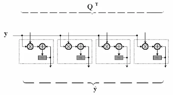
(62) 5.2 Matrix-Vector Multiplication Architecture Figure 5-3 details the array which computes the product QT y. One input of the array comes from the triangular systolic array of QR-decomposition. The other input is the current received vector y. The signal is input at the left of the array. This array is comprised of four multiply-accumulate cells. Each cell has the same structure shown in Figure 5-3. [Figure 5-3] Hardware realization of the matrix-vector multiplication array. 51.

(63) 5.3 Multistage K-Best Detection Architecture In this section, we describe the pipelined architecture for the implementation of the multistage K-Best algorithm. The architecture, shown in Figure 5-4, is composed of 2MT pipeline layers. Each layer represents one level of the tree and consists of q pipeline stages. The data path of the pipeline stage, shown in Figure 5-5, is almost the same. Each stage in these layers comprises three main entities: n The metric calculation unit computes the partial Euclidean distances of all. survivor paths. o The sorting network realizes the search-the-K-candidates-with-the-smallest-. partial-Euclidean-distance operation and forwards the smallest K values and the corresponding partial symbol vectors to the next pipeline stage. The partial Euclidean distance delivered by the metric calculation unit can be sorted in one clock cycle or in multiple clock cycles. In general, sorting in one clock cycle is not suited for the VLSI implementation because it yields prohibitive circuit complexity. Efficient sorting in the multistage K-Best algorithm is crucial to achieve a high throughput and low area. Therefore, the most popular method is that sorting is distributed over multiple cycles clocked at a higher clock rate. p The buffer is composed of two register banks. One stores the elements of. upper triangular matrix R and the elements of preprocessed vector information. yˆ . The other stores the hard bits and weight bits of the K survival vectors.. 52.

(64) [Figure 5-4] Pipelined architecture for multistage K-Best detector. [Figure 5-5] Hardware architecture of each layer. 53.

(65) 5.3.1 Sorting Network Within computer science many different sorting algorithms exist and are implemented. The classification of sorting algorithms into various families such as “ insertion ”, “ exchange ”, “ selection ”, etc., is not always clear. We will discuss three types of sorting algorithms in the following sub-sections. Exchanging is the dominant characteristic for these algorithms. The internal structures of the three different sorting networks are shown in Figure 5-6 ~ 5-8. The basic unit, a comparator used to perform a compare-exchange operation, takes in two data streams and either passes them unchanged or switches them. After comparing input U with input L, the objective is to ensure that max (U, L) is output on X and min (U, L) is output on Y.. [Figure 5-6] Bubble-sorting network for 16 inputs. 54.

(66) [Figure 5-7] Batcher’s bitonic-sorting network with I/O size 16. [Figure 5-8] Block diagram of M. Afghahi’s sorting network [37]. 55.

(67) 5.3.1.1 Bubble-Sort The general-purpose bubble-sorting network shown in Figure 5-6 for sorting N elements consists of N stages. In accordance with the data flow of the bubble-sorting network the individual disorganized elements which are called “keys” pass through a series of comparisons and exchanges. The keys that are sorted for our purposes will be in ascending or descending order. Although the interconnection between stages is small and the layout is regular, the architecture has an area of O (N2) and a delay of O (N) gates.. 5.3.1.2 Batcher’s Bitonic-Sort An ingenious way to program a sequence of comparisons, looking for potential exchanges, was discovered in 1964 by K.E. Batcher. Batcher’s method achieves the effects of 8-sorting, 4-sorting, 2-sorting, and 1-sorting, but the comparisons do not overlap. Since Batcher’s algorithm essentially merges pairs of sorted subsequences, it may be called the “ merge exchange sort ”. The standard N × N Batcher’s sorting network has O (log2 N) stages. Generally the Batcher’s sorting network is considered to have O (log2 N) time complexity and require O (Nlog2 N) two-input comparators for sorting N inputs. When the number N of data for sorting increases it is too difficult to obtain a corresponding Batcher’s sorting network because of more complex interconnection between stages. Batcher's bitonic sorting network shown in Figure 5-7 is merge-based sorting networks [36]. Each. column. accepts. data. from. the. previous. column,. performs. N/2. comparison-exchange steps in parallel, then passes the data onto the next column. With such parallel operations, sorting is completed in ( log 2 N)[( log 2 N) + 1] / 2 steps. 56.

(68) so that we require N( log 2 N)[( log 2 N) + 1] / 4 comparators. N is the number of data for sorting. Although this is about as fast as any general method known, it requires more complex interconnection between comparator modules.. 5.3.1.3. M. Afghahi’s Sort. The sorting network proposed by M. Afghahi shown in Figure 5-8 requires O (N) comparators [37]. When used in the sorting of a sequence in ascending order,. smaller key feeds back to the shift register of the cell and will compare with the next coming key and bigger key passes through the cell. It requires (N+1)β clock cycles to sort a sequence of N β-bits keys, where the clock period in these algorithms is the time required to compare and exchange only one bit of two keys, and β is the length of the keys. Therefore the processing time to sort a sequence is linearly proportional to the number of data and not proportional to the maximum number of cells in the system. A detailed discussion of the bit-serial sorter can be found in [37].. [Figure 5-9] Number of comparators in the different sorting network for various N. 57.