利用隱藏式馬可夫模型之棒球精彩事件短片偵測

(1)

利用隱藏式馬可夫模型之棒球精彩事件短片偵測

研究生：蔡維晉

指導教授：李素瑛

國立交通大學資訊科學與工程研究所

摘要

近年來棒球影像分析已有相當多的研究成果，但是對於精彩內容意涵事件偵測分類等影像處理技術的分析細膩度尚嫌不足。而這篇論文提出一個有效且有效率的棒球影片精彩內容意涵事件偵測分類系統，利用棒球影片中特定的場地規格及規律的場景轉換，使得此系統能夠辨識正在進行的精彩內容意涵事件。為了達到此一目標，本論文提出的系統概述如下:首先，我們可將一部棒球影片切割成精采短片，而每一個精彩短片開始於投手投球並結束於某些特定結束畫面，利用短片中每張畫面出現的物件特徵及順序，進而利用擷取出來的資訊用來發展以隱藏式馬可夫模型所建立的十二種精彩短片事件分類器。我們在此篇論文提出更精確的特徵擷取，使得棒球精采短片在分類上有著高準確性並且多樣性。此方法在運算上非常有效率，更重要的是，各種精采短片分類的實驗數據結果顯示相當良好的系統效能及準確性。檢索詞: 精采內容意涵事件偵測分類，特徵或物件擷取，隱藏式馬可夫模型。

(2)

Baseball Event Semantic Exploring System Using HMM

Abstract

Despite a lot of research efforts in baseball video processing in recent years, little work has been done in analyzing the detailed semantic baseball event detection. This thesis presents an effective and efficient baseball event classification system for broadcast baseball videos. Utilizing the strictly-defined specifications of the baseball field and the regularity of shot transition, the system recognizes highlight in video clips and identifies what semantic baseball event of the baseball clips is currently proceeding. The semantic exploring system is proposed to achieve the objective. First, a video is segmented into several highlights starting with a PC (Pitcher and Catcher) shot and ending up with a close-up or some specific shots. Before every baseball event classifier is designed, several novel schemes including some specific features such as soil percentage and objects extraction such as first base are applied. The extracted midlevel cues are used to develop baseball event classifiers based on an HMM (Hidden Markov model). Due to specific features detection the proposed method not only improves the accuracy of the highlight classifier but also supports variety types of the baseball events. The proposed approach is very efficient. More importantly, the simulation results show that the classification of twelve significant baseball highlights is very promising.

Index: highlight detection and semantic baseball event classification, features or objects extraction, Hidden Markov Model.

(3)

Acknowledgement

I greatly appreciate the kind guidance of my advisor, Porf. Suh-Yin Lee. Without her graceful suggestion and encourage, I cannot complete this thesis.

Besides, I want to give my thanks to my friends and all members in the Information System laboratory for suggestion, especially Mr. Hua-Tsung Chen.

Finally, I would like to express my appreciation to my parents for their supports. This thesis is dedicated to them.

(4)

List of Figures

Figure 2-1 Hierarchical structure of baseball game………...3

Figure 2-2 The conversion from RGB to HSI………4

Figure 2-3 Illustrates the block types……….5

Figure 2-4 Four baseball HMM defined in [5] (a) nice hit, (b) nice catch, (c) homerun, and (d) the play within the diamond (events occur in infield)…………...8

Figure 2-5 The seven pre-defined types of shots in [5]………9

Figure 2-6 The system overview of highlight detection and classification in [8]……9

Figure 2-7 Three shot transition types defined in [11]……….10

Figure 2-8 Twelve scoreboards defined in [11]………10

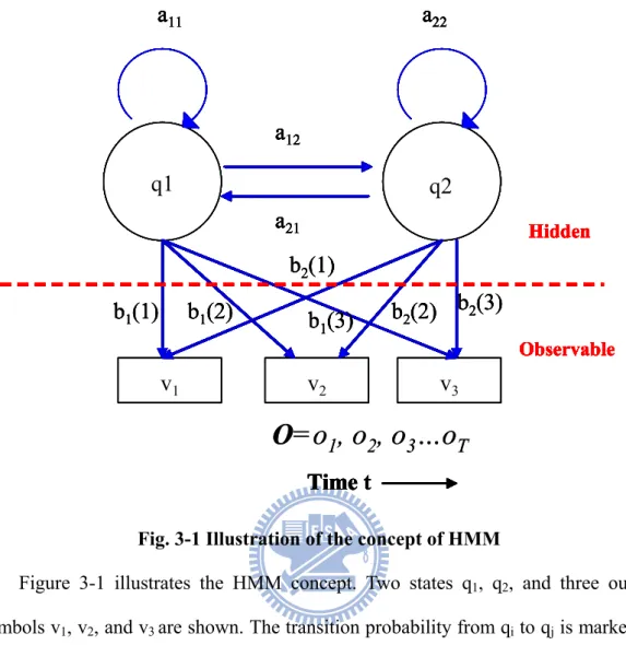
Figure 3-1 Illustration of the concept of HMM………13

Figure 3-2 Illustration of the forward algorithm of variable α_t

( )

i ……….15

Figure 3-3 The induction step of the forward algorithm………..17

Figure 3-4 The induction step of the backward algorithm………...18

Figure 3-5 Illustration of the sequence of operations required for the computation of the joint event that the system is in state Si at time t and Sj at time t+1...22

Figure 4-1 (a) Overview of the training step in proposed baseball event classification. (b) Overview of the classification step in proposed baseball event classification………....25

Figure 4-2 The color space of RGB and HSI of two baseball clips……….27

Figure 4-3 The process of finding dominant colors……….27

Figure 4-4 The field objects and features………28

Figure 4-5 Illustration of (a) back auditorium (b) left auditorium (c) right auditorium………..………28

Figure 4-6 Line pixel detection excluding large white area……….29

Figure 4-7 The result of retained high intensity pixel after line pixel detection algorithm:(a) original data (b) high intensity pixel before line pixel detection (c) high intensity data after line pixel detection……….30

(7)

Figure 4-9 Shows the objects of 1B, 2B, HB, LL, RL, and PM………..32

Figure 4-10 Deletion of illegal ellipse………...32

Figure 4-11 Sixteen typical frame types………...33

Figure 4-12 Illustrate the annotated string of ground out example after frame classification……….35

Figure 5-1 Comparison between (a) ground out and (b) double play………...43

Figure 5-2 Comparison between (a) right foul ball and (b) home run………..44

Figure 5-3 Ambiguity of (a) left foul ball (b) replay of left foul ball………44

Figure 5-4 Ambiguity of ground out and single………44

Figure 5-5 Ambiguity in second base………..45

Figure 5-6 3-state original Hidden Markov Model……….46

(8)

List of Tables

Table 4-1 Rule of frame type classification………..…………34

Table 4-2 Lists twelve highlights………..………36

Table 4-3 Lists HMM algorithm for baseball event………..……38

Table 5-1 Recognition of frame type manually cut………..….40

Table 5-2 Recognition of frame type automatic cut……….……40

Table 5-3 Recognition of highlight manually cut………..42

(9)

Chapter 1 Introduction

In recent years, the amount of multimedia information has grown rapidly. This trend leads to the development of efficient sports video analysis. Automatic sports video analysis has attracted considerable attention, because sport video appeals to large audiences. The possible applications of sports video analysis have been found almost in all sports, among which baseball is a quite popular one. However, a whole game is very long but the highlight is only a small portion of the game. In addition, highlight can be detected to provide a tactic for coaching. Based on these motivations, development of the highlight semantic exploring system for the baseball games is our focus.

Because the positions of cameras are fixed in a game and the ways of showing game progressing are similar in different TV channels. Each category of semantic baseball event usually has a similar shot transition. For example, a typical fly out can be composed of a pitch shot followed by an outfield left or center or right shot and then a play in grass shot. Based on this observation, many methods are applied on semantic baseball event detection such as HMM [5][6][7], temporal feature detection [8], BBN (Bayesian Belief Network) [11]. The existing highlight detection and classification systems suffer from atleast one of the flaws in the following: (1) only fewhighlights or mid-level semantics (lower than highlightsemantics) are detected, (2) the accuracy of classification is not high enough for practical usage, and (3) time complexity is rather high. To solve the problems of existing highlight detection or classification systems, high accuracy and more specific highlight especially hitting highlight (ball has been hit) detection and classification, is our foremost target.

This thesis presents an HMM-based mechanism to detect and classify baseball events. To improve the accuracy of baseball event classification and specific baseball

(10)

event classification, more features and objects (lower than highlightsemantics) must be detected. Twelve semantic baseball event types in baseball games are defined and detected in the proposed system: (1) single (2) double (3) pop up (4) fly out (5) ground out (6) two base hit (7) right foul ball (8) left foul ball (9) foul out (10) double play (11) home run (12) home base out. Some mid-level semantics are introduced in the following section and these mid-level semantics are used to detect and classify baseball events. In the proposed framework, highlight detection and baseball event classification in broadcast baseball videos will be more powerful and practical, since comprehensive and detailed information about the game can be presented to users.

The rest of the thesis is organized as the follows. The background and related works are introduced in chapter 2. In chapter 3, we introduce the HMM concept used in our system. Chapter 4 introduces our proposed system including feature extraction, frame classification, baseball event classification. Chapter 5 shows the experimental results and discussion. Finally, conclusion and future work are made in chapter 6.

(11)

Chapter 2 Background and Related Works

In chapter 2, the baseball highlight detection in recent years will be introduced. First of all, we will describe the hierarchical structure of a baseball game in section 2-1. In section 2-2, image processing of color space conversion from RGB to HSI is introduced to make some tasks easily such as less influence on luminosity. In the following sections, some related works in PC (Pitcher and Catcher) shot detection, and highlight detection for baseball videos are depicted.

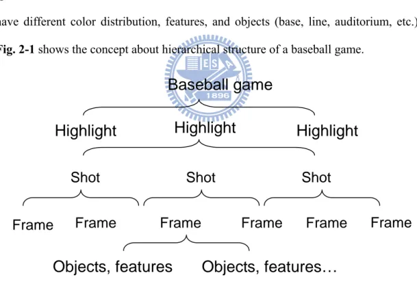
2.1 Hierarchical Structure of Baseball Game

A baseball game is composed of some highlights. Highlight is a sequence of specific shot transition. A shot consists of several similar frames. Different frames have different color distribution, features, and objects (base, line, auditorium, etc.).

Fig. 2-1 shows the concept about hierarchical structure of a baseball game.

Fig. 2-1 Hierarchical structure of baseball game.

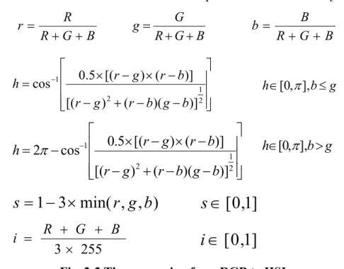
2.2 Color Conversion from RGB to HSI

In image processing, color is an important feature. The influence on luminosity of HSI is less than that of RGB. To make feature extraction or objection detection easily, we can use the following formula as described in Fig. 2-2 to convert from

Frame

Baseball game

Highlight

Shot Shot

Shot

Frame

(12)

RGB to HSI. Similar skill can be found in other sports such as basketball [19]. B G R G g + + = B G R R r + + = B G R B b + + = ⎥ ⎥ ⎥ ⎦ ⎤ ⎢ ⎢ ⎢ ⎣ ⎡ − − + − − × − × = − 2 1 2 1 )] )( ( ) [( )] ( ) [( 5 . 0 cos b g b r g r b r g r h

⎥

⎦

⎤

⎢

⎣

⎡

−

+

−

×

−

×

−

=

− 2 1 2 1

)]

)(

(

)

[(

)]

(

)

[(

5 .

0 cos

2 b

g

b

r

g

r

b

r

g

r

h

π

g b h∈[0,π], ≤ g b h∈[0,

π

], >

)

,

min(

3

1 r

g

b

s

=

−

×

s

∈

[

0 ,

1 ]

255

3 ×

+

=

R

G

B

i

_i

∈

_[

₀

_,

₁

_]

Fig. 2-2 The conversion from RGB to HSI. 2.3 Pitcher and Catcher Shot (PC shot) Detection

Every baseball highlight starts with PC shot and ends up with some specific shots or a close-up shot, so the PC shot detection plays an important role in baseball highlight detection. The proposed method in [1] based on feature mining can find the effective feature types, the location of the features and threshold values during the learning process.

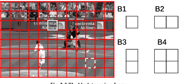
In general, the composition of the PC shot is auditorium, player, soil and grass. However, it has some unstable elements. The location and uniform of players would be changing. Features without influences on these changes (i.e. location of player) are that the PC shot is composed of ground, wall, and audience. To find the features, an image is divided into 12 × 8 blocks as shown in Fig. 2-3.

(13)

B1

B2

B3

B4

B1

B2

B1

B2

B1

B2

B3

B4

B1

B2

B1

B2

B1

B2

B3

B4

B1

B2

B3

B4

B1

B2

B1

B2

Fig. 2-3 The block types in a frame.

Then we use mean, variance, and log variance on luminosity data to discover the effective blocks (effective block will be elaborated later) for PC shot discrimination in training data. In experiment, we use four block size as a unit, B1, B2, B3, and B4 to calculate the mean, variance, and log variance. Some trends are observed as follows.

(1) The mean of the luminosity in the ground block, as shown by white dotted line in Fig. 2-3, is stable even if a camera shift takes place.

(2) The variance of the luminosity in the ground block is small because the ground is

flat in the block.

(3) In a wall block as shown by white solid line, the variance becomes large due to the

high texture, but the log variance can be assumed to be stable in the block.

We assume that fusion of these three features is effective in PC shot discrimination. Next, desirable features should be stable at the same location in the training data set, so the block with small variance of the feature called effective block in the training data is thought of as the best location of those blocks.

The X-axis of an image is divided into 12 blocks and the Y-axis is divided into 8 blocks of the image as shown in Fig. 2-3. Four block types B1, B2, B3 and B4 are used to search for the effective blocks for PC shot discrimination. The mean Mf,t,z, the variance Vf,t,z, and the log variance LVf,t,z computed within the block type t and the

(14)

location i t i

B , is defined by Eq.(l), Eq.(2), and Eq.(3). Here, t (t = 1~4) and i (i = 1~96, 1~48, or 1~24 depends on different block type) indicate the block type and block position counted from top-left corner in a frame f respectively. Let Gray(x, y) denote the luminosity at location (x, y) of the image and |B| denote the number of pixels in a block.

(

)

∑

∈

=

t i B y x, i t, f,

Gray

x

y

B

M

_t i

,

1

(1)

(

)

(

)

2

,

1 ∑

∈

−

=

t i B y x, f,t,i i t, f,

_B

Gray

x

y

M

V

_t i (2)

(

)

(

)

2

,

log

1 _∑

∈

−

=

t i B y x, f,t,i i t, f,

Gray

x

y

M

B

LV

_t i (3)

Let N be the number of PC shots in training data. The variance of the mean in the block

B

_it among the training data is defined in Eq. (4).

2 1 1

1

1 ∑

∑

= =

⎟⎟

⎠

⎞

⎜⎜

⎝

⎛

−

=

N f N f

M

N

M

N

V

_M,_t,_i _f,_t,_i _f,_t,_i ₍₄₎

When all V_M _,_t_,_i for all t and i are placed in ascending order, the variance at rank n

is defined as n M i M t M V _, _, . The block tM M i

B at the rank 1 with variance

V

M1,tM,iM is regarded as the optimal block in mean luminosity. Max and min value (threshold) of block luminance mean

M i M t f M _, _, at frame f in block tM M i

B is defined by Eq. (5) and (6) respectively.

(

f,t_M i,_M

)

f max M i, M, t

M

=

max

₍₅₎

(

f,t_M ,i_M

)

f min M i , M, t

M

=

min

₍₆₎

(15)

calculated respectively. The optimal block in variance and log variance are found of rank 1V_V1_,_t_,_i,V_LV1 _,_t_,_i . Max and min value (threshold) of block luminance variance

and log variance are min,

max , min , max , , , , , M

,

M M

,

M M

,

M M M i t i t i t i t

V

LV

V

_{. Last, if a test image f’}

meets the conditions in Eq. (7), the image f’ is viewed as a PC shot.

max , , , , ,' min , , max , , , , ,' min , , max , , , , ,' min , , M i M t M i M t f M i M t M i M t M i M t f M i M t M i M t M i M t f M i M t

LV

V

M

≤

(7)

This method [1] showed 95.5% accuracy at F-measure score within 1/30 of real time.

2.4 Highlight Detection and Classification

Highlight detection and classification is a popular issue as a result of the following reasons: (1) Provide coach with a guidance of tactic, (2) Make a highlight movie, (3) Index each highlight used for baseball event retrieval, and (4) More accurate in baseball event classification from baseball game. In the past few years, significant research [5, 6, 7, 8, 9, 10, 11] has been devoted to the content analysis of baseball game. [5][6][7] use the statistical model of HMM to detect and classify the highlights. For example, Chang et al. [5] assumes that most highlights in baseball games consist of certain shot types and these shots have similar transition in time. Each highlight is described by an HMM as shown in Fig. 2-4 and each hidden state is represented by its predefined shot types as shown in Fig. 2-5. Some features are used as observations to train the HMM model for highlight recognition.[5][6] use some features and shots as observations and states in HMM for highlight classification. Low accuracy and few highlight types are the main disadvantages because the information is too little to detect various highlights and to get high accuracy. [8] records some objects or features such as field type, speech, and camera motion start

(16)

time and end time to find the frequent temporal patterns as shown in Fig. 2-6 for highlight detection and classification. The accuracy in [8] is better than that in [5][6], but they use speech, caption and shot as features so that the cost of time complexity is high. [9][11] combine some shots such as pitch and catch, infield, outfield, and non-field shot with scoreboard as shown in Fig. 2-7 and Fig. 2-8 as medium-level cues, and then use Bayesian Belief Network (BBN) structure for highlight classification. [10] uses some condition rules for highlight classification. [9][11] use scoreboard as additional information so that the accuracy is very high, but the rough shot classification lead to the low variety of hitting highlight.

In this thesis, we will emphasize the variety of baseball events and high accuracy via more features and objects exploration. Statistical model HMM is used for highlight classification and HMM concept will be elaborated in chapter 3.

Fig. 2-4 Four baseball HMMs defined in [5] (a) nice hit, (b) nice catch, (c) homerun, and (d) the play within the diamond (events occur in infield)

(17)

Pitch view Catch overview Catch close-up Running overview

Running close-up Audience view Touch base close-up

Pitch view Catch overview Catch close-up Running overview

Running close-up Audience view Touch base close-up

Fig. 2-5 The seven pre-defined types of shots in [5].

Pitch scene

Pan up

Field scene

Cheer

Ex. home run

Visual content stream

Camera motion stream

Audio content stream

Pitch scene

Pan up

Field scene

Cheer

Ex. home run

Pitch scene

Pan up

Field scene

Cheer

Ex. home run

Pitch scene

Pan up

Field scene

Cheer

Pitch scene

Pan up

Field scene

Cheer

Ex. home run

Visual content stream

Camera motion stream

Audio content stream

(18)

Fig. 2-7 Three shot transition types defined in [11].

(19)

Chapter 3 Hidden Markov Model

Real-world processes generally produce observable outputs which can be characterized as signals. Finding the regular rule in those signals is a popular issue in real world (e.g., the sequence of instruction in computer, the sequence of speech recognition, etc). It is required to build signal models to analyze the real-world signal, and then these signal models can be realized into applications in practical systems such as prediction system, recognition system, identification system, etc.

Generally, signal models can be classified into deterministic models, and statistical models. In practical systems, deterministic models are used to exploit the specific rules of the signal such as traffic light. The current state can be determined easily by the previous state. The other case of signal model is statistical model which is modeling a wide range of time series data like Poisson process, Markov model, Hidden Markov Model and so on. In this case, the next state cannot be determined by current state, but a model is still created to estimate signal properties even if the model would miss some messages.

Among statistical models, Hidden Markov model is a powerful statistical model for modeling the generative sequence in many fields such as biology, mathematics, speech recognition, signal processing. Differing from Markov model, the state is not observable. Because features and shot transitions can be viewed as observable outputs and states, a highlight can be described by a signal model such as HMM. When an observable signal is given, the likelihood was computed by each signal model and the best match is the proposed highlight.

3.1 Element of an HMM

A Hidden Markov model has several states, each of which has a transition probability from current state to next state and the next state is only dependent on the

(20)

current state. Each state has several output symbols but yields a symbol at one time. Each symbol has an output probability and the output symbol at time t is dependent only on the current state. Some notations are defined as follows:

T = length of the observation sequence. N = the number of states in the model. M = the number of observation symbols. The set of N states: Q=

{

q₁,q₂,...,q_N

}

The set of M output symbols (observations): V =

{

v₁,v₂,...,v_M

}

States : Which state belongs to at time t, _t

s

_t

∈

Q

(unobservable). For example, i

t q

s = is a representation of staying in state qi at time t.

The state transition probability: A=

{

a_ij |a_ij =P_r

(

s_t₊₁ =q_j |s_t =q_i

)

|1≤i,j≤N

}

The output symbol probability: B=

{

b_j

( )

k =P_r

(

v_k |s_t =q_j

)

|1≤ j≤N,1≤k ≤M

}

The initial probability: π=

{

π_i |π_i = P_r

(

s₁ =q_i

)

|1≤i≤N

}

Parameter set of HMM modelλ=

{

A,B,π

}

Observed symbol sequence O=o₁,o₂,...,o_T(length=T)

(21)

q1

q2

a

₁₁

a

₂₂

a

₁₂

a

₂₁

v

₁

v

₂

v

₃ Hidden Observable

Time t

q1

q2

a

₁₁

a

₂₂

a

₁₂

a

₂₁

v

₁

v

₂

v

₃

b

₁

(1)

Hidden Observable

Time t

b

₁

(2)

_b

1

(3)

b

₂

(1)

b

₂

(2) b

2

(3)

q1

q2

a

₁₁

a

₂₂

a

₁₂

a

₂₁

v

₁

v

₂

v

Time t

q1

q2

a

₁₁

a

₂₂

a

₁₂

a

₂₁

v

₁

v

₂

v

₃

b

₁

(1)

Time t

b

₁

(2)

_b

1

(3)

b

₂

(1)

b

₂

(2) b

2

(3)

O=o

₁

, o

₂

, o

₃

…o

_T

q1

q2

a

₁₁

a

₂₂

a

₁₂

a

₂₁

v

₁

v

₂

v

Time t

q1

q2

a

₁₁

a

₂₂

a

₁₂

a

₂₁

v

₁

v

₂

v

₃

b

₁

(1)

Time t

b

₁

(2)

_b

1

(3)

b

₂

(1)

b

₂

(2) b

2

(3)

q1

q2

a

₁₁

a

₂₂

a

₁₂

a

₂₁

v

₁

v

₂

v

Time t

q1

q2

a

₁₁

a

₂₂

a

₁₂

a

₂₁

v

₁

v

₂

v

₃

b

₁

(1)

Time t

b

₁

(2)

_b

1

(3)

b

₂

(1)

b

₂

(2) b

2

(3)

O=o

₁

, o

₂

, o

₃

…o

_T

Fig. 3-1 Illustration of the concept of HMM

Figure 3-1 illustrates the HMM concept. Two states q1, q2, and three output symbols v1, v2, and v3 are shown. The transition probability from qi to qj is marked as directed line aij. Each state could produce an observation at one time and each observation is assigned an output probability.

The first time to enter which state of HMM is stochastically determined by an initial state matrix π. The transition probability of each state to other state is determined by a transition probability matrix A. If there are N states, the matrix A is an N×N matrix. Note that the HMM can transit from a state to itself. Each state of the HMM stochastically outputs a symbol at a time determined by a matrix B. If there are M output symbols, the matrix B is an N×M matrix. Time from 1 to T, the HMM will output symbolO=o₁,o₂,...,o_T, but the state transition sequence is non-observable.

A recognition process can be proceeded by given the tuple λ = {A, B, π} of an HMM model, and the matrix A, B, and π can be learned in HMM training stage.

(22)

In recognition process, the HMM with the highest probability will be chosen as a recognized result. Recognizing time-sequential symbols is equivalent to determining which HMM produce the output symbols. Section 3.2 and section 3.3 will describe the recognition process and the learning process for an HMM signal model.

3.2 Recognition Process in HMM

One HMM is created for each category for recognizing time-sequential observed symbols. In recognition phase, we will compute the probability Pr(O| λ) for each category and the best matches will be chosen as the proposed answer from all HMMs of a given observationO=o₁,o₂,...,o_T. That is,

Give an observation, O=o₁,o₂,...,o_T

Each HMM has a tuple

(

_Ai_,_Bi_,_πi

)

i =

λ i=1,2,...,C (if there are C categories) Proposed answer = arg max (Pr (λi| O))

The probability of the observation sequence of a given model is equivalent to evaluating how well a model predicts a given observation sequence. So now the current problem is how to compute the probability Pr (O| λ) of an observation sequence O and a given HMM λ.

The most straightforward way to compute the probability of the observations O

(O = o1, o2 … oT) for a specific state sequence Q (Q=q1q2q3….qT) is:

(

| ,

)

( | , ) ₁( ₁) ₂( ₂) ... ( ) 1 t t q q qT T T t P o q b o b o b o Q P =∏ = × × × = λ λ O (8)

and the probability of the state sequence is:

(

Q

)

q aqq aq q aq q aqT qT

P |λ =π ₁ ₁ ₂ ₂ ₃ ₃ ₄... ₋₁ (9)

So we can calculate the probability of the observations given the model as:

( )

|

(

|

,

) ( )

|

(

)

₁₂ ₂

(

₂

)

₂ ₃

...

₁

(

)

... 2 1 1 1 1 qq q q q qT qT qT T path all qT q q q q Q

o

b

a

o

b

a

o

b

Q

P

Q

P

₋ ∈

∑

=

λ

π

λ

O

₍₁₀₎

(23)

involved in the calculation is in the order of NT. This is very time consuming even if the length of the sequence T is moderate.

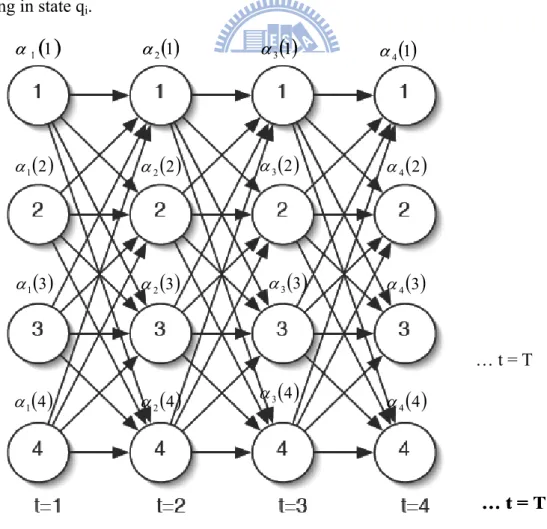
It is observed that many redundant calculations would be made by directly evaluating Eq. (10), and therefore caching the intermediate calculations can result in time complexity reduction. The cache is implemented as a trellis of states at each time stage, calculating the cached value (called α) for each state as a sum over all states at the previous time step. α is the probability of the partial observation sequence

o1 o2 … ot in state qi at time t. The concept is shown in Fig. 3-2 and the forward probability variable is defined in Eq. (11).

( )

(

λ

)

α_t i =P_r o₁,o₂,...,o_t,s_t =q_i | (11)

Eq. (11) describes the probability of the partial observation sequence from 1 to t, ending in state qi.

( )

2 1 α … t = T

( )

1 1 α

( )

2 1 α

( )

3 1 α

( )

4 1 α

( )

1 2 α

( )

2 2 α

( )

3 2 α

( )

4 2 α

( )

1 3 α

( )

2 3 α

( )

3 3 α

( )

4 3 α

( )

1 4 α

( )

2 4 α

( )

3 4 α

( )

4 4 α

( )

2 1 α … t = T … t = T

( )

1 1 α

( )

2 1 α

( )

3 1 α

( )

4 1 α

( )

1 2 α

( )

2 2 α

( )

3 2 α

( )

4 2 α

( )

1 3 α

( )

2 3 α

( )

3 3 α

( )

4 3 α

( )

1 4 α

( )

2 4 α

( )

3 4 α

( )

4 4 α

Fig. 3-2 Illustration of the forward algorithm of variable α_t

( )

i … t = T

(24)

In Fig. 3-2, in each time step, the partial probability αt of each state (trellis) is filled and the sum of the final column of the trellis will equal the probability of the observation sequence. The algorithm for this process is called the forward algorithm and is as follows: 1. Initialization

( )

i = _ib_i

( )

o₁ , 1≤i≤N 1 π α (12) 2. Induction

( )

j N

( )

i a b_j

( )

o_t t T j N i t ij t ⎥ ≤ < ≤ ≤ ⎦ ⎤ ⎢ ⎣ ⎡ = ₊ = +

∑

1 1 , 1 1 1 α α (13) 3. Termination

(

)

_∑

( )

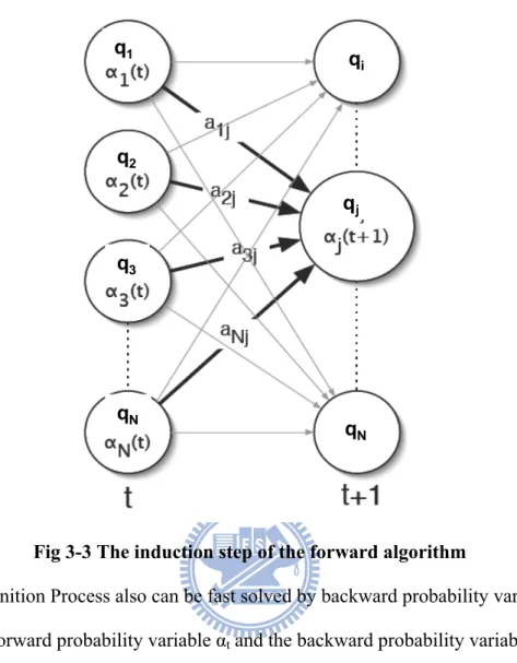
= = N i T i P 1 |λ α O (14)

The induction step is the key to the forward algorithm as shown in Fig. 3-3. In Eq(13), index j and i represent the current state index and previous state index respectively. For each state qj, αt(j) stores the probability of arriving in that state having observed the observation sequence up to time T. In termination step, adding up each forward partial variable σT is the probability of the observation produced from the HMM model. It is obvious that by caching α values the forward algorithm reduces the time complexity of calculations involved from 2TNT to N2T.

(25)

q₁ q₂ q₃ q_N q_N q_j q_i q₁ q₂ q₃ q_N q_N q_j q_i

Fig 3-3 The induction step of the forward algorithm

Recognition Process also can be fast solved by backward probability variable similar to forward probability variable αt and the backward probability variable is defined in Eq. (15).

( )

(

λ

)

β_t i =P o_t₊₁o_t₊₂...o_T |s_t =q_i, (15)

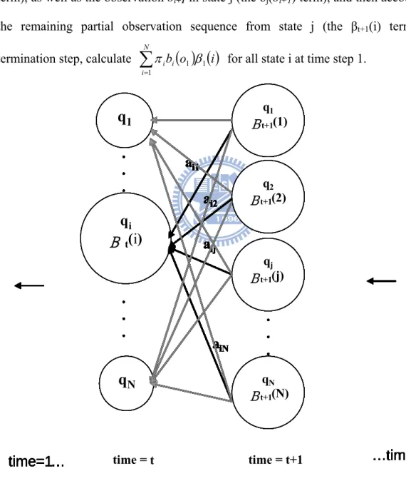
Eq. (15) describes the probability of the partial observation sequence from time t + 1 to T, starting in state qi. The algorithm for this process is called the backward algorithm and is as follows:

1. Initialization

( )

i =1 T β 1≤i≤ N (16) 2. Induction

( )

j N a

( ) ( )

j b_j o_t t T i N j t ij t = + ≤ < ≤ ≤ = +

∑

₁ , 1 , 1 1 1 β β (17)

(26)

3. Termination

(

)

_∑

( ) ( )

= = N i i ib o i P 1 1 1 |λ π β O (18)

The initialization step defines βT(i) to be 1 for all state i at time T. The induction step computes the partial probability of all states at time t from time t+1 as shown in Fig. 3-4. All possible states qi at time t+1 account for the transition from qi to qj (the aij term), as well as the observation ot+1 in state j (the bj(ot+1) term), and then account for

the remaining partial observation sequence from state j (the βt+1(i) term). In termination step, calculate

∑

( ) ( )

= N i i i i o b 1 1 1 β

π for all state i at time step 1.

S

₁

S

_N

S

_i

Β

t

(i)

S1 Βt+1(1) S2 Βt+1(2) Sj Βt+1(j) SN Βt+1(N)

.

a

_i1

a

_i2

a

_ij

a

_iN

.

time = t+1

time =

…time=T

time=1…

S

₁

S

_N

S

_i

Β

t

(i)

.

a

_i1

a

_i2

a

_ij

a

_iN

.

time = t+1 time =

S

₁

S

_N

S

_i

B

t

(i)

.

a

_i1

a

_i2

a

_ij

a

_iN

.

time = t+1 time = t

time=1…

S

₁

S

_N

S

_i

Β

t

(i)

.

a

_i1

a

_i2

a

_ij

a

_iN

.

time = t+1

time =

…time=T

time=1…

S

₁

S

_N

S

_i

Β

t

(i)

.

a

_i1

a

_i2

a

_ij

a

_iN

.

time = t+1 time =

q

₁

q

_N

q

_i

B

t

(i)

q1 Βt+1(1) q2 Βt+1(2) qj Βt+1(j) qN Βt+1(N)

.

a

_i1

a

_i2

a

_ij

a

_iN

.

time = t+1 time = t

time=1…

S

₁

S

_N

S

_i

Β

t

(i)

.

a

_i1

a

_i2

a

_ij

a

_iN

.

time = t+1

time =

…time=T

time=1…

S

₁

S

_N

S

_i

Β

t

(i)

.

a

_i1

a

_i2

a

_ij

a

_iN

.

time = t+1 time =

S

₁

S

_N

S

_i

B

t

(i)

.

a

_i1

a

_i2

a

_ij

a

_iN

.

time = t+1 time = t

time=1…

S

₁

S

_N

S

_i

Β

t

(i)

.

a

_i1

a

_i2

a

_ij

a

_iN

.

time = t+1

time =

…time=T

time=1…

S

₁

S

_N

S

_i

Β

t

(i)

.

a

_i1

a

_i2

a

_ij

a

_iN

.

time = t+1 time =

q

₁

q

_N

q

_i

B

t

(i)

q1 Βt+1(1) q2 Βt+1(2) qj Βt+1(j) qN Βt+1(N)

.

a

_i1

a

_i2

a

_ij

a

_iN

.

time = t+1 time = t

time=1…

Fig. 3-4 The induction step of the backward algorithm.

We can solve the recognition process problem in time complexity N2T by using forward algorithm or backward algorithm. Each HMM will output a probability and

(27)

the best match will be chosen as a recognized result.

3.3 HMM Training (learning)

The most difficult problem of HMMs is to determine a method to adjust the model parameters λ = (A, B, π) to maximize the probability of the observation

sequence given the model. Given any finite observation sequence as training data, there is no optimal method to estimate the model parameter. However, we can use an iterative procedure such as Segmental K-means algorithm [13] or Baum-Welch algorithm [18] to maximizeP O

(

, I |λ

)

(I is the optimal state sequence) orP

(

O|λ

)

. In Segmental K-means algorithm the parameters of the model λ = (A, B, π) are adjusted

to maximize P O

(

, I|λ

)

where I here is the optimal state sequence as given by the Viterbi algorithm [14]. In Baum-Welch re-estimation, here parameter of the model λ = (A, B, π) are adjusted so as to increase P

(

O|λ

)

until a maximum value is reached. As seen before, calculating P

(

O|λ

)

involves summing upP O

(

,Q|λ

)

over all possible state sequenceQ

(

Q=q₁q₂q₃...q_T

)

. Hence Baum-Welch algorithm dose not focus on a particular state sequence. The two methods will be described as follows respectively.

K-means algorithm takes us from _{λ to}k _λk+1_{(iteration k to k+1) such that}

(

) (

* 1

)

1 *_| _, _| , ≤ ₊ k+ k k k λ P I λ I PO O where, * k

I is the optimum state sequence for T

o o o₁, ₂..., =

O and_λk_{, found according to the Viterbi algorithm. The criterion of} optimization is called the maximum state optimized likelihood criterion. This

function _P

(

,_I*|λ

)

max _P

(

,_I |λ

)

I O

O = is called the state optimized likelihood function. Training the model in K-means Algorithm, a number of (training)

observation sequences are required. Let there be w sequences available. Each sequence consists of T observation and each observation symbol

( )

o is assumed to _i be a vector of dimension D

(

D≥1

)

. K-means Algorithm then consists of the following

(28)

steps:

1. Randomly choose N observation symbols (map vector of dimension D to symbol by rule table) and assign each of the wT observation symbols to one of these N symbols from which its Euclidean distance is minimal. Hence we have formed N clusters, each of which is called a state (1 to N). We can divide those training data into N groups and pick one observation vector from each group. Of course this method is just to make the initial choice of states as widely distributed as possible. 2. Calculate the initial probabilities and the transition probabilities. i, and j represent

the current state index and next state index and t represents time from 1 to T-1:

sequence of number Total o of s occurrence of Number ₁ ⎭ ⎬ ⎫ ⎩ ⎨ ⎧ ∈ = i state i π , 1≤i≤ N (19) ⎭ ⎬ ⎫ ⎩ ⎨ ⎧ ∈ ⎭ ⎬ ⎫ ⎩ ⎨ ⎧ _∈ _∈ = + i state j state o i state a t ij t 1 t o of s occurrence number Total , o of s occurrence of Number N i≤ ≤ 1 ,1≤j≤N (20) 3. Calculate the mean vector and the covariance matrix for each state: for 1≤i≤N

i, and j represents current and next state index, t represents time from 1 to T:

∑

∈

=

i state o t i t

o

N

1 μ

₍₂₁₎

(

) (

)

∑

∈

−

=

i state o i t T i t i t

o

N

V

1 μ

μ

(22)

4. Calculate the symbol probability distributions for each training vector for each state as (assume Gaussian distribution – change the formulas below for the particular probability distribution that suits problem). For 1≤i≤N, i represents state index and t represents time from 1 to T

(29)

( )

(

) (

)

⎥⎦ ⎤ ⎢⎣ ⎡₋ ₋ ₋ = _t _i _i− _t _i T i D t i o V o V o b μ μ π 1 2 / 1 2 / 2 1 exp 2 1 (23)

5. Find the optimal state sequence _{I (as given by Viterbi algorithm) for each}* training sequence using λ =

(

A ,,B π

)

computed in step2 to 4 above.

π B,

A, and are the new state transition, output symbol, and initial state probability respectively from re-estimation. Each observation symbol is reassigned a state if its original assignment is different from the corresponding estimated optimum state.

6. If any observation symbol is reassigned a new state in step5, use the new assignment and repeat step2 through step6; otherwise, stop.

It can be shown in [15] that Segmental K-means algorithm converges to the state-optimized likelihood function for a wide range of observation density functions including Gaussian density function.

The second method is called Baum-Welch algorithm, assuming that an initial model can be improved upon by using the Eq. (30)-(32). An initial HMM can be constructed in any way such as random generation, but we may use the first five steps of the Segmental K-means algorithm described above to give us a reasonable initial estimate of the HMM and use Baum-Welch algorithm to re-estimate. Before we get down to the actual Eq. (30)-(32) of Baum-Welch algorithm, some concepts and notations should be introduced that shall be required in the final Eq. (30)-(32).

The forward-backward variable γt is defined in Eq. (24).

( ) (

)

( ) ( )

₍

₎

( ) ( )

∑

= = = = = _N i t t t t t t T i t t i i i i P i i o o o q s P i 1 2 1 | , ,... , | β α β α λ β α λ γ O (24)

Eq. (24) describes the probability of being at state qi in time t. To describe the procedure of re-estimation (iterative update and improvement) of HMM parameter,

(30)

the variable ε_t

( )

i,j was defined in Eq. (25) and Eq. (25) describes the probability of being at state qi in time t and at state qj in time t+1.

( )

(

λ

)

ε

_t

i

,

j

=

P

s

_t

=

q

_i

,

s

_t₊₁

=

q

_j

|

O

,

(25)

The sequence of events leading to the conditions required by Eq. (25) is illustrated in

Fig. 3-5. It should be clear, from the definitions of the forward variable αt(i) and backward variable βt(i), that we can re-write Eq. (25) in the following form

( )

₍

( ) ( )

₎

( )

( ) ( )

( )

( ) ( )

∑∑

= = + + + + + +

=

_N i N j t t j ij t t t j ij t t t j ij t

j

o

b

a

i

j

o

b

a

i

P

j

o

b

a

i

j

i

t 1 1 1 1 1 1 1 1

|

,

β

α

β

α

λ

β

α

ε

O

(26)

where the numerator term is justP

(

s_t=q_i,s_t₊₁ =q_j |O,λ

)

and the division byP

(

O|λ

)

gives the desired probability measure.

. . . . . . . . .

t

t+1

t-1

t+2

q

_i

q

_j

a

_ij

b

_j

(o

_t+1

)

α

_t

(i)

β

_t+1

(j)

. . . . . . . . . . . . . . . . . . . . . . . . . . .

t

t+1

t-1

t+2

q

_i

q

_j

a

_ij

b

_j

(o

_t+1

)

α

_t

(i)

β

_t+1

(j)

Fig. 3-5 Illustration of the sequence of operations required for the computation of the joint event that the system is in state qi at time t and qj at time t+1

If we sum up forward-backward variable γt(i) from t=1 to T at each state i, we get a quantity which can be viewed as the expected number of times that state qi is visited, or if we sum up only to T-1 then we shall get the expected number of transitions out of state qi (as no transition is made at t = T). Similarly if εt

( )

i,j be summed up from t=1 to T-1, we shall get the expected number of transitions from state qi to state qj. Hence

(31)

( )

expectednumber of timesstateq_iis visited. 1 =

∑

= T t t i γ (27)

( )

=

∑

− = 1 1 T t t i

γ expectednumber of transition fromq_i (28)

( )

=

∑

− = 1 1 , T t t j i

ε expectednumber of transitionsfromq_i toq_j. (29)

Using above formulas we can give a method for re-estimation of the parameter of an HMM. A set of reasonable re-estimation formulas for A, B, and πare

) , ( matrix y probabilit state initial new is and matrix on distributi symbol output new is matrix y probabilit transition state new is π B , A (i). 1) at time(t q state in being times of number expected _i γ₁ π_i = = = (30)

(index i represents the state i)

( )

∑

− = − = = = 1 1 1 1 ij , exp exp a T t t T t t i j i i j i q state from s transition of number ected q state to q state from s transition of number ected γ ε (31)

( )

∑

= = = = = = T t t T t t i i M k 1 k t 1 j k j j v s.t.o q state in times of number expected ) ~ 1 ( v symbol observing and q state in times of number expected k b γ γ ₍₃₂₎

If the initial model λ = (A, B, π) is defined, we use Eq. (27)-(29) to compute the

right hand sides of Eq. (30)-(32) for λ=

(

A,B,π

)

. Baum and his colleagues prove that either (1) the initial model λ defined a critical point of the likelihood function, in which caseλ =λ; or (2) model λ is more likely than model λ in the sense that P

( )

O|λ >P

(

O|λ

)

, i.e. a new model λ has been found from which the

(32)

observation sequence is more likely to have been produced. We can improve the probability of O which is being observed from the model if we repeat the above

procedure and use λ to replace the λ several times until some limiting point is reached. The final result of re-estimation is called a maximum likelihood estimate of the HMM.

(33)

Chapter 4 Proposed scheme for Event classification

4.1 Overview of Proposed Scheme

Overview of the proposed semantic baseball event classification is depicted in

Fig. 4-1(a), and Fig. 4-1(b). The process can roughly be divided into two steps:

training step and classification step. In training step, each type as listed in Table 4-2

of indexed baseball event was input as training data for each highlight classifier. In classification step, when each observation symbol sequence of unknown clip was input, each highlight classifier will evaluate how well a model predicts a given observation sequence.

HMM training

1.Training Step

Several indexed baseball clips in each type

Color conversion

Object detection

Until the last key frame

Frame classification

Rule

table

HMM 1 HMM 2 HMM 3 . . . HMM 12 HMM training 1.Training Step

Several indexed baseball clips in each type

Frame classification

Rule

table

HMM 1 HMM 2 HMM 3 . . . HMM 12 HMM 1 HMM 2 HMM 3 . . . HMM 12

Fig. 4-1(a) Overview of the training step in proposed baseball event classification

2.Event classification step

Unknown clip Frame classification

Rule

table

HMM 1 HMM 2 HMM 3 . . . HMM 12 Event type is determined 2.Event classification step

Unknown clip Frame classification

Rule

table

HMM 1 HMM 2 HMM 3 . . . HMM 12 HMM 1 HMM 2 HMM 3 . . . HMM 12 Event type is determined

Fig. 4-1(b) Overview of the classification step in proposed baseball event classification

Each highlight clip as input starts with a PC shot and ends up with a close-up shot or a specific shot depending on different baseball event type. There are

(34)

considerably many uninteresting segments in a baseball game video (e.g., commercials). Hence, some pre-processing schemes such as PC shot [1] and close-up shot detection are needed to trim out these segments.

As the section 2-1 described, a highlight is composed of some shots, each of which consists of several objects and features. To classify highlight, some tasks such as object and feature detection should be solved in the preliminary. In order to make the object detection easily, techniques of image processing are applied. An observation sequence is generated after feature extraction and object detection. Symbols mapped from feature vector by rule table are used as observations, and the number of states represented as shots are empirically determined. Then, we use Segmental K-means algorithm to create an initial HMM parameter λ and Baum-Welch algorithm to re-estimate highlight HMM parameterλ. In classification step, an observations sequence is generated after feature extraction and object detection, too. Each event of baseball highlight HMM will output a probability and the best match will be chosen as the proposed answer. Extracted features and detected objects are used for frame classification by a rule table as listed in Table 4-1 modified

from [4] for the purpose of realizing the transition of shots. Details of the proposed approaches are described in the following sections. Section 4-2 introduces the color conversion. Section 4-3 describes object and feature detection. Section 4-4 describes frame classification. Section 4-5 and section 4-6 describe HMM learning and recognition of baseball event.

4.2 Color Conversion from RGB to HSI for Feature Extraction

In image processing or analysis, color is an important feature for our proposed object detection and feature (the percentage of grass and soil) extraction. However, the color of each baseball game in frames might vary because of the different angles of view and lighting conditions. To obtain the color distribution of grass and soil in

(35)

video frames, several baseball clips from different video source composed of grass and soil are input to produce the color histograms including RGB and HSI color space.

Fig. 4-2 takes two different baseball clips from different source as examples. Owing

to the discrimination the Hue value in HSI color space is selected as the color feature, and the grass (green) and soil (brown) color range [Ha1,Hb1],[Ha2,Hb2] are set.

H S I H S I

R G B R G B

soil

grass

H S I

soil

grass

H S I

R G B R G B H S I H S I H S I H S I HH SS II R G B R G B RR GG BB

soil

grass

soil

grass

(a) clip 1 (b) clip 2

Fig. 4-2 The color space of RGB and HSI of two baseball clips.

After the grass and soil color range are set, the dominant color of green and brown is found. All colors except for green and brown are mapped to black as shown in Fig. 4-3.

Fig. 4-3 The process of finding dominant colors. 4.3 Object (spatial) Detection

(36)

The baseball field is characterized by a well-defined layout of specific colors as described in Fig. 4-4. Furthermore, important lines and the bases are in white color, and auditorium (AT) is of high texture and no dominant color as shown in Fig. 4-4(b).

L-AT R-AT

(a) Full view of real baseball field (b) Illustration of baseball field Figure 4-4 The field objects and features.

Each object will be elaborated as follows. (1) Back auditorium (AT):

The top area which contains high texture and no dominant colors is considered as the auditorium, as the black area above the white horizontal line in Fig. 4-5(a).

(2) Left auditorium (L-AT) and right auditorium (R-AT):

The left area and right area which contains high texture and no dominant colors is considered as the left auditorium and right auditorium, as the left black area and the right black area marked with the white vertical line in Fig. 4-5 (b) and Fig. 4-5 (c).

(a)

(b)

(c)

(a)

(b)

(c)

Fig. 4-5 Illustration of (a) back auditorium (b) left auditorium (c) right auditorium

(37)

(3) Left line (LL) and right line (RL) :

A Ransac algorithm, which finds the line parameter of line segments [12], is applied to the line pixels and then finds the left or right line. The line pixel is high intensity pixel greater than threshold σl excluding pixels in large white area and auditorium area. Either two pixels at a horizontal distance of ±τ pixels or at a vertical distance of ±τ pixels must be darker than σd, where σd << σl. Fig. 4-6 shows the concept of excluding white area. The parameter τ should be set to approximately the double court line width. As illustrated in Fig 4-6, each square represents one pixel and the central

one drawn in gray is a candidate pixel. Assuming that white lines are typically no wider than τ pixels (τ = 6 in our system), we check the four pixels, marked ‘V’ and ‘H’, at a distance of τ pixel away from the candidate pixel on the four directions. The central candidate pixel is identified as a white line pixel only if both pixels marked ‘H’ or both pixels marked ‘V’ are with lower brightness than the candidate pixel.

Fig. 4-6 Line pixel detection excluding large white area.

This process prevents that white pixels are extracted in large white areas including auditorium area or white uniforms. Fig. 4-7 is an example of line pixel detection. Fig. 4-7 (b) shows that the intensity of pixels higher than a threshold of I component

in HSI color space and Fig. 4-7 (c) shows that the remaining high intensity pixels

利用隱藏式馬可夫模型之棒球精彩事件短片偵測

利用隱藏式馬可夫模型之棒球精彩事件短片偵測

研究生：蔡維晉

指導教授：李素瑛

國立交通大學資訊科學與工程研究所

摘要

Baseball Event Semantic Exploring System Using HMM

Abstract

Acknowledgement

Table of Contents

List of Figures

( )

Chapter 1

Introduction

Chapter 2

Background and Related Works

Frame

Baseball game

Highlight

Highlight

Highlight

Shot Shot

Shot

Frame

Frame

Frame

Frame

Frame

⎥

⎥

⎥

⎦

⎤

⎢

⎢

⎢

⎣

⎡

−

−

+

−

−

×

−

×

−

=

)]

)(

(

)

[(

)]

(

)

[(

5

.

0

cos

2

b

g

b

r

g

r

b

r

g

r

h

π

π

)

,

,

min(

3

_i

_[

₀

_,

₁

_]