國立交通大學
多媒體工程研究所
碩士論文
利用搭載雙環場攝影機取像系統之自動車作自動建立
房間立體空間圖之研究
A Study on Automatic 3-D House-layout Construction by
a Vision-based Autonomous Vehicle Using a Two-camera
Omni-directional Imaging System
研 究 生:尤柏智
指導教授:蔡文祥 教授
利用搭載雙環場攝影機取像系統之自動車 作自動建立房間立體空間圖之研究
A Study on Automatic 3-D House-layout Construction
by a Vision-based Autonomous Vehicle
Using a Two-camera Omni-directional Imaging System
研 究 生:尤柏智
Student: Bo-Jhih You
指導教授:蔡文祥
Advisor: Prof. Wen-Hsiang Tsai
國 立 交 通 大 學 多 媒 體 工 程 研 究 所
碩 士 論 文
A Thesis
Submitted to Institute of Multimedia Engineering College of Computer Science
National Chiao Tung University in partial Fulfillment of the Requirements
For the Degree of Master
In
Computer Science
June 2010
Hsinchu, Taiwan, Republic of China
i
利用搭載雙環場攝影機取像系統之自動車作自動建立
房間立體空間圖之研究
研究生:尤柏智
指導教授:蔡文祥 博士
國立交通大學多媒體工程研究所
摘要
本研究提出了一個利用有視覺自動車導航作自動建立房間立體空間圖的系 統,整個過程無須人為指引。在假設空房間擁有彼此垂直的牆面以及像是門和窗 戶的扁平物件的條件之下,此系統可用來獲取空房間的平面空間圖。為了取得環 境影像,我們設計了一種新型的環場攝影機取像系統,該系統包含兩個同光軸且 背對背連接的環場攝影機,可分別取得環境中上半及下半圓球之影像。我們採用 空間對應表與取像系統所取得之環場影像去計算空間特徵點的三維深度資料。我 們所提出房間立體空間圖的建立過程包含三個階段,分別為(1)跟隨踢腳進行自 動車導航,(2)平面空間圖之建立,以及(3)房間立體空間圖之展示。在第一階段, 我們透過跟隨房屋中的踢腳進行自動車導航,直接在環場影像進行影像處理以獲 取影像中的踢腳點,再透過空間對應表的查詢,計算出踢腳點的空間位置。基於 最小平方法,我們進行圖形分類,將這些踢腳點分成兩組互相垂直的集合,並使 用這些踢腳邊線來表示其所在的牆壁。在第二階段,我們提出一個總體最佳化的 方法,用以建立平面空間圖,此方法調整所有踢腳邊線,使整體的直線鑲合(line fitting)誤差最小。在最後階段,我們以離線作業方式對自動車航行時蒐集的環 場影像進行門與窗戶的偵測。我們將這些在門與窗戶偵測所得到的資料進行合 併,且結合踢腳邊線作為房屋架構的三維空間資料,最後以圖學形式展示整個房 屋架構。實驗結果顯示我們所建立的平面空間圖是相當精確的,其近似平均誤差 為 3%,而自動車可多次成功的進行航行並建立房屋立體空間圖。這些結果證明 了本系統的可行性。ii
A Study on Automatic 3-D House-layout Construction
by a Vision-based Autonomous Vehicle Using a
Two-camera Omni-directional Imaging System
Student: Bo-Jhih You Advisor: Prof. Wen-Hsiang Tsai
Institute of Multimedia Engineering
College of Computer Science
National Chiao Tung University
ABSTRACT
An automatic house-layout construction system via vision-based autonomous
vehicle navigation without human involvement is proposed. The system can be used
to acquire the floor layout of an empty room, which consists of mutually
perpendicular wall lines as well as shapes of flat objects like doors and windows.
To achieve acquisition of environment images, a new type of omni-directional
camera is designed, which consists of two omni-cameras aligned coaxially and back
to back, with the upper and lower cameras taking respectively images of the upper
and lower semi-spherical spaces of the environment. The pano-mapping approach is
adopted to compute 3-D depth data of space feature points using the upper and lower
omni-images taken by the proposed imaging system.
The proposed automatic house layout construction process consists of three
stages, namely, vehicle navigation by mopboard following, floor layout construction,
and 3-D graphic house layout display. In the first stage, vehicle navigation is
conducted to follow the wall mopboards in a house. An image processing scheme is
applied directly on the omni-image to extract mopboard points. Then, a pattern
iii
which are then fitted by lines using an LSE criterion. Such mopboard edge lines are
used to represent the walls including the mopboards.
In the second stage, a global optimization method is proposed to construct a floor
layout from all the mopboard edge lines in a sense of minimizing the total line fitting
error. And in the last stage, doors and windows are detected in an offline fashion from
the omni-images taken in the navigation session. The data of the detected door and
window then are merged into the mopboard edge data to get a complete 3-D data set
as the house structure, which finally is transformed into a graphic form for 3-D
display from any viewpoint.
The experimental results show that the constructed floor layout is precise enough
with an approximate average error of 3%, and that automatic vehicle navigation may
be repeated successfully to construct graphic house layouts. These facts show the
iv
ACKNOWLEDGEMENTS
The author is in hearty appreciation of the continuous guidance, discussions,
support, and encouragement received from my advisor, Dr. Wen-Hsiang Tsai, not only
in the development of this thesis, but also in every aspect of his personal growth.
Thanks are due to Mr. Chih-Jen Wu, Mr. Che-Wei Lee, Mr. Guo-Feng Yang, Mr.
Yi-Fu Chen, Mr. Jheng-Kuei Huang, Miss Pei-Hsuan Yuan, Mr. Chih-Hsien Yao, Miss
Mei-Hua Ho, and Miss I-Jen Lai for their valuable discussions, suggestions, and
encouragement. Appreciation is also given to the colleagues of the Computer Vision
Laboratory in the Institute of Computer Science and Engineering at National Chiao
Tung University for their suggestions and help during his thesis study.
Finally, the author also extends his profound thanks to his family for their lasting
love, care, and encouragement. The author dedicates this dissertation to his beloved
v
CONTENTS
ABSTRACT (in Chinese)….………i
ABSTRACT (in English)……….ii
ACKNOWLEDGEMENTS………iv
CONTENTS………..v
LIST OF FIGURES………vii
LIST OF TABLES………x
Chapter 1 Introduction ... 1 1.1 Motivation ... 11.2 Survey of Related Studies ... 4
1.3 Overview of Proposed System ... 6
1.4 Contributions ... 8
1.5 Thesis Organization ... 9
Chapter 2 Principle of Proposed Automatic 3-D House-layout Construction and System Configuration ... 10
2.1 Introduction ... 10
2.2 System Configuration ... 11
2.2.1 Hardware configuration ... 12
2.2.2 Software configuration ... 15
2.3 Principle of Proposed Automatic Floor-layout Construction by Autonomous Vehicle Navigation and Data Collection ... 16
2.4 Outline of Proposed Automatic 3-D House-layout Construction Process ... 17
Chapter 3 Calibration of a Two-camera Omni-directional Imaging System and Vehicle Odometer ... 21
3.1 Introduction ... 21
3.1.1 Coordinate Systems ... 22
3.1.2 Coordinate Transformation ... 24
3.2 Calibration of Omni-directional Cameras ... 26
3.2.1 Proposed Technique for Finding Focal Point of Hyperboloidal Mirror ... 27
3.2.2 Review of Adopted Camera Calibration Method ... 29
3.3 Calibration of Vehicle Odometer ... 33
3.3.1 Odometer Calibration Model ... 34
3.3.2 Curve Fitting ... 36
vi
Chapter 4 Vehicle Navigation by Mopboard Following Using a Look-up
Pano-mapping Table ... 41
4.1 Introduction ... 41
4.2 3D House-layout Construction by Vehicle Navigation ... 41
4.3 3-D Data Estimation by Using the Proposed Imaging System ... 46
4.3.1 Coordinate systems ... 46
4.3.2 3-D Data Acquisition ... 48
4.4 Mopboard Detection and Location Estimation ... 51
4.4.1 Proposed method for mopboard detection ... 52
4.4.2 Mopboard edge points location estimation... 55
4.5 Vehicle Navigation Strategy ... 56
4.5.1 Idea of proposed navigation strategy ... 56
4.5.2 Proposed pattern classification technique of mopboard data ... 58
4.5.3 Use of line fitting for vehicle direction adjustment ... 61
4.5.4 Proposed navigation strategy and process ... 63
Chapter 5 Automatic Construction of House Layout by Autonomous Vehicle Navigation ... 66
5.1 Introduction ... 66
5.2 Proposed Global Optimization Method for Floor-layout Construction . ... 66
5.2.1 Idea of proposed method ... 66
5.2.2 Details of proposed method ... 67
5.3 Analysis of Environment Data in Different Omni-images ... 69
5.3.1 Introduction ... 69
5.3.2 Proposed method for retrieving accurate data ... 70
5.3.3 Proposed method for door and window detection ... 73
Chapter 6 Experimental Results and Discussions ... 78
6.1 Experimental Results ... 78
6.2 Discussions ... 83
Chapter 7 Conclusions and Suggestions for Future Works ... 85
7.1 Conclusions ... 85
7.2 Suggestions for Future Works ... 86
vii
LIST OF FIGURES
Figure 1.1 Two catadioptric omni-cameras connected in a bottom-to-bottom fashion into a single two-camera omni-directional imaging system used in this study. (a) The two-camera imaging system. (b) An acquired image of the floor using the lower camera. (c) An acquired image of the ceiling using the
upper camera. ... 3
Figure 1.2 Flowchart of proposed system. ... 8
Figure 2.1 Equipment on proposed vehicle system used in this study. ... 12
Figure 2.2 Two catadioptric omni-cameras connected in a bottom-to-bottom fashion into a single two-camera imaging device used in this study. (a) The two-camera device. (b) The CCD camera used in the imaging device. ... 13
Figure 2.3 The Axis 241QA Video Server used in this study. (a) A front view of the Video Server. (b) A back view. ... 14
Figure 2.4 Structure of proposed system. ... 15
Figure 2.5 Flowchart of proposed process of automatic floor-layout construction. .... 19
Figure 2.6 Flowchart of proposed outline of automatic 3-D house-layout construction. ... 20
Figure 3.1 The coordinate systems used in this study. (a) The image coordinate system. (b) The vehicle coordinate system. (c) The global coordinate system. (d) The camera coordinate system. ... 23
Figure 3.2 The relations between different coordinate systems in this study. (a) The relation between the GCS and VCS (b) Omni-camera and image coordinate systems [11]. (c) Top view of (b)... 26
Figure 3.3 The space points and their corresponding image points. ... 28
Figure 3.4 Finding out the focal point Om. ... 28
Figure 3.5 The interface for selecting landmark points. ... 30
Figure 3.6 Illustration of the relation between radial r in ICS and elevation ρ in CCS. ... 31
Figure 3.7 Mapping between pano-mapping table and omni-image [7] (or space-mapping table in this study). ... 32
Figure 3.8 Illustration of the experiment. ... 35
Figure 3.9 The distribution of the deviations. ... 37
Figure 3.10 The result of curve fitting of the deviations with order k=3. ... 39
Figure 3.11 An illustration of coordinate correction. ... 40
Figure 4.1 The relation between the VCS, the CCS1, and the CCS2. ... 47
viii
Figure 4.3 (a) Computation of depth using the two-camera omni-directional imaging system. (b) Details of (a). ... 50 Figure 4.4 Flowchart of the mopboard detection and location estimation processes. . 53 Figure 4.5 The vertical line L in the OCSlocal and the corresponding line l in the ICS1.
... 53 Figure 4.6 Mopboard edge detecting in an omni-image. (a) Original omni-image. (b)
Detected edge pixels (in red color). ... 54 Figure 4.7 An illustration of the pre-defined regions. ... 58 Figure 4.8 Classification of mopboard data. (a) Original omni-image. (b) Result of
classification of the Front Region of (a). (c) Another original omni-image. (d) Result of classification of the Left Region of (c). ... 61 Figure 4.9 Illustration of the vehicle and the wall. (a) θ > 90o. (b) θ < 90o... 62 Figure 4.10 Illustration of the safe ranges. (a) Approaching to the frontal wall. (b)
Exceeding the corner. ... 64 Figure 5.1 The edge points of different walls (in different colors) and the fitting lines.
... 67 Figure 5.2 Illustration of floor-layout construction. (a) Original edge point data. (b) A
floor-layout of (a). ... 69 Figure 5.3 Illustration of determining scanning range. (a) Decide the cover range. (b)
Relevant scanning range on omni-image. ... 71 Figure 5.4 Illustration of the boundary (in red point) of detected object. ... 74 Figure 5.5 Illustration of the detected objects within the scanning region. ... 75 Figure 5.6 Illustration of object combinations. (a) Scanning regions. (b) Individual
objects. (c) Combined objects for each omni-camera. (d) Reorganization of objects. ... 77 Figure 6.1 The experimental environment. (a) Side view. (b) Illustration of the
environment. ... 78 Figure 6.2 Detected mopboard edge points. ... 79 Figure 6.3 Classification of mopboard edge points (a) The detected mopboard points.
(b) Result of the classification (the points belonging to the upper wall). ... 80 Figure 6.4 Illustration of global optimization. (a) The estimated mopboard edge points of all walls. (b) A floor layout fitting the points in (a). ... 80 Figure 6.5 Images and door detection result. (a) Image of the door taken by the upper
omni-camera. (b) Image of the door taken by the lower omni-camera. (c) Door detection result of (a). (d) Door detection result of (b). ... 82 Figure 6.6 Images and window detection result. (a) Image of the window taken by the
upper omni-camera. (b) Window detection result of (a). ... 83 Figure 6.7 Graphic display of constructed house layout. (a) Viewing from the top
ix
(green rectangle is a door and yellow one is a window). (b) Viewing from the back of the window. ... 84
x
LIST OF TABLES
Table 2.1 Specification of the CCD cameras used in the imaging device. ... 13 Table 3.1 Example of pano-mapping table of size M×N [7]. ... 32 Table 3.2 The results of the experiment of building an odometer calibration model. . 36 Table 6.1 Precision of estimated wall widths and their error percentages. ... 81
1
Chapter 1
Introduction
1.1 Motivation
The study of autonomous vehicles or mobile robots has become one of the most
popular research topics in the world in recent years. Related applications of the
autonomous vehicle have been developed intensively by many researchers to help
human beings in various areas of automation. Among these applications, vision-based
vehicles are especially useful in human environments for carrying out routine but
important works like security patrolling, unknown environment navigation, dangerous
condition exploration, etc.
There are many empty pre-owned houses with uncertain interior space
configurations, and a house agent may want to obtain the layout of each empty room
in a house in advance before getting the house ready for sale. It is inconvenient and
sometimes dangerous for the house agent to measure the house layout line by line and
room by room by hand. Besides, this task usually includes measurement of the
positions of doors and windows in rooms, which might be so numerous that the task
becomes too time-consuming to be endurable. A possible way out is to conduct the
task automatically without human involvement!
In order to achieve this goal, the use of a vision-based autonomous vehicle
system is a good choice. In this study, it is desired to design an autonomous vehicle to
possess an ability to navigate by mopboard following in an unknown empty room
2
and the structures (positions and heights) of the doors and windows in the room. This
is feasible because most houses have mopboards at the roots of the walls. Use of the
mopboard for vehicle guidance also simplifies the design of the vehicle navigation
work for solving the above-mentioned automatic house-layout construction problem.
In addition, if we equip the vehicle with a traditional projective camera which
has relatively narrow fields of view (FOV’s), unseen areas by the camera often appear.
This is not the case if an omni-directional camera (or simply, omni-camera) is used
because the FOV of an omni-camera is much larger, covering a half sphere of the 3-D
space around the camera. Therefore, it is desired in this study to equip the vehicle
with omni-cameras to take wider views of house spaces for automatic house-layout
construction as described above.
Moreover, to obtain 3-D information of the room space which is required for the
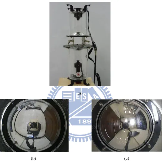
above purpose, we use in this study two catadioptric omni-cameras attached together
in a bottom-to-bottom fashion, forming a two-camera omni-directional imaging
system, as illustrated in Figure 1.1 (a). The two omni-cameras cover respectively the
upper and lower semi-spherical FOV’s simultaneously around the autonomous vehicle,
corresponding to the floor and the ceiling scenes, as shown in Figures 1.1(b) and
1.1(c). In this way, much more room space information can be acquired at a time
without moving the cameras around the entire room space at many spots, which is
necessary when a traditional projective camera is used, to get a full coverage of the
3-D space of the room.
When a vehicle navigates by mopboard following in a room space, the
mopboards used for vehicle guidance may belong to different adjacent walls, and so
the vehicle is likely to get confused in deciding which wall should include an
extracted mopboard edge point. As a result, the vehicle is unable to know the
3
mopboard edge data as done in this study, this problem can be solved. Consequently,
the vehicle not only can make appropriate control of itself, but also can gather desired
environment space data correctly.
(a)
(b) (c)
Figure 1.1 Two catadioptric omni-cameras connected in a bottom-to-bottom fashion into a single two-camera omni-directional imaging system used in this study. (a) The two-camera imaging system. (b) An acquired image of the floor using the lower camera. (c) An acquired image of the ceiling using the upper camera.
After a navigation session is completed, it is desired to construct an indoor
environment map using the collected image information of the walls. Furthermore, it
is also hoped that objects such as doors and windows on the walls can be found out
with their positions estimated. We have also tried to solve these problems in this
4
As a summary, the objective of this study is to design a vision-based automatic
house-layout construction system equipped on an autonomous vehicle system with the
following capabilities:
1. navigating automatically in an unknown indoor room space by mopboard
following;
2. analyzing environment layout information consisting of wall positions
extracted from acquired omni-images;
3. estimating the positions of the windows and doors on the walls;
4. constructing a 3-D space layout of the indoor room space; and
5. drawing a graphic representation of the layout which can be viewed from any
perspective directions and used for simulation of interior design for each
room.
1.2 Survey of Related Studies
To achieve the goal of automatic house-layout construction by vision-based
autonomous vehicle navigation via mopboard following as mentioned previously,
object localization for estimating mopboard positions is required. Various visual
sensing equipments such as cameras and ultrasonic sensors were used to acquire the
3-D information in the vehicle surroundings in the past studies [1-4]. For depth
information estimation, the most common stereo matching method may be used,
which is based on the triangulation principle to obtain the relation between a 3-D
point and multiple cameras, but matching of corresponding points between images is
often a difficult problem in this approach. Use of the laser range finder together with
conventional imaging sensors were also used frequently [5-6]. However, the laser
5
Jeng and Tsai [7] proposed a space-mapping method for the omni-camera image,
which can be used to estimate the location of an object.
In this study, we propose a method which is based on two concepts. The first is
the use of the triangulation principle to measure depths of objects (i.e, their ranges).
The other is the use of the space-mapping technique proposed by Jeng and Tsai [7] to
get the location for a concerned object. In this way, we can estimate the positions of
objects on the floor and walls in a room.
Autonomous vehicles or mobile robots usually suffer from accumulations of
mechanical errors during navigation, which cause inaccurate measures of the moving
distances and orientations yielded by the odometer in the vehicle. Many methods have
been proposed to correct such errors. Chiang and Tsai [8] proposed a method of
vehicle localization by detecting a house corner. Wang and Tsai [9] proposed a
method to correct the position and direction of a vehicle using omni-cameras on a
house ceiling. Chen and Tsai [10] proposed a mechanical error correction method by
curve-fitting the erroneous deviations from correct paths. In this study, we utilize the
curve-fitting method proposed by Chen and Tsai [10] to correct the positions of the
vehicle and use the edge information estimated from images to correct the direction of
the vehicle.
Analyzing the omni-images taken by different types of camera is an important
topic. Kim and Oh [6] proposed a method for extracting vertical lines from an
omni-image with the help of the horizontal lines generated by a laser range finder. Wu
and Tsai [11] proposed a method of approximating distorted circular shapes in
omni-images by ellipses. It is always desired to construct a map for an unknown
indoor environment so that more applications can be implemented. For example,
Biber et al. [12] proposed a method for guiding a robot security guard. They
6
technique to build the 3-D model of an environment. Kang and Szeliski [13] proposed
a method to extract directly 3-D data from images with very wide FOV’s. The goals
of this method are achieved by producing panoramas at each camera location and by
generating scene models from multiple 360° panoramic views. Meguro et al. [14]
presented a motion-stereo device which combines the GPS/DR with omni-directional
cameras to rebuild a 3-D space model. This method provides high precision in
calculating the distance to far-away objects. However, the running time of the stereo
matching process is too long to wait.
1.3 Overview of Proposed System
The goal of this study is to design a system for automatic house-layout
construction in an empty indoor room space using a vision-based autonomous vehicle.
It is assumed that the adjacency walls in the room are perpendicular to each other.
Most houses are of such a type of layout. In order to achieve this goal, the system
needs not only a capability of automatic navigation but also a capability to acquire
environment information automatically. For the vehicle to have such capabilities, an
imaging device with two vertically-aligned omni-cameras connected in a
bottom-to-bottom fashion is designed in this study, which will be described later. With
the environment information collected from the taken images, a method for
constructing a 3-D house layout in graphic form by estimating the locations of
mopboard edges, doors, and windows is also proposed. A rough flowchart of the
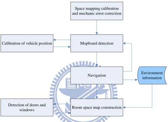
proposed system is illustrated in Figure 1.2.
The system consists of three major phases: setup of the imaging system, vehicle
navigation by mopboard following, and 3-D construction of room space, as described
7
(1) System setup ---
The setup of the system includes space-mapping calibration and mechanic
error correction. For camera calibration, we establish a space-mapping table for
each omni-camera by finding the relations between specific points (on a
specially-designed calibration object) in 2-D omni-images and the corresponding
points in 3-D space. As a result, the vehicle which carries the imaging system has
the abilities to estimate the distances between the vehicle and an object (the
mopboard here) utilizing the omni-images. Mechanic error correction is an
important task because the mechanic errors of an odometer usually will led to
wrong control instructions and inaccurate vehicle localization information. We
also propose a mechanic error correction technique to deal with this problem.
(2) Vehicle navigation by mopboard following ---
Mopboard positions are essential for vehicle navigation in this study.
Therefore, we propose a method to detect mopboard edges from omni-images, and
estimate relative mopboard positions with respect to the vehicle by using the
space-mapping table mentioned above. When the vehicle navigates, the mopboard
edges are also used to adjust the pose of the vehicle to keep its navigation path
parallel to each wall. The vehicle system is designed to record the environment
data during navigation. After the navigation session is completed, a floor-layout
map is created according to the collected mopboard edge data by using a global optimization method for mopboard edge line fitting.
(3) 3-D construction of room space ---
Only creating a floor-layout map is insufficient for use as a 3-D model of the
indoor room space. The objects on walls such as windows and doors must also be
detected and be drawn to appear in the desired 3-D room model. In this study, we
8
on walls in the upper and lower omni-images (taken respectively by the upper
omni-camera and the lower one in the proposed two-camera omni-directional
imaging system), locating them in the 3-D space, and drawing them in the final
3-D room model in a graphic form.
Space mapping calibration and mechanic error correction
Mopboard detection
Navigation
Room space map construction
Environment information Calibration of vehicle position
Detection of doors and windows
Figure 1.2 Flowchart of proposed system.
1.4 Contributions
The major contributions of this study are listed as follows.
1. A technique for finding the focus point of a hyperbolic mirror used in a
process of creating a space-mapping table is proposed.
2. A method for detection of mopboards in omni-images is proposed.
3. A method of using a look-up space-mapping table to estimate the positions
of mopboard edges in omni-images is proposed.
9
edge point correctly to the wall adjacent to the mopboard is proposed.
5. A strategy for vehicle navigation by mopboard following in an unknown
indoor space with a pattern of mutually-perpendicular mopboard edges is
proposed.
6. A global optimization method for constructing an indoor floor-layout map
using extracted mopboard edges is proposed.
7. A method for retrieving accurate 3-D data from different omni-images taken
by the two-camera omni-directional imaging system subject to the
floor-layout map is proposed.
8. Methods for detecting and recognizing the doors as well as windows on
walls from different omni-images are proposed.
1.5 Thesis Organization
The remainder of this thesis is organized as follows. In Chapter 2, the
configuration of the proposed two-camera omni-directional imaging system and the
principle of automatic 3-D house-layout construction are described. In Chapter 3, the
proposed techniques for space-mapping calibration of the omni-cameras and for
mechanic-error correction are described. In Chapter 4, the proposed methods for
mopboard detection and the proposed strategy of vehicle navigation by mopboard
following are presented. In Chapter 5, the proposed methods for room space
construction and analysis of environment data in different omni-images are described.
Experimental results showing the feasibility of the proposed methods are described in
Chapter 6. Conclusions and suggestions for future works are included finally in
10
Chapter 2
Principle of Proposed Automatic 3-D
House-layout Construction and
System Configuration
2.1 Introduction
For indoor 3-D house-layout construction, the use of a vision-based intelligent
autonomous vehicle is a good idea because it can save manpower and the vision
sensors on the vehicle can assist navigation and localization. Besides, the vehicle can
also gather indoor environment information with its mobility.
In the proposed system, we equip the vehicle with two catadioptric
omni-cameras which have larger FOV’s, each covering a half sphere of the 3D space
around the camera. The two omni-cameras are connected and vertically-aligned in a
bottom-to-bottom fashion, form a two-camera imaging device, and are installed on the
vehicle. In such a connected fashion, the imaging system covers the upper and lower
semi-spherical FOV’s simultaneously so that the images of the floor and the ceiling
can be captured simultaneously. With this imaging system, the vehicle can navigate
and collect desired information in indoor rooms. Related control instructions of the
vehicle and communication tools are also developed in this study. The entire system
configuration, including hardware equipments and software, will be described in
Section 2.2.
In order to use the vehicle to carry out the indoor house-layout construction task,
11
turn around, and what kind of information should be collected. When a house agent
wants to use the vehicle to obtain the layout of each empty room in a house in
advance before getting it ready for sale, it is inconvenient to conduct a learning work
to teach the vehicle a navigation path that includes some specific positions as turning
spots. Instead, it is desired that the vehicle can navigate and gather environment
information in an unlearned indoor room space automatically. We will introduce the
main idea of such an automatic 3D house-layout construction process, which we
propose in this study, in Section 2.3. Also, the system must have a process to
transform the collected data into house-layout structure information. In Section 2.4,
we will describe the outline of the proposed process of house-layout construction.
2.2 System Configuration
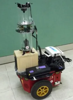
In the proposed vehiclesystem, we make use of a Pioneer 3-DX vehicle made by
MobileRobots Inc. as a test bed. The vehicle is equipped with an imaging system
composed of two omni-directional catadioptric cameras. The imaging system is not
only part of the vehicle system but also plays an important role of gathering
environment information and locating the vehicle. A diagram illustrating the
configuration of this system is shown in Figure 2.1. Because we control the vehicle
system remotely, some wireless communication equipments are necessary. The detail
of the hardware architecture and the used equipments are described in Section 2.2.1.
In order to develop the vehicle system, the software that provides some
commands and control interface is essential for users to control the vehicle and
12
Figure 2.1 Equipment on proposed vehicle system used in this study.
2.2.1 Hardware configuration
The hardware equipments we use in this study include three principal systems ---
the vehicle system, the control system, and the imaging system. In the vehicle system,
the Pioneer 3-DX vehicle itself has a 44cm×38cm×22cm aluminum body with two
19cm wheels and a caster. It can reach a speed of 1.6 meters per second on flat floors,
and climb grades of 25° and sills of 2.5cm. It can carry payloads up to 23 kg. The
payloads include additional batteries and all accessories. By three 12V rechargeable
lead-acid batteries, the vehicle can run 18-24 hours if the batteries are fully charged
initially. An embedded control system in the vehicle allows a user to issue commands
to control the vehicle to move forward or backward and turn around. The system can
also return some status information to the user. Besides, the vehicle is equipped with
an odometer which is used to record the pose and the position of the vehicle. To
control the vehicle remotely, a wireless connection between the user and the vehicle is
necessary. A WiBox is used to communicate with the vehicle by RS-232, so the user
13
The second part is the two-camera imaging device which includes two
catadioptric omni-cameras vertically-aligned and connected in a bottom-to-bottom
fashion, as shown by Figure 2.2(a). The catadioptric omni-camera used in this study is
a combination of a reflective hyperbolic mirror and a CCD camera. Each CCD
camera used in the imaging system is shown in Figure 2.2(b), and a detailed
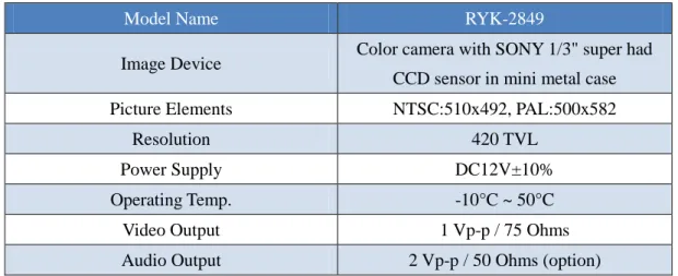
specification about it is included in Table 2.1.
(a) (b)
Figure 2.2 Two catadioptric omni-cameras connected in a bottom-to-bottom fashion into a single two-camera imaging device used in this study. (a) The two-camera device. (b) The CCD camera used in the imaging device.
Table 2.1 Specification of the CCD cameras used in the imaging device.
Model Name RYK-2849
Image Device Color camera with SONY 1/3" super had CCD sensor in mini metal case
Picture Elements NTSC:510x492, PAL:500x582
Resolution 420 TVL
Power Supply DC12V±10%
Operating Temp. -10°C ~ 50°C
Video Output 1 Vp-p / 75 Ohms
14
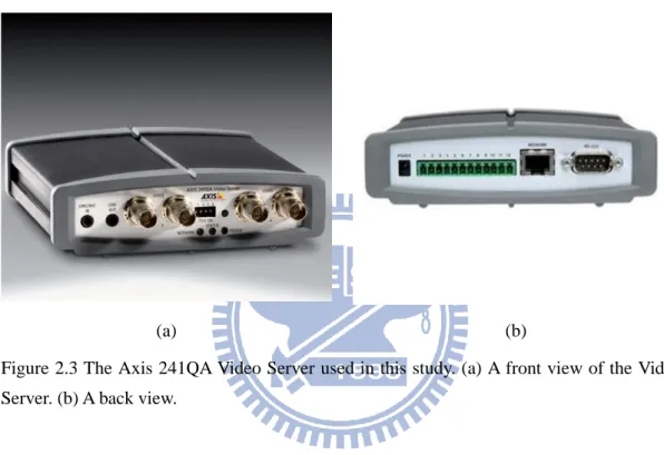
Because the output signals of the CCD cameras used in this study are analog, an
AXIS 241QA Video Server installed in it, as shown in Figure 2.3, has a maximum frame rate of 30 fps. It can convert analog video signals into digital video streams and
send them over an IP network to the main control unit (described next). The imaging
device and the AXIS Video Server are combined into an imaging system.
(a) (b)
Figure 2.3 The Axis 241QA Video Server used in this study. (a) A front view of the Video Server. (b) A back view.
In the control system, a laptop computer is used to run the program developed in
this study. A kernel program can be executed on the laptop to control the vehicle by
issuing commands to it and to conduct processing tasks on captured images. With an
access point, all information between the user and the vehicle can be delivered
through wireless networks (IEEE 802.11b and 802.11g), and captured images can also
be transmitted to users at speeds up to 54 Mbit/s. The entire structure of the vehicle
15
Figure 2.4 Structure of proposed system.
2.2.2 Software configuration
16
Application) for use in this study, which is an API (application programming interface) that assists developers in communicating with the embedded system of the vehicle,
through an RS-232 serial port or a TCP/IP network connection. The ARIA is an
object-oriented toolkit usable under Linux or Win32 OS by the C++ language.
Therefore, we use the Borland C++ builder as the development tool in our
experiments to control the vehicle by the ARIA. The status information of the vehicle
can be obtained by means of the ARIA.
About the AXIS 241QA Video Server, the AXIS Company provides a
development toolkit called AXIS Media Control SDK. Using the Media ActiveX
component from the SDK, we can easily have a preview of the omni-image and
capture the current image data. It is helpful for developers to conduct any task with
the grabbed image.
2.3 Principle of Proposed Automatic
Floor-layout Construction by
Autonomous Vehicle Navigation and
Data Collection
For vehicle navigation in an unknown empty room space, we propose a
navigation strategy based on mopboard following. After a navigation session is
completed, we use the estimated mopboard edge points to construct a floor-layout
map. The main process is shown in Figure 2.5.
In this study, we use a space-mapping technique proposed by Jeng and Tsai [7] to
compute the location of a concerned object using a so-called pano-mapping table.
17
points from omni-images to decide whether or not it has to conduct an adjustment of
its direction to keep its navigation path parallel to each wall. Then, the mopboard edge
points are detected again from the omni-images taken by the imaging system
mentioned previously. By a pattern classification technique, the distance between the
vehicle and each wall can be estimated more accurately, and each extracted mopboard
edge point can be assigned to the wall which contains it. In this way, the vehicle can
estimate the distances between the walls and itself, and know whether to move
forward or turn around. After the navigation session is completed, a floor-layout map
is created according to the collected mopboard edge data by using a global
optimization method for mopboard edge line fitting proposed in this study.
2.4 Outline of Proposed Automatic 3-D
House-layout Construction Process
Only creating a floor-layout map, as described in Section 2.3, is insufficient foruse as a 3-D model of the indoor room space. The objects on walls such as windows
and doors must also be detected and be drawn to appear in the desired 3-D room
model. We have proposed methods for detecting and recognizing the doors as well as
windows on walls in the upper and lower omni-images. The principal steps of the
methods are shown in Figure 2.6.
First, we determine a scanning range with two direction angles for each pair of
omni-images based on the line equation of the floor layout. Because the lower
omni-camera is installed to look downward, it can cover the mopboard on the wall.
We use a pano-mapping table lookup technique to get the scanning radius in the
omni-image by transforming the 3-D space points into corresponding image
18
appropriate 3-D information from different omni-images. Each object which is
detected by the scanning region of each omni-image is regard as an individual one.
Some objects on the wall, such as windows and doors, may appear in the pair of
omni-images (the upper and the lower ones). Therefore, we have to merge the objects
which are detected separately from the upper omni-image and the lower omni-image
according to their positions in order to recognize the doors as well as the windows on
walls. Then, we can locate them in the 3-D space and draw them in the final 3-D room
model in a graphic form.
In summary, the proposed automatic 3-D house-layout construction process
includes the following major steps:
1. automatic floor-layout construction by autonomous vehicle navigation and
data collection as described in Section 2.4;
2. determine a scanning region for each omni-image according to the
floor–layout edges;
3. retrieve information from the scanning region of each omni-image;
4. combine those objects which are detected separately from the upper and
lower omni-cameras according totheir positions;
5. recognize doors and windows from these combined objects;
6. construct the house-layout model with doors and windows on it in a graphic
19
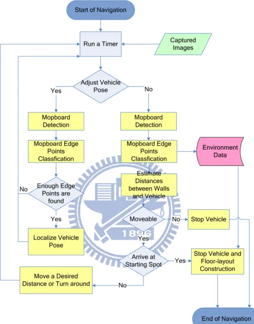
Start of Navigation
Mopboard Detection
Move a Desired Distance or Turn around
Adjust Vehicle Pose Localize Vehicle Pose Mopboard Edge Points Classfication Enough Edge Points are found Mopboard Detection Mopboard Edge Points Classfication Yes No Yes Captured Images Arrive at Starting Spot
Stop Vehicle and Floor-layout Construction End of Navigation No Run a Timer Environment Data Estimate Distances between Walls and Vehicle Moveable Yes No Stop Vehicle Yes No
20
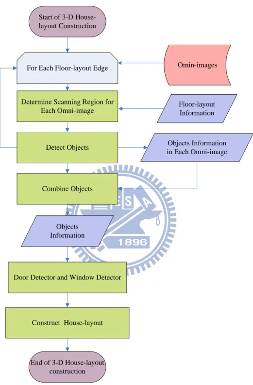
Floor-layout Information Determine Scanning Region for
Each Omni-image
Omin-images
Door Detector and Window Detector Combine Objects
Start of 3-D House-layout Construction
For Each Floor-layout Edge
Objects Information
End of 3-D House-layout construction Construct House-layout
Detect Objects Objects Information in Each Omni-image
21
Chapter 3
Calibration of a Two-camera
Omni-directional Imaging System
and Vehicle Odometer
3.1 Introduction
The vehicle used in this study is equipped with two important devices which are
a two-camera imaging system and a vehicle odometer. We describe the proposed
methods of calibration for these two equipments in this chapter. Before describing the
proposed methods, we introduce the definition of the coordinate system used in this
study in Section 3.1.1 and the relevant coordinate transformation in Section 3.1.2.
The catadioptric omni-camera used in this study is a combination of a reflective
hyperboloidal-shaped mirror and a perspective CCD camera. Both the perspective
CCD camera and the mirror are assumed to be properly set up so that the
omni-camera becomes to be of a single-viewpoint (SVP) configuration. It is also
assumed that the optical axis of the CCD camera coincides with the transverse axis of
the hyperboloidal mirror and that the transverse axis is perpendicular to the mirror
base plane.
For vehicle navigation by mopboard following, the mopboard positions are
essential for vehicle guidance. Besides, these mopboard edge points are very
important for a 3-D house-layout construction. In the proposed system, the vehicle
estimates the distance information by analyzing images captured from the imaging
22
needed. For this purpose, we use a space-mapping technique proposed by Jeng and
Tsai [7] to create a space-mapping table for each omni-camera by finding the relations
between specific points in 2-D omni-images and the corresponding points in 3-D
space. In this way, the conventional task of calculating the projection matrix for
transforming points between 2-D omni-image and 3-D space can be omitted. The
detail about camera calibration is described in Section 3.2.
For vehicle navigation in indoor environments, the vehicle position is the most
important information which is not only used for guiding the vehicle but also as a
local center to transform the estimated positions in the camera coordinate system
(CCS) into the global positions in the global coordinate system (GCS). Though, the
position of the vehicle provided by the odometer of the vehicle may be imprecise
because of the incremental mechanic errors of the odometer. It also results in
deviations from a planned navigation path. Therefore, it is desired to conduct a
calibration task to eliminate the errors. In Section 3.3, we will review the method for
vehicle position calibration which was proposed by Chen and Tsai [10], and a
vision-based calibration method for adjusting the vehicle direction during navigation
will be described in the following chapter.
3.1.1 Coordinate Systems
Four coordinate systems are utilized in this study to describe the relative
locations between the vehicle and the navigation environment. The coordinate
systems are illustrated in Figure 3.1. The definitions of all the coordinate systems are
described in the following.
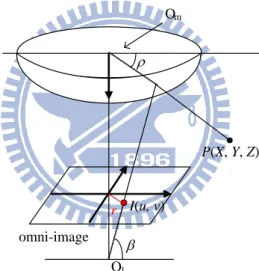
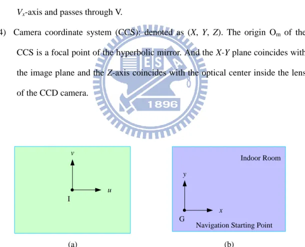
(1) Image coordinate system (ICS): denoted as (u, v). The u-v plane coincides with
23
plane.
(2) Global coordinate system (GCS): denoted as (x, y). The origin G of the GCS is a
pre-defined point on the ground. In this study, we define G as the starting
position of the vehicle navigation by the mopboard following process.
(3) Vehicle coordinate system (VCS): denoted as (Vx, Vy). The Vx-Vy plane is
coincident with the ground. And the origin V is placed at the middle of the line
segment that connects the two contact points of the two driving wheels with the
ground. The Vx-axis of the VCS is parallel to the line segment joining the two
driving wheels and through the origin V. The Vy-axis is perpendicular to the
Vx-axis and passes through V.
(4) Camera coordinate system (CCS): denoted as (X, Y, Z). The origin Om of the
CCS is a focal point of the hyperbolic mirror. And the X-Y plane coincides with
the image plane and the Z-axis coincides with the optical center inside the lens
of the CCD camera. u v I (a) x y G Indoor Room
Navigation Starting Point
(b)
Figure 3.1 The coordinate systems used in this study. (a) The image coordinate system. (b) The vehicle coordinate system. (c) The global coordinate system. (d) The camera coordinate system.
24
(c) (d)
Figure 3.1 The coordinate systems used in this study. (a) The image coordinate system. (b) The vehicle coordinate system. (c) The global coordinate system. (d) The camera coordinate system. (continued)
3.1.2 Coordinate Transformation
In this study, the GCS is determined when starting a navigation session. The
CCS and VCS follow the vehicle during navigation. The relation between the GCS
and the VCS is illustrated in Figure 3.2(a). We assume that (xp, yp) represents the
coordinates of the vehicle in the GCS, and that the relative rotation angle denoted as θ
is the directional angle between the positive direction of the x-axis in the GCS and the
positive direction of the Vx-axis in VCS. The coordinate transformation between the
VCS and the GCS can be described by the following equations:
x = Vx × cosθ - Vy × sinθ + xp; (3.1)
y = Vx × sinθ + Vy × cosθ + yp. (3.2)
The main concept about the relation between the CCS and the ICS is illustrated in
Figure 3.2(b), though the CCS in Figure 3.2(b) is a little different from the CCS in
this study. The relation plays an important role for transforming the camera
25
corresponding image point p. The relation may be described by the following
equations [15-17]: 2 2 2 2 ( )sin 2 tan ( )cos b c bc b c
; (3.3) 2 2 r u v ; (3.4) 2 2 sin f r f
; (3.5) 2 2 cos r r f
; (3.6) 2 2 tan Z c X Y
, (3.7)where a and b are two parameters satisfying the equation of the hyperboloidal mirror
as follows: 2 2 2 2 2 2 2 2 1, , R Z R X Y c a b a b ;
Om and Ol are located at (0, 0, 0) and (0, 0, -c) separately in the CCS; and f is the
focal length of the camera. According to the rotational invariance property of the
omni-camera [17], and by combining with the above equations, we have
2 2 2 2 cos X u X Y u v
; (3.8) 2 2 2 2 sin Y v X Y u v
; (3.9) 2 2 2 2 2 2 2 ( ) ( )( ) 2 ( ) Xf b c u b c Z c bc Z c X Y ; (3.10) 2 2 2 2 2 2 2 ( ) ( )( ) 2 ( ) Yf b c v b c Z c bc Z c X Y , (3.11)26
the corresponding image point p with respect to the u-axis, as shown in Figure 3.2(c).
(a) (b) u v I P(X, Y, Z) p(u, v) θ omni-image plane (c)
Figure 3.2 The relations between different coordinate systems in this study. (a) The relation between the GCS and VCS (b) Omni-camera and image coordinate systems [11]. (c) Top view of (b).
3.2 Calibration of Omni-directional
Cameras
27
is indispensible. However, the conventional calibration method is complicated for
calculating intrinsic and extrinsic parameters. An alternative way is to use the
space-mapping technique to estimate the relation between points in the 2-D image plane and 3-D space and to establish a space-mapping table for it [7]. The detailed
process is reviewed in Section 3.2.2. In the process of establishing the space-mapping
table, the information about the focal location of the hyperboloidal mirror is important
because the focal point is taken to be the origin in the CCS. The process to find the
focal point of the hyperboloidal mirror is described in Section 3.2.1.
3.2.1 Proposed Technique for Finding Focal Point of
Hyperboloidal Mirror
In order to creating the space-mapping table, it is indispensible to select some
pairs of world space points with known positions and the corresponding points in the
omni-images. Note that an image point p is formed by any of the world space points
which all lie on the incoming ray R, as shown in Figure 3.3, where we suppose that
Om is the focal point of the hyperboloidal mirror, Ow is on the transverse axis of the
hyperboloidal mirror, and P1 and P2 are two space points on the ray R. Besides, we
also assume that the corresponding image point is p .Subsequently, we have the
corresponding point pairs (P1, p) and (P2, p) which then are used to create the table.
However, if we take Ow as the focal point, as a result P1 and P2 will lie on different
light rays, though the corresponding image points are still p. In this way, the incorrect
pairs will result in an incorrect space-mapping table. To provide accurate pairs, we
28
Figure 3.3 The space points and their corresponding image points.
To find out the focal point of the hyperboloidal mirror, as shown in Figure 3.4,
we use two different landmarks L1 and L2 which have the same corresponding image
point p with known heights and horizontal distances from the transverse axis of the
hyperboloidal mirror. We assume that Ow is at (0, 0, 0). Then, according to the
involved geometry shown in Figure 3.4, the position of the focal point can be
computed by the following equations:
1 2 1 1 2 1 tan H O Om w H H D D D
; (3.12) 2 1 1 1 1 1 2 1 tan m w H H O O H D H D D D
. (3.13)29
3.2.2 Review of Adopted Camera Calibration
Method
Jeng and Tsai [7] proposed a space-mapping method to estimate the relation
between points in the 2-D image plane and the 3-D space and to establish a
space-mapping table. By observing Figure 3.2(b) and Eq. (3.3) through (3.7), it is
noted that there exists a one-to-one relation between the elevation angle α and the
radial distance r. By using the space-mapping table as well as according to the
rotational invariance property, we can know the relative elevations and directions of
the concerned targets in images.
The adopted method [7] includes three major procedures: landmark learning,
estimation of coefficients of a radial stretching function, and space-mapping table
creation, as described respectively in the following.
(1) Landmark learning ---
We select some landmark point pairs of world space points with known positions
and their corresponding pixels in a taken omni-image. More specifically, the
coordinates of the landmark points are measured manually with respect to a selected
origin in the CCS. In this study, the origin in the CCS is a focal point of the
hyperboloidal mirror which can be found as described in Section 3.2.1. As shown in
Figure 3.5, we selected n landmark points on the omni-image, and recorded the pairs
of the space coordinates (Xk, Yk, Zk) and the image coordinates (uk, vk), where k =0,
1,…, n 1.
(2) Estimation of coefficients of radial stretching function ---
As shown in Figure 3.6, the same elevation angles correspond to the same radial
distances. Therefore, the radial distance r from each image pixel p with (u, v) in the
30
attempt to describe the function fr(ρ), called a radial stretching function, by the following 5th-degree polynomial function:
1 2 3 4 5
0 1 2 3 4 5
( )
r
r f
a a
a
a
a
a
, (3.14)where a0 to a5 can be estimated using the landmark point pairs, as described in the
following major steps [7].
selected landmark point
O
cFigure 3.5 The interface for selecting landmark points.
Step 1. Elevation angle and radial distance calculation ---
Use the selected landmark point pair (Pk, pk), including the coordinates (Xk, Yk, Zk)
in the CCS and the coordinates (uk, vk) in the ICS, to calculate the elevation angle ρk
of Pk, in the CCS and the radial distance rk of pk in the ICS by the following
equations: 1 tan ( k) k k Z D
, (3.15) 2 2 k k k r u v , (3.16)31
Om of the mirror.
Step 2. Calculation of coefficients of the radial stretching function ---
Substitute all pairs (ρk, rk), where k=0, 1, …, n 1, into Eq. (3.14) to get n homogeneous equations as follows:
1 2 3 4 5 0 0 0 1 0 2 0 3 0 4 0 5 0 1 2 3 4 5 1 1 0 1 1 2 1 3 1 4 1 5 1 1 2 3 4 5 1 1 0 1 1 2 1 3 1 4 1 5 1 ( ) , ( ) , ( ) . r r n r n n n n n n r f a a a a a a r f a a a a a a r f a a a a a a
, (3.17)and solve them to get the coefficients (a0, a1, a2, a3, a4, a5) of the function fr(ρ).
Om P(X, Y, Z) I(u, v) omni-image Ol r
Figure 3.6 Illustration of the relation between radial r in ICS and elevation ρ in CCS.
Step 3. Space-mapping table creation ---
The space-mapping table to be constructed is a 2-dimensional table with
horizontal and vertical axes specifying respectively, the range of the azimuth angle θ
as well as that of the elevation angel ρ of all possible incident light rays going through
the focal point of the mirror.
Table 3.1 shows an example of the pano-mapping table of size M×N. Each entry
32
which represents an infinite set Sij of points in the CCS passing through by the light
ray with azimuth angel θi and elevation angle ρj. And for the reason that these world
space points in Sij are all projected onto the identical pixel pij in any omni-image taken
by the camera, a mapping relation between Sij and pij as shown in Figure 3.7 can be
derived. The mapping table shown in Table 3.1 is constructed by filling entry Eij with
coordinates (uij, vij) of pixel pij in the omni-image.
Table 3.1 Example of pano-mapping table of size M×N [7].
Figure 3.7 Mapping between pano-mapping table and omni-image [7] (or space-mapping table in this study).
More specifically, the process of filling entries of the pano-mapping table can be
summarized by the following major steps [7].
Step 1. Divide the range 2π of azimuth angles into M intervals and compute θi by
(2 / ), for 0,1,..., 1
i i M i M
33
Step 2. Divide the range [ρe, ρs] of the elevation angles into N intervals and compute ρj
by
[( ) / ] , for 0,1,..., 1
j j e s N s j N
. (3.19)Step 3. Fill the entry Eij with corresponding image coordinates (uij, vij) by
cos ; sin , ij j i ij j i u r v r
(3.20) where rj is computed by 1 2 3 4 5 0 1 2 3 4 5 ( ) j r j j j j j j r f
a a
a
a
a
a
(3.21)with the coefficients (a0, a1, a2, a3, a4, a5) computed above.
After establishing the space-mapping table, we can determine the elevation and
azimuth angle of a space point by looking up the table.
3.3 Calibration of Vehicle Odometer
Autonomous vehicles or mobile robots usually suffer from accumulations ofmechanical errors during navigation. The vehicle we used in this study has been found
to have a defect of this kind that when it moves forward, the vehicle deviates leftward
from the original path gradually, and the position and the direction angle of the
vehicle provided by the odometer are different from the real position and direction
angle of the vehicle. Because the mechanic errors of an odometer usually will lead to
wrong control instructions and inaccurate vehicle localization information, it is
desired to conduct a calibration task to eliminate such errors.
34
curve-fitting the erroneous deviations from correct paths. In this study, we use this
method for correcting the vehicle odometer readings. In Section 3.3.1, we describe
how we find out the deviation values in different distances and build an odometer
calibration model for them. In Section 3.3.2, we will derive an odometer reading
correction equation by a curve fitting technique. Finally, the use of such error
correction results is described in Section 3.3.3.
3.3.1 Odometer Calibration Model
In this section, first we describe an experiment we conducted to record the
vehicle’s deviations from a planned navigation path at different distances from a navigation starting point. We attach a stick on the frontal of vehicle and let it point to
the ground in such a way that the stick is perpendicular to not only the Vy-axis in the
VCS but also the ground. The stick and the two contact points of the two driving
wheels with the ground are used to find out the origin of the VCS. The equipments
used in this experiment were a measuring tape, two laser levelers, and the autonomous
vehicle. We chose a point from the crossing points formed by the boundaries of the
rectangular-shaped tiles on the floor, as the initial position O of vehicle navigation;
and mark the positions by pasting a sticky tape on the ground. Also, we designated a
straight line L along the tile boundaries from O.
First, we used the two laser levelers to adjust the position of the vehicle by hand
such that the two contact points of the two driving wheels with the ground lie on the
boundaries of the tiles and that the stick on the vehicle is perpendicular to L. Second,
we drove the vehicle forward for a desired distance on a straight line L. Third, we
marked the terminal position T reached by the vehicle by finding out the origin in the
35
repeated the steps at least five times for each desired distance. An illustration of the
experiment is shown in Figure 3.8, a detailed algorithm for the process is described in
the following, and the experimental results are shown in Table 3.2.
Figure 3.8 Illustration of the experiment.
Algorithm 3.1. Building a calibration model of the odometer.
Input: none
Output: A calibration model of the odometer. Steps:
Step 1. Choose an initial point O from the crossing points of the boundaries of
the rectangular-shaped tiles on the floor, and designate a straight line L
which starts at O and coincides with some of the tile boundaries.
Step 2. Use the laser levelers to check if the two contact points of the two driving
wheels with the ground lie on the boundaries; and if not, adjust vehicle
36
Step 3. Drive the vehicle to move forward until it arrives at a desired distance on
a straight line L.
Step 4. Mark the terminal position T reached by the vehicle.
Step 5. Measure the distance between T and L.
Step 6. Repeat Steps 2 through 5 at least five times for each desired moving
distance and record the results.
Table 3.2 The results of the experiment of building an odometer calibration model.
Move Distance (cm) Average Distance of Deviation (cm)
30 0.31 40 0.41 50 0.83 60 0.88 70 0.93 80 1.38 90 1.93 100 2.14 110 2.55 120 2.70 130 2.90 140 3.2 150 3.32
3.3.2 Curve Fitting
The distribution of the deviations of the experimental results in Section 3.3.1 is
shown in Figure 3.9. We found out that the distribution of the data can be described as
a curve as a mechanical-error calibration model for the vehicle. Therefore, we use the
least-squares-error (LSE) curve fitting technique to obtain a third-order equation to fit
these data. After that, we can use the derived curve equation to calibrate the vehicle
37 0 0.5 1 1.5 2 2.5 3 3.5 4 0 50 100 150 200 Move Distance (cm) A ver ag e D is tan ce o f D ev iat io n (cm )
Figure 3.9 The distribution of the deviations.
The principle of the curve fitting technique we adopt can be explained as follows.
We consider a polynomial function L of degree k:
0 1
: ... k
k
L y a a x a x . (3.22)
And with the pairs of measured data, (x1, y1), (x2, y2), …, (xn, yn) mentioned above, we can use the LSE principle to fit the pairs by
2 0 1 1 [ ( ... )] n k i i k i i E y a a x a x
. (3.23)The partial derivatives of E with respect to a0, a1, …, and ak, respectively, are
0 1 1 2 [ ( ... )] 0, 0,1, ..., n k i i k i i t t E y y a a x a x t n a a
. (3.24)From Eq. (3.24), we can derive a relation matrix as follows:
1 1 1 1 0 2 1 1 1 1 1 1 1 2 1 1 1 1 ... ... ... n n n k i i i i i n n n n k i i i i i i i i i k n n n n k k k k i i i i i i i i i n x x y a a x x x x y a x x x x y
![Figure 3.2 The relations between different coordinate systems in this study. (a) The relation between the GCS and VCS (b) Omni-camera and image coordinate systems [11]](https://thumb-ap.123doks.com/thumbv2/9libinfo/8245370.171493/38.892.166.726.205.891/figure-relations-different-coordinate-systems-relation-coordinate-systems.webp)