利用次通道降峰法以降低正交分頻多工系統的峰均比

(1)

國

立

交

通

大

學

電

機

與

控

制

工

程

學

系

碩

士

論

文

利用次通道降峰法以降低正交分頻多工

系統的峰均比

PAPR Reduction for OFDM Systems

Using Subchannel Peak Reduction

研究生 : 吳芳儀

指導教授 : 林源倍博士

(2)

PAPR Reduction for OFDM

Systems Using Subchannel Peak

Reduction

Student : Fang-Yi Wu

Advisor : Yuan-Pei Lin

Department of Electrical and Control Engineering

National Chiao Tung University

Abstract

Recently there has been great interest in the Orthogonal Fre-quency Division Multiplexing (OFDM) systems. However one dis-advantage of OFDM systems is high peak-to-average power ratio (PAPR). In this thesis, we will propose a new method called Sub-channel Peak Reduction (SPR). The symbols of a few selected sub-channels are chosen to multiple a rotation individually so that PAPR is reduced. Transmission rate is slightly lower. However, no side in-formation bit is needed. The optimal solution of the rotation can be found by exhaustive search (SPR-ES). We will propose an iterative ap-proach method (SPR-IT) to find suboptimal rotating for the selected subchannels. SPR-IT can have lower complexity than SPR-ES. Sim-ulation results shows SPR-ES and SPR-IT can efficiently reduce the peak value of the transmitted signal. The simulations will demon-strate that our method provide a nice tradeoff between bit rate and

(3)

2.1 The OFDM systems model . . . 5 2.2 The PAPR of OFDM systems . . . 6 3 PAPR Reduction By Tone Injection [6] 9 3.1 Tone Injection for Real Multicarrier Systems . . . 9 3.2 Tone Injection for passband communications . . . 15 4 The Subchannel Peak Reduction Method 19 4.1 An Exhaustive Search Scheme . . . 20 4.2 An Iterative Approach Method . . . 25 5 Computational Complexity 30 5.1 Exhaustive Search . . . 30 5.2 Iterative Approach . . . 34 5.3 Tone Injection (for passband communication) . . . 35 6 Simulation Results 39

(4)

List of Figures

2.1 The OFDM system. . . 5 2.2 The transmitter of OFDM systems. . . 6 2.3 An example figure. a1 has better PAPR performance than a2. . . 8 3.1 16 QAM constellation and its Gray code mapping. . . 10 3.2 A example of a point A mapped to another 8 points. . . 11 3.3 9 × 16 QAM constellation. . . . 12 3.4 The transmitter plus tone injection method of the OFDM system. 14 3.5 The marked horizontal and vertical axes of 16QAM. . . 16 3.6 The expanded 16 QAM constellation can be divided into three

groups, original 16 QAM, part A, and part B. . . 17 4.1 An example of bits-to-symbol mapping for PR subchannel when

the constellation is 16 QAM. (a) The symbols on the PR subchan-nels may be rotated by multiples of 180◦_{. (b) The symbol can be}

rotated by multiples of 90◦_{. . . .} ₂₀

4.2 The block diagram of SPR method . . . 21 4.3 Example 4.1. SPR-ES: 2, 4, 8 PR subchannels and rotation

factors are selected from {+1, −1}. . . . 23 4.4 Example 4.2. SPR-ES: 2, 4 PR subchannels and rotation factors

are selected from {+1, −1, +j, −j}. . . . 24 4.5 The block diagram of Iterative Approach method. . . 25 4.6 Example 4.3. SPR-IT: 2, 4, 8 PR subchannels and rotation

(5)

4.7 Example 4.4. SPR-IT: 2, 4 PR subchannels and rotation factors are selected from {+1, −1, +j, −j}. . . . 28 4.8 Example 4.5. SPR-ES v.s SPR-IT. 8 PR subchannels and

rota-tion factors selected are from {+1, −1}. . . . 29 5.1 SPR-ES. (a) The IDFT block can put in front of the adder. (b)

The M-point IDFT can be replaced by the P-point IDFT. . . 31 6.1 The OFDM system with SPR method. . . 40 6.2 A clipping with maximum amplitude A. . . . 40 6.3 BER. N0=1. SPR-ES uses 8 PR subchannels and rotation factors

are selected from {+1, −1} and tone injection. . . . 42 6.4 PAPR. N0=1, BER=10−3. SPR-ES uses 8 PR subchannels and

rotation factors are selected from {+1, −1} and tone injection. . 42 6.5 BER. Fixed average transmission power. P0 = 10.

SPR-ES uses 8 PR subchannels and rotation factors are selected from

{+1, −1} and tone injection. . . . 43 6.6 BER. Fixed average transmission power and the clipping

ratio. (P0 = 10, γ = 2). SPR-ES uses 8 PR subchannels and

rotation factors are selected from {+1, −1} and tone injection. . 44 6.7 BER. Fixed average transmission power and the clipping

ratio. (P0 = 10, γ = 3). SPR-ES uses 8 PR subchannels and

(6)

List of Tables

5.1 Complexity Comparison of the SPR-ES, SPR-IT, and Tone Injec-tion methods. If P ∈ {0,M

4 − 1,M2 − 1,3M4 − 1} , the complex

multiplication of SPR-IT (n=2) and SPR-IT (n=4) are zero. . . 37 5.2 Example 5.1. Complexity comparison of the SPR-ES, SPR-IT,

and tone injection methods. 8 PR subchannels are selected for SPR-ES and SPR-IT and the rotation factors are selected from

(7)

Chapter 1 Introduction

Orthogonal frequency division multiplexing (OFDM) [1] is a multicarrier modu-lation technique that has been used for many applications, such as wireless local area networks (WLANs) [2], digital video broadcasting (DVB) [3], and digital audio broadcasting (DAB) [4]. International standards making use of OFDM for high speed wireless communications are already established or being established by IEEE 802.11, IEEE 802.16, IEEE 802.20, and European Telecommunications Standards Institute (ETST) Broadcast Radio Access Network (BRAN) commit-tees.

In OFDM systems, the input bit stream is coded as modulation symbols, e.g., quadrature amplitude modulation (QAM). The channel is divided into sub-channels, each with a different frequency band. Modulation symbols of different subchannels carry the same number of bits because there is usually no bit/ power allocation in OFDM systems. The transmitter and receiver performance inverse Discrete Fourior Transform (IDFT) and Discrete Fourior Transform (DFT) com-putations respectively. At the transmitter, for each block, a certain redundancy known as cyclic prefix (CP) [5] is added. When the channel order is not large than the prefix length, inter block interference (IBI) can be easily removed by discarding the prefix at the receiver. The OFDM system is attractive because of its high-bit-rate transmission. However, an OFDM signal may have high peak to average power ratio (PAPR) at the transmitter which causes the power amplifier of the transmitter to operate in a low efficiency region [6]. How to reduce the

(8)

PAPR is an important issue in the design of transmitters.

Many schemes have been proposed to reduce the PAPR. One method is called clipping [7], which limits the peak envelope of the input signal to a desired maxi-mum value. The clipping process is nonlinear and may causes in-band distortion and out-of-band radiation. Coding method in [8]-[10] are proposed to reduce PAPR by selecting some codewords with lower PAPR for transmission. Such coding techniques require large lookup tables for encoding and decoding. There-fore, it is fit for systems with a small number of subcarriers. The selective map-ping (SLM) [11][12] and partial transmit sequence (PTS) [13] can efficiently lower the peak power of the OFDM transmitted signal. In the SLM approach, after multiplying some phase sequences to the input signal to generate different candi-date signals, we can choose the one with the least PAPR to transmit. In the PTS method, the input sequence is divided into disjoint subblocks. Optimally combin-ing those disjoint subblocks and phase factors can have a lower PAPR sequence. Both SLM and PTS need to send side information to express how the signal was produced. In the OFDM systems, blocks are grouped and sent in packets. The side information for PAPR reduction is transmitted as part of the preamble. The transmitter needs to generate all the blocks before the side information for PAPR is determined and encoded in the preamble. This leads to a higher complexity for the transmitter. If the decoder makes error then the receiver will not know how the transmitted signal is related to the original signal before using PAPR reduc-tion method. Besides, the processes of SLM and PTS increase the computareduc-tional complexity. The SLM method needs m M-point IDFT to generate m candidates. The PTS scheme needs (log₄m + 1) M-point IDFT to generate m candidates

when the rotation factors are chosen from {±1, ±j}. [14]-[16] are proposed at the cost of a minus performance degradation. Tone injection can reduce PAPR by increasing the constellation size. Then the points in the original constellation can be mapped into several equivalent points. The expanded constellation needs more transmission power.

(9)

computa-We choose a few subchannels as peak reduction (PR) subchannels. The symbols of the PR subchannels are chosen for the purpose of the PAPR reduction. The symbols of the PR subchannels may be rotated by multiplies of 180◦ _{or multiplies}

of 90◦ _{individually. For 180}◦_{-rotation case, if b bit constellation are used for all}

subchannels, on the PR subchannel there are (b−1) bits can be transmitted. Bits are coded to symbol as usual on the non PR subchannel. For the decoder, the received symbol and its rotated by multiplies of 180◦ _{symbol are mapped to the}

same bits. In SPR method, by exhausting all possible combinations of rotations for the PR subchannel we can found the smallest PAPR. The solution is optimal and it is exhaustive search of the SPR method. We call it SPR-ES. The com-plexity can be reduced using a suboptimal rotation of the PR subchannel. It can be done by iterating PR subchannels one by one. The scheme is called SPR-IT and the PAPR performance is close to that of SPR-ES. SPR will decrease the transmission rate slightly. SPR provide a tradeoff between bit rate and PAPR reduction. However, no side information bit is needed.

1.1 Outline

• Chapter 2: The basic structure of OFDM systems and the PAPR of OFDM

systems are presented. The common performance measure for PAPR re-duction techniques will also be mentioned.

• Chapter 3: We will introduce two cases of tone injection method which was

proposed by J. Tellado [6]. One used on real multicarrier systems and the other is for passband communication.

• Chapter 4: New method called Subchannel Peak Reduction will be proposed

in this chapter. In section 4.1, we will see Exhaustive Search method. Iterative Approach scheme will be discused in section 4.2.

• Chapter 5: The calculations of complexity for Exhaustive Search, Iterative

(10)

• Chapter 6: Some computer simulation results about PAPR and BER will

be seen and the computational complexity comparison are also put in this chapter.

• Chapter 7: Conclusion is given in chapter 7.

1.2 Notations

1. Bold faced upper-case letters are used to represent matrices and bold faced lower-case letters are used to represent vectors.

2. A† _{denotes transpose-conjugate of A.}

3. AT _{denotes transpose of A.}

4. The function E[x] denotes the average value or expect value of x.

5. The element-wise multiplication of a M × 1 vector g and a M × 1 vector f is a M × 1 vector given by:

g . × f =      g0f0 g1f1 ... gM −1fM −1      M ×1 .

6. The notation WM is used to represent the normalized M × M DFT matrix

given by [WM]kn = 1 √ Me −j2π Mkn, where 0 ≤ k, n ≤ M − 1.

(11)

Chapter 2 OFDM systems

2.1 The OFDM systems model

M-point IDFT P/S_(M) _CP _channel noise discard CP S/P (M) M-point DFT s0 s1 s_M à1 s

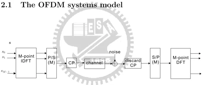
Figure 2.1: The OFDM system.

Fig. 2.1 is the block diagram of the OFDM system. The input symbol block s is a M × 1 vector, s = [s0, s1, · · ·, sM −1]T, where M is the number of subchannels.

The element skin s represents the modulation symbol of the k-th subcarrier. The

input symbol block passes through the M-point IDFT and the parallel to serial conversion (P/S) gets serial sample train. For every block of M data samples, the transmitter adds a cyclic prefix (CP) of length ν samples of the transmitted blocks. After CP process, the transmitted block of M + ν samples pass through the channel plus noise. With a proper insertion of CP, an FIR channel can be decomposed into M parallel AGN subchannels with a gain that depends on the channel. The efficiency of the transceiver is M _{, the larger the channel order is,}

(12)

the larger the cyclic prefix is needed to eliminate ISI, and the lower the efficiency is. When the channel is additive white Gaussian noise (AWGN) channel, there is no inter symbol interference (ISI) and the transmission error comes from the channel noise only. At the receiver, after discarding the cyclic prefix called discard CP and serial to parallel (S/P) conversion gets the parallel samples. The DFT matrix is applied to the received parallel samples

In this thesis, we assume the channel order is not large than the prefix length

ν so there is no IBI. For transmission, We can only consider an input block and

an output block, ie., one-shot transmission.

2.2 The PAPR of OFDM systems

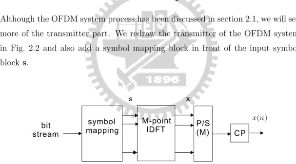
Although the OFDM system process has been discussed in section 2.1, we will see more of the transmitter part. We redraw the transmitter of the OFDM system in Fig. 2.2 and also add a symbol mapping block in front of the input symbol block s. M-point IDFT P/S_(M) _CP symbol mapping x s x(n) bit stream

Figure 2.2: The transmitter of OFDM systems.

The bit stream consists of 00_{s and 1}0_{s. The symbol mapping block takes}

several bits of the bit stream and maps these bits to a real or complex symbol. The sequence x is generated by s and a normalized M × M IDFT matrix W†,

(13)

where W†₌ _√1 M      1 1 . . . 1 1 W . . . WM −1 ... ... . .. ... 1 WM −1 _{. . . W}(M −1)2      † , and W = e−j2π

M. The m-th subcarrier in x can be expressed as

xm = 1 √ M M −1_X k=0 skej2πkm/M, 0 ≤ m ≤ M − 1. (2.2)

In Fig. 2.2, x(n) is the transmitter output signal which is obtained by x passing through parallel to serial conversion and cyclic prefix operation. The PAPR of OFDM signal x(n) is defined as

PAPR = maxn| x(n) |

2

E[| x(n) |2_] , (2.3)

where E[·] denotes the expectation operator. The parallel to serial conversion is to convert a set of parallel input data x to a serial stream. The cyclic prefix is to copy the last fewer samples at the end of each block and place them at the beginning. Both operations do not change the maximum value of x, so the peak power do not change after these two processes. When the symbol mapping is decided, the average power is fixed. From above, we can find that x(n) has the same peak power and the same average power as the IDFT output vector x, therefore we can consider PAPR as the following equation instead,

PAPR = maxm | xm |

2

E[| xm |2]

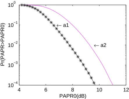
. (2.4) The cumulative distribution function (CDF) of the PAPR is one of the most frequently used performance measure for PAPR reduction techniques. In this the-sis, the complementary cumulative distribution function (CCDF) is used instead of the CDF. The CCDF of the PAPR denotes the probability that the PAPR of a data block exceeds a given threshold (PAPR0). CCDF is defined as:

(14)

The horizontal and vertical axes represent the threshold for the PAPR and the probability that the PAPR of a data block exceeds the threshold respectively. In Fig. 2.3, for PAPR thresholds, if a curve a1 has smaller horizontal values than the other curve a2, a1 has better PAPR performance than a2. From this phenomenon, the closer the CCDF is to the vertical axis, the better its PAPR characteristic is. 4 6 8 10 12 10−4 10−3 10−2 10−1 100 PAPR0(dB) Pr(PAPR>PAPR0) ← a1 ← a2

(15)

Chapter 3 PAPR Reduction By Tone

Injection [6]

In this chapter, we will briefly introduce the tone injection method which was proposed by J. Tellado [6]. In section 3.1, the usage of tone injection method for Real Multicarrier systems will be discussed. We will see this method using for passband communications in section 3.2.

3.1 Tone Injection for Real Multicarrier

Sys-tems

The basic idea of tone injection method is to let each of the point in the original basic constellation to map into several equivalent points in the expanded constel-lation. The above demand can be done by increasing the constellation size and it is equivalent to injecting a tone of the appropriate frequency and phase in the multicarrier symbol.

Assume a 2b _{QAM (b-bit QAM) is used as a modulation scheme and the}

min-imum distance between constellation points is d. Let sk be the k-th modulation

symbol of the input block obtained by mapping b bits to the 2b _QAM

constel-lation. The real part of sk is Rk and the imaginary part is Ik. Both Rk and Ik

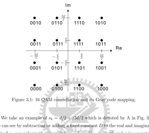
can take values from {±d/2, ±3d/2, · · · , ±(√2b_{− 1)d/2}. Now consider 16 QAM}

(16)

2 d 2 d à2 d à2 d à 2 3 d à 2 3 d 2 3 d 2 3 d 0000 0100 1100 1000 0001 0101 1101 1001 0011 0111 1111 1011 0010 0110 1110 1010 Re Im

Figure 3.1: 16 QAM constellation and its Gray code mapping.

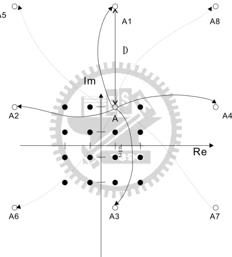
We take an example of sk = d/2 + j3d/2 which is denoted by A in Fig. 3.2.

We can see by subtracting or adding a fixed constant D to the real and imaginary part of sk can enlarge the constellation, where D = a · d

√

2b _{and a is a constant}

which is selected as a ≥ 1. D is a real constant known by the transmitter and receiver. The original sk can become

¯

sk = sk+ pkD + jqkD (3.1)

= (Rk+ pkD) + j(Ik+ qkD), (3.2)

where pk and qk are integers and they can take values from {+1, −1, 0}. After

picking pk and qk, point A can expand to another 8 points: A1 to A8. Every

point on the original 16 QAM constellation can be expanded to another 8 points like the above example. If D is chosen in the special case where a = 1, and

D is d√2b_{, then the expanded constellation becomes a lattice (equally spaced}

points) [Kschischang et al., 1998a, Kschischang et al., 1998b,]. The expanded constellation is equivalent to a 9 × 16 QAM constellation which is in Fig. 3.3.

(17)

2 d

Re

Im

D

A8 A7 A2 A3 A A5 A4 A1 A6

(18)

Re Im

d D

(19)

In order to generate the real transmitted signals, the number of IDFT must be even and the input symbol block s has to be conjugate symmetric,

sk = ½ s∗ M −k, otherwise 0, k = 0,M 2 . (3.3) The element of transmitted IDFT output x can be written as

xn = 1 √ M M −1_X k=0 skej2πkn/M, 0 ≤ n ≤ M − 1 (3.4) = √2 M M 2−1 X k=0 skej2πkn/M. (3.5) Let sk = Rk+ jIk, xn = 2 √ M M 2−1 X k=0 (Rk+ jIk)ej2πkn/M (3.6) = √2 M M 2−1 X k=0 [Rkcos( 2πkn M ) − Iksin( 2πkn M )]. (3.7)

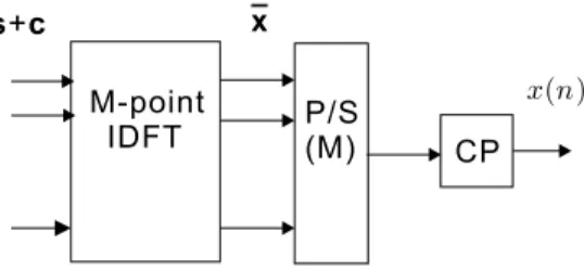
Using tone injection process is equivalent to adding a M × 1 vector c to s, where ck = pkD + jqkD. This means that the input block s becomes s + c which

is in Fig. 3.4. IDFT is applied and the output is x. xn is the n-th subchannel of

x and can be formulated as

xn = 1 √ M M −1_X k=0 ¯ skej2πkn/M (3.8) = √1 M M −1_X k=0 (sk+ ck)ej2πkn/M, 0 ≤ n ≤ M − 1. (3.9)

Because D is known at the receiver, ckcan be removed at the receiver by applying

(20)

M-point

IDFT P/S_(M) _CP

x s+c

x(n)

Figure 3.4: The transmitter plus tone injection method of the OFDM system. For a real multicarrier system, assume xn0 has the maximum value and xn0 >

0. We can modify the n0-th subchannel by tone injection method per dimension.

It means that the real or imaginary part can be changed. Here we used tone injection scheme on the real dimension. Assume cos(2πk0n0

M ) = l, l > 0 for a

frequency k0. The real part of k0-th subchannel is going to be modified.

xn0 = 2 √ M PM 2−1 k=0 [Rkcos(2πkn_M 0) − Iksin(2πkn_M 0)] = _√2 M PM 2−1 k=0,k6=k0[Rkcos( 2πkn0 M ) − Iksin( 2πkn0 M )] + _√2 M[Rk0cos( 2πk0n0 M ) − Ik0sin( 2πk0n0 M )]. (3.10) We subtract Rk0 by D, xn0 becomes ¯xn0: ¯ xn0 = 2 √ M PM 2−1 k=0,k6=k0[Rkcos( 2πkn0 M ) − Iksin( 2πkn0 M )] + _√2 M[(Rk0 − D) cos( 2πk0n0 M ) − Ik0sin( 2πk0n0 M )] = xn0 − 2 √ MD cos( 2πk0n0 M ). (3.11)

We can see that in (3.11) xn0 > 0 also both D and cos(

2πk0n0

M ) are positive, so ¯xn0

is smaller than xn0. This is meant that the peak reduction is

2

√

MD cos(

2πk0n0

M ). A

similar argument follows for other permutations, for example when cos(2πk0n0 M ) <

0, we can add D to Rk0 in order to lower ¯xn0. These ideas can also extend to

sin(2πkn0

(21)

for each subchannel k0. The general equation can be expressed as following, ¯ xn = xn+ 2 √ M(±D){cos, sin}( 2πk0n M ), n = 0, 1, · · · , M − 1. (3.12)

3.2 Tone Injection for passband communications

The tone injection method for real multicarrier systems proposed by J. Tellado [6] was introduced in Section 3.1. For passband communication, we now extend this method to complex case.

For passband communication systems, because the values of IDFT output are complex, there is no restriction on the input symbols. Complex values can not compare with zero. Therefore, every input modulation symbol for each block needs to modify. The modification is the same as that section 3.1: expand the original 16 QAM constellation to a 9 × 16 QAM by adding or subtracting a constant D to the real and imaginary part of the subchannel, where D is d√2b_.

After all the subchannels doing all the same modifications, find the sequence with the smallest PAPR. D is decided at first and both the transmitter and the receiver know the value. Using a modulo-D process can map the received signals back to the original constellation. Therefore, there is no bit lost to transform side information from the transmitter to the receiver. The expanded constellation will cause bigger transmission power. This will be discussed in the next paragraph.

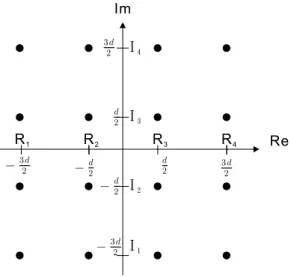
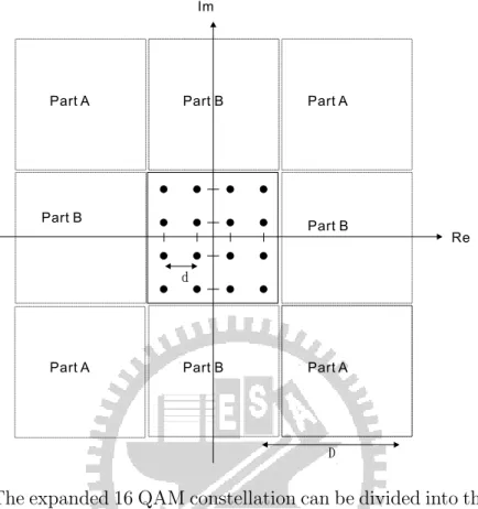
We mark the horizontal and vertical axes as Fig. 3.5. Assume the all constel-lation points are equiprobable. The average energy εsof modulation symbols can

be written as εs = 4 16[ 4 X k=1 Rk2+ 4 X k=1 Ik2] (3.13) = 4 16[R1 2_{+ R} 22+ R32+ R42+ I12+ I22 + I32+ I42] (3.14) = 2 × 4 16[( −3d 2 ) 2_{+ (}−d 2 ) 2_{+ (}d 2) 2_{+ (}3d 2 ) 2_] _(3.15) = 10 4 d 2_. _(3.16)

(22)

2 d 2 d à2 d à2 d à 2 3 d à 2 3 d 2 3 d 2 3 d Re Im R1 R2 R3 R4 I1 I2 I3 I4

Figure 3.5: The marked horizontal and vertical axes of 16QAM.

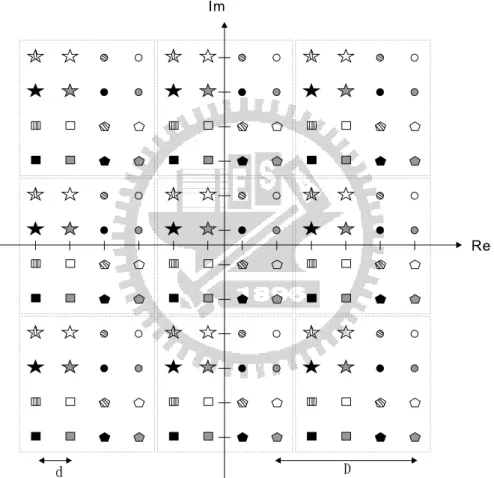
The expanded 16 QAM constellation can be divided into three groups in Fig. 3.6. One is the original 16 QAM constellation in the middle. In part A both real and imaginary parts can be added or subtracted a constant D. Only one dimension is changed in part B. The signal power in part B is given by:

εs−B = 4 16[ 4 X k=1 (Rk+ D)2+ 4 X k=1 Ik2] (3.17) = 4 16[ 4 X k=1 (Rk2+ 2RkD + D2) + 4 X k=1 Ik2] (3.18) = 4 16[ 4 X k=1 (Rk2+ Ik2) + 4D2+ 2(R1D + R2D + R3D + R4D)](3.19) = 4 16[ 4 X k=1 (Rk2+ Ik2)] + D2 (3.20) = εs+ D2. (3.21)

(23)

Re Im

d

D

Part A Part A

Part A Part B Part A

Part B

Part B Part B

Figure 3.6: The expanded 16 QAM constellation can be divided into three groups, original 16 QAM, part A, and part B.

The signal power in part A is given by:

εs−A = ₁₆4[ P₄ k=1(Rk+ D)2+ P₄ k=1(Ik+ D)2] = 4 16[ P₄ k=1(Rk2+ Ik2) + 8D2+ 2(R1D + R2D + R3D + R4D) + 2(I1D + I2D + I3D + I4D)] = 4 16[ P₄ k=1(Rk2+ Ik2)] + 2D2 = εs+ 2D2. (3.22)

(24)

is εs−new becomes εs−new = 1 9εs+ 4 9εs−B + 4 9εs−A (3.23) = 1 9εs+ 4 9(εs+ D 2_{) +} 4 9(εs+ 2D 2₎ _(3.24) = εs+ 4 3D 2_. _(3.25)

Because only one subchannel is modified a at time, the signal power of every subchannel becomes εs0 = 63 64εs+ 1 64εs−new (3.26) = εs+ D2 48. (3.27)

(25)

Chapter 4 The Subchannel Peak Reduction

Method

In this chapter, we present a subchannel based PAPR reduction method that we called Subchannel Peak Reduction method. We choose a few subchannels, called peak reduction (PR) subchannels. The symbols of the PR subchannels are transmitting at a slightly lower rate so that PAPR is reduced. In particular, the symbols transmitted on the PR subchannels may be individually rotated by multiples of 180◦ _{to minimize PAPR. Fig. 4.1 shows an example of bits-to-symbol}

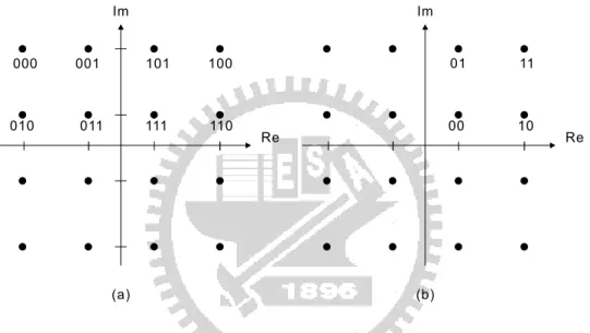
mapping for PR subchannels when the constellation is 16 QAM. The example given in Fig. 4.1(a) is for the case when the symbols on the PR subchannels may be rotated by multiples of 180◦ _{and Fig. 4.1(b) is for the case when the symbol}

can be rotated by multiples of 90◦_{. In the following discussions, we will consider}

the case of 180◦ _{rotation first. The method can be extended to the 90}◦_-rotation

case latter. In other words, the same input bits may be mapped to sk or −sk,

depending on which yields a smaller PAPR. If b-bit constellation are used for all subchannels, only (b − 1) bits can be transmitted on the PR subchannel. For non PR subchannels, bits are coded as symbol in the usual manner. Suppose the receiver output is ˆsk (before symbol detection). Then ˆsk and −ˆsk will be decoded

to the same bits. The transmitter does not need to send any side information. The receiver can make decisions of the transmitted symbols independently. The decoding errors of one subchannel does not affect other subchannels at all. The smallest PAPR using the SPR method can be found by exhausting all possible

(26)

combinations of rotations for the PR subchannel. We will show that when the subchannels are chosen properly, the optimal rotations of the PR subchannels can be computed efficiently. As the optimal solution is found by an exhaustive search (ES), we will call it SPR-ES. To further reduce the complexity, we propose an iterative approach (SPR-IT) to find suboptimal rotating for the PR subchannels. There is around 10 reduction in complexity. We will see that our method provides a tradeoff before PAPR reduction and complexity.

010 011 111 110 000 001 101 100 Re Im 00 10 01 11 Re Im (a) (b)

Figure 4.1: An example of bits-to-symbol mapping for PR subchannel when the constellation is 16 QAM. (a) The symbols on the PR subchannels may be rotated by multiples of 180◦_{. (b) The symbol can be rotated by multiples of 90}◦_.

4.1 An Exhaustive Search Scheme

Fig. 4.2 shows the block diagram of the SPR method. In the stage of initial bit-to-symbol mapping, the input bits are mapped to bit-to-symbols. For non PR subchannels, the bits are mapped to symbols in the usual manner. For PR subchannels (180◦

-rotation case), the bits are mapped to symbols in the first and second quadrants as demonstrated in the example show in Fig. 4.1(a). The output vector of bits-to-symbol mapping is s as indicated in Fig. 4.2. We can write it as the sum of

(27)

only PR subchannels,

s = s0+ s1. (4.1)

Suppose the PR subchannels are those with indices equal to multiples of J, then

s0 =                   0 s1 ... sJ−1 0 sJ+1 ... s2J−1 0 ...                   , s1 =                   s0 0 ... 0 sJ 0 ... 0 s2J ...                   .

These two vectors are respectively the output of 0_{non PR vector}0 _and 0_PR

sub-channel vector0 _{shown in Fig. 4.2.}

bits to symbol mapping non PR subchannel selector PR subchannel selector M-point IDFT s0 s0 s1 s b s0 1 x_ö

Figure 4.2: The block diagram of SPR method

We can generate all possible combinations of rotations of the PR subchannels. s0

1 = b . × s1, where b is an M × 1 vector with

[b]k =

½

1 or − 1, k=mJ

(28)

The notation .× denotes pointwise multiplication. The input vector of IDFT matrix is

s0 _{= s}

0+ s01. (4.3)

The output vector of the IDFT matrix is ¯x = w†_s0_{. For each possible rotation}

of the PR subchannels, we can compute the output vector and the PAPR of the output vector. We can then select the vector with the smallest PAPR.

We can also extend the method to the case of 90◦ _{rotations. In this case,}

the symbols of the PR subchannels may be rotated by multiples of 90◦_{. The}

bit-to-symbol mapping is like Fig. 4.1(b). Also the M × 1 rotation vector b can be written as

[b]k =

½

1 or − 1 or j or − j, k=mJ

0, otherwise. (4.4) The other process is the same. We defined n = 2 and n = 4 for multiplies of 180◦

and 90◦_.

In the following two examples, the IDFT size is 64 and 16 QAM with minimum distance d = 2 are used. A total 106_{random OFDM blocks are used in simulation.}

We consider three different numbers of PR subchannels P = 2, 4, and 8 for the low complexity purpose which will discuss in chapter 5. We choose n = 2.

Example 4.1. We selected the 0-th and 31−th subchannel. For P = 4, the PR subchannels are 0-th, 15−th, 31-th, and 47-th subchannel. The 8 PR sub-channels are 0-th, 7-th, 15-th, 23-th, 31-th, 39-th, 47-th, and 56-th subchannel. Fig. 4.3 shows the CCDF of PAPR for the case 180◦ _{rotation is used (n=2). The}

definition of CCDF for PAPR is as given in (2.5). For a CCDF of 10−4_{, We can}

see the 2 PR subchannels curve reduces about 0.5dB compares with the original OFDM transmitter and the PAPR reduction are almost 1dB and 2dB for 4 PR subchannels and 8 PR subchannels curves respectively.

(29)

4 6 8 10 12 10−4 10−3 10−2 10−1 100 PAPR0(dB) Pr(PAPR>PAPR0) SPR−ES, n=2 original 2 PRs 4 PRs 8 PRs

Figure 4.3: Example 4.1. SPR-ES: 2, 4, 8 PR subchannels and rotation factors are selected from {+1, −1}.

Example 4.2. In this example, we select the rotation factors from {+1, −1, +j,

−j}. The numbers of PR subchannels of ES are 2 and 4 and the corresponding

se-lected PR subchannels are {0, 31} and {0, 15, 31, 47}. From Fig. 4.4, when CCDF is 10−4_{, the 2 PR subchannels curve reduces about 0.7dB. The performance of 4}

(30)

4 6 8 10 12 10−4 10−3 10−2 10−1 100 PAPR0(dB) Pr(PAPR>PAPR0) SPR−ES, n=4 original 2 PRs 4 PRs

Figure 4.4: Example 4.2. SPR-ES: 2, 4 PR subchannels and rotation factors are selected from {+1, −1, +j, −j}.

(31)

4.2 An Iterative Approach Method

In the exhaustive method, we exhaust all possible combinations of rotations on the PR subchannels and choose the one that results in the smallest PAPR. Here we find the rotations for the PR subchannels in an iterative manner, one subchannel at a time. bits to symbol mapping non PR subchannel selector PR subchannel selector M-point IDFT s0 s₀ s1 s b rotation generator compute PAPR s0 1 x0

Figure 4.5: The block diagram of Iterative Approach method.

The block diagram is shown in Fig. 4.5. The input bits are mapped to symbols in the initial mapping as in the exhaustive method. Then we compute the IDFT output x = W†s and the corresponding PAPR. We find the peak on the IDFT output vector x. Say the peak occurs at n0 and |xn0| = maxi|xi|. Suppose now

we would like to see if the rotation of a PR subchannel, say i0, can reduce the

peak. We split the subchannels into s0 and s1. The vector s1 is non zero only in

the i0th entry, s1 = [0 · · · 0si00 · · · 0]T. When the i0-th subchannel is rotated by

180◦_{, we have s}0

1 = −s1. The new IDFT output x0 can also be written as

x0 _{= W}†_(s

0+ s01) (4.5)

= W†(s0+ s1− 2s1) (4.6)

= W†_{s − 2W}†_s

1 (4.7)

(32)

si0, so we have

x0 _{= x − 2w}∗

i0si0, (4.8)

where w∗

i0 is the i0-th column of the DFT matrix and ’∗’ denotes conjugate. (4.8)

means that x0 _{can be obtained by computing 2w}∗

i0si0 and subtracting it from x.

The computation of 2w∗

i0si0 requires only M multiplications and no addition.

We compute only the samples corresponding to the peak and find the new peak for x0_{. If it is smaller than the peak of x}

n0 then the i0th subchannel is rotated

by 180◦_{. Otherwise, it is not rotated. In a similar manner, we can determine one}

by one the transmitted symbols on the PR subchannels. As the rotations on the PR subchannels are not determind simultaneously, the solution is the suboptimal one.

In the following two examples, the IDFT size is 64 and modulation symbols are 16 QAM with minimum distance d = 2. Total 106 _{random OFDM blocks are}

used.

Example 4.3. IT method is used. The number of PR subchannels are 2, 4, and 8 and the subchannels are chosen as : {0, 31}, {0, 15, 31, 47}, and

{0, 7, 15, 23, 31, 39, 47, 56}. Fig. 4.6 show that case the symbols on SPR

subchan-nels are possible rotated by 180◦ _{(n = 2). We can see that there is more reduction}

(33)

4 6 8 10 12 10−4 10−3 10−2 10−1 100 PAPR0(dB) Pr(PAPR>PAPR0) SPR−IT, n=2 original 2PRs 4PRs 8PRs

Figure 4.6: Example 4.3. SPR-IT: 2, 4, 8 PR subchannels and rotation factors are selected from {+1, −1}.

(34)

Example 4.4. Fig. 4.7 show that case of SPR-IT, the rotation factors set is

{+1, −1, +j, −j} and the PR subchannel selections: {0, 31} for 2 PR subchannels, {0, 15, 31, 47} for 4 PR subchannels, are the same as Fig. 4.4 for SPR-ES method.

The two curves reduce at least 0.7 dB and 1.2dB of a CCDF 10−4 _{respectively.}

From Fig. 4.3 and Fig. 4.7, we find that when fixed the same set of rotation factors, the more PR subchannels we select and the more PAPR reduction at the same value of CCDF. 4 6 8 10 12 10−4 10−3 10−2 10−1 100 PAPR0(dB) Pr(PAPR>PAPR0) SPR−IT, n=4 original 2PRs 4PRs

Figure 4.7: Example 4.4. SPR-IT: 2, 4 PR subchannels and rotation factors are selected from {+1, −1, +j, −j}.

(35)

Example 4.5. In Fig. 4.8, we put two methods together with the same number of PR subchannels, which are {0, 7, 15, 23, 31, 39, 47, 56} and the same rotation factors set: {+1, −1}. As we mentioned in Chapter 2, for a given PAPR0,

the smaller the probability exceeds the PAPR0 is, the better the performance is.

We can see that exhaustive has better performance than iterative, especially when the PAPR thresholds are small. When the PAPR threshold PAPR0 is 6dB,

the probability exceeds PAPR0 are 0.3 and 0.1 for SPR-IT and SPR-ES method

respectively. 4 6 8 10 12 10−4 10−3 10−2 10−1 100 PAPR0(dB) Pr(PAPR>PAPR0) 8PRs, n=2 original SPR−ES SPR−IT

Figure 4.8: Example 4.5. SPR-ES v.s SPR-IT. 8 PR subchannels and rotation factors selected are from {+1, −1}.

(36)

Chapter 5 Computational Complexity

In this chapter, we consider the complexity of the SPR method proposed in chapter 4. We will also compare it with the tone injection method in chapter 3.

5.1 Exhaustive Search

The block diagram for the SPR method show in Fig. 4.2 can be drawn as Fig. 5.1. In Fig. 5.1, the IDFT block was put in front of the adder. We note that most of the elements only multiplies of J. As the result, the M-point IDFT after s0₁ in Fig. 5.1(a) can be replaced by a P -point IDFT. In Fig. 5.1(b), when P is defined as the number of PR subchannels. This can be done by using the lemma.

(37)

bits to symbol mapping non PR subchannel selector PR subchannel selector M-point IDFT s0 s1 s b s0 1 x_ö M-point IDFT bits to symbol mapping non PR subchannel selector PR subchannel selector M-point IDFT s0 s1 s b s0 1 x_ö M-point IDFT bits to symbol mapping non PR subchannel selector PR subchannel selector M-point IDFT s0 s1 s b s0 1 x_ö P-point IDFT bits to symbol mapping non PR subchannel selector PR subchannel selector M-point IDFT s0 s1 s b s0 1 x_ö (a) (b)

Figure 5.1: SPR-ES. (a) The IDFT block can put in front of the adder. (b) The M-point IDFT can be replaced by the P-point IDFT.

Lemma 1 Let W†_M be the M-point IDFT matrix. Assume M = J × P for some integers J and P . Define a P × 1 vector z0 _{= [z}

0, zJ, · · · , z(P −1)J]T. Define a M × 1 vector z, where [z]k= ½ zk, k=mJ, m = 0, 1, · · · , P − 1 0, otherwise. (5.1) Then we have

(38)

W†_Mz = √1 J      W†_P W†_P ... W†_P     z 0_.

Proof: Let a = W†_Mz, 0 ≤ n ≤ M − 1, then

an = 1 √ M M −1_X k=1 zkej2πkn/M (5.2) = √1 M(z0e j2πn0/M _{+ z} Jej2πnJ/M+ · · · + z(P −1)Jej2πn(P −1)J/M). (5.3) Let g = _√1 JW † Pz0, 0 ≤ n ≤ P − 1, then gn = 1 √ J 1 √ P P −1_X k=1 zkej2πkn/P (5.4) = √1 J 1 √ P(z0e j2πn0/P _{+ z} Jej2πn1/P + · · · + z(P −1)Jej2πn(P −1)/P). (5.5)

Firstly, we proof that the first P elements of a are equal to g, i.e., al = gl for

0 ≤ l ≤ P − 1. The l-th element of a is given by

al = 1 √ M(z0e j2πl0/M _{+ z} Jej2πlJ/M + · · · + z(P −1)Jej2πl(P −1)J/M) (5.6) = √1 J 1 √ P(z0e j2πl0/P _{+ z} Jej2πl/P + · · · + z(P −1)Jej2πl(P −1)/P) (5.7) = gl, f or 0 ≤ l ≤ P − 1. (5.8)

Secondly, we will show the following elements of a will repeat a0 to aP −1, i.e.,

(39)

given by al+q·P = √1_M(z0ej2π(l+q·P )0/M + zJej2π(l+q·P )J/M + · · · + z(P −1)Jej2π(l+q·P )(P −1)J/M) = _√1 M(z0e j2πl0/M_ej2πq·P 0/M _{+ z} Jej2πlJ/Mej2πq·P J/M+ · · · + z(P −1)Jej2πl(P −1)J/Mej2πq·P (P −1)J/M) = _√1 M(z0e j2πl0/M _{+ z} Jej2πlJ/M + · · · + z(P −1)Jej2πl(P −1)J/M) = al (5.9)

We can see the first P elements of a are equal to g and the next every P elements of a repeated the first P elements of a. 444

From the proof we can see that the elements of W†_Mz can be viewed as the elements of _√1

JW †

Pz0 repeating J times.

The output vector ¯x can be written as ¯ x = W†s0 (5.10) = W†_(s 0+ s 0 1) (5.11) = W†s0+ W†s 0 1 (5.12) = W†_s 0+ W†(b . × s1) (5.13) = x − W†_s 1+ W†(b . × s1). (5.14)

Let us look into the last term of (5.13). When a rotation vector bi = ubk,

where i, k ∈ {0, 1, · · · , nP _{− 1}, and u ∈ {−1, +j, −j}, then}

W†_(b

i. × s1) = W†(ubk. × s1) (5.15)

= uW†(bk. × s1). (5.16)

Because multiplying u does not need any complex multiplication and complex addition, the complexity will not increase. For n = 2, by using (5.16) to get the values of −W†(bi.×s1) and W†(bi.×s1) we only need to calculate W†(bi.×s1).

(40)

can be replaced by a P -point IDFT. There are nP _{possible b}

i. In conclusion,

we only need nP

n P -point IDFTs instead of nP P -point IDFTs to compute the

optimal rotations for the smallest PAPR. For a IDFT matrix size M which is the power of 2, we can apply a fast algorithm-Inverse Fast Fourier Transform (IFFT). The number of complex multiplications and complex additions required for an

M-point IFFT are 1

2M log2M and M log2M.

5.2 Iterative Approach

The iterative approach requires less complexity than the exhaustive method. Let us first consider one iteration. Recall from (4.5) when the i0-th subchannel is

rotated , the computation of the new DFT x0 is x0 = W†_s0

= W†_(s

0+ s

0

1) (5.17)

The vector s0₁ = rs1 and s1 = [0 · · · 0si00 · · · 0]

T_{, where r is the rotation factor}

and i0 is the underlying PR subchannel. When 180◦ rotation used r = −1, when

90◦ _{is used, r = −1, ±j. We note that the term x}0

1 = W†s 0 1 can be written as x0 = rW†_{s = rs} i0w ∗

i0, where wi0 is the i0-th column of DFT matrix and 0_∗0

denotes conjugate. The computation of x0 needs only complex multiplications, but it does not need IDFT.

For the 180◦_{-rotaion case (n = 2), when the i}

0-th subchannel is rotated by

180◦_{, the output vector x}0

= x − 2si0w∗i0. To compute x

0

, we need M complex multiplications and M complex additions. If we have P PR subchannels, the total complexity is P M complex multiplications and additions.

For the 90◦_{-rotation case (n = 4), r = −1, ±j. The output x}0

can be written as x0 = W†_s 0+ W†s 0 1 (5.18) = W†s0+ W†(ris 0 1) (5.19) = x − W†_s 1+ rsi0w ∗ i0. (5.20)

(41)

If ri = −1, we need M complex multiplications and additions. For ri = j or

−j, no complex multiplication is needed but 3M complex additions are needed

for computing x − si0w∗i0, +jsi0w∗i0, and −jsi0w∗i0. A total of MP complex

multiplications and 4MP complex additions are needed for P PR subchannels in SPR-IT method.

If the PR subchannel is selected properly, computing si0w ∗

i0 does not need

any complex multiplication. For example, when M = 64, the 0-th subchannel is selected to be the PR subchannel.

s0w0∗ = s0      1 1 ... 1     . (5.22) No complex multiplication is needed to compute (5.22).

5.3 Tone Injection (for passband

communica-tion)

Tone injection proposed by J. Tellado [6] is in the consideration of real multi-carrier. We modified it to passband communication in section 3.2 and in this section we will calculate the complexity. We will divided s into two vectors like SPR method. One is a M × 1 vector s1 contained one subchannel which is going

to be modified, the other is a M × 1 vector s0 = s − s1. Suppose the k-th

sub-channel is going to change. We can write down s1 which has only one value on

the k-th subchannel, s1 =            0 ... 0 sk 0 ... 0            .

(42)

Subtract s by s1 then we get a vector s0, s0 =              s0 s1 ... sk−1 0 sk+1 ... sM −1              .

After modification which was discussed in section 3.2, s1 becomes ¯s1:

¯s1 =            0 ... 0 sk 0 ... 0            + pkD            0 ... 0 1 0 ... 0            + jqkD            0 ... 0 1 0 ... 0            (5.23) = s1+ (pkD + jqkD)ek, (5.24)

where ek= [0, · · · , 0, 1, 0, · · · , 0]T. Let m = pkD + jqkD. After IDFT matrix, we

get

¯

x = W†(s0+ ¯s1) (5.25)

= W†_s

0+ W†¯s1 (5.26)

(5.26) can also be written as ¯ x = x − W†_s 1+ W†¯s1 (5.27) = x − W†_s 1+ W†(s1+ mek) (5.28) = x + mW†ek. (5.29)

W†ek is equal to 1 · w∗k and it does not need any IDFT matrix. For the k-th

(43)

(i) When m = 0, ¯x = x. The M-point IDFT is not included in complexity calculation.

(ii) When m = D or m = jD or m = −jD or m = −D. We need M complex multiplications for m = D to multiply w∗

k. 4M complex additions are also needed

because here we have 4 values of m and each m needs M complex additions in (5.29).

(iii) The remainders: m = D + jD, m = D − jD, m = −D + jD, and

m = −D − jD. When m = D + jD,

mW†ek = (D + jD)W†ek (5.30)

= DW†ek+ jDW†ek. (5.31)

Both DW†ek and jDW†ek are calculated in (ii). Therefore, we do not need any

complex multiplication but M complex additions to add DW†ek and jDW†ek

together. 4M complex additions are the same purpose as in (ii). Then in this part we use only 5M complex additions and no complex multiplication.

Put three groups together then we realize that to change a subchannel use tone injection method needs M complex multiplications and 9M complex additions. For total M subchannels, the complexity becomes M ×M complex multiplications and 9M × M complex additions. When M gets larger, the complexity increase faster.

We put three methods comparison together in the following table.

Table 5.1: Complexity Comparison of the SPR-ES, SPR-IT, and Tone Injection methods. If P ∈ {0,M

4 −1,M2 −1,3M4 −1} , the complex multiplication of SPR-IT

(n=2) and SPR-IT (n=4) are zero.

complex multiplications complex additions SPR-ES 1

2(nP −1)P log2P (nP −1)P log2P + MnP

SPR-IT (n = 2) P M P M

SPR-IT (n = 4) P M 4P M Tone Injection [6] M2 _9M2

(44)

Example 5.1 Both SPR-ES and SPR-IT select 8 PR subchannels:

{0, 7, 15, 23, 31, 39, 47, 56} and the rotation factors are selected from {+1, −1}.

The IDFT size is 64. a = 1, D = 8 in Tone Injection method. The complexity comparison of the three methods are put in Table. 5.2

Table 5.2: Example 5.1. Complexity comparison of the SPR-ES, SPR-IT, and tone injection methods. 8 PR subchannels are selected for ES and SPR-IT and the rotation factors are selected from {+1, −1}. a = 1, D = 8 in tone injection method.

complex multiplications complex additions SPR-ES 1536 19456

SPR-IT 256 1024 Tone Injection [6] 4096 36864

(45)

Chapter 6 Simulation Results

In this chapter we will see more simulation results. The block diagram of the OFDM system using SPR method is shown in Fig. 6.1. The IDFT block at the transmitter is put in the SPR method block in Fig. 4.2 and Fig. 4.5. The input symbols have the same variance εs because there is usually no bit/power

allocation in the OFDM system. The symbols are assumed to be zero mean and uncorrelated, which is usually a reasonable assumption after proper interleaving of the input bit stream. The autocorrelation matrix of the input vector s is thus Rs = εsIM, where IM is a M × M identity matrix. Then the output vector of

IDFT matrix x = W†s has autocorrelation matrix Rx = E[xx†] given by:

Rx = W†RsW = εsIM. (6.1)

Therefore x are uncorrelated and their variances are the same, equal to εs.

Fig. 6.2 shows the clipping with a maximum permissible amplitude A. The operation of clipping a real number x can be written as:

y = f (x) =

½

x, |x| ≤ A

(46)

16QAM SPR P/S CP clipping channel remove CP S/P DFT demod noise bit stream s x y

Figure 6.1: The OFDM system with SPR method.

- A A

Figure 6.2: A clipping with maximum amplitude A.

In Fig. 6.1, there is a clipping block before the channel. The n-th element of the transmitted signal y can be written as

yn = yr,n+ jyi,n, (6.3)

where yr,n and yi,n are the real and imaginary part of yn respectively. The

am-plitude clipping operates on yr,n and yi,n individually. The output of clipper

becomes f (yr,n) + jf (yi,n). The clipping ratio γ is defined as

γ = A√max P0 , (6.4) where Amax = √ A2 _{+ A}2 ₌√_2A.

(47)

constellation points become smaller after modulo-D process and hence the bit error rate (BER) may be increased slightly.

The BER depends on the signal power and the noise power. The BER curves are plotted against the signal-to-noise (SNR). But here we will plot the BER curves of average-transmission-power-to-noise ratio (P0/N0), where P0 is the

av-erage transmission power of y before clipping and N0 be the noise variance of

AWGN channel.

We will see some examples in the following. In our simulations, the IDFT size is 64 and total 105 _{random OFDM blocks are used in the simulation. The}

input symbols are 16 QAM. P0 is the same as εs. The SPR method uses 8 PR

subchannels: {0, 7, 15, 23, 31, 39, 47, 56} and the rotation factors are selected from

{+1, −1}. a = 1 in the tone injection method. We selected 8 PR subchannels

and SPR-ES will lose 8 bits for a block transmission.

Fixed noise variance (N0 = 1). The noise variance N0 is fixed to 1. The

BER of SPR-ES and tone injection are in Fig. 6.3. We can see under the same noise variance, SPR-ES has better BER performance. When BER is fixed to 10−3_{, P}

0 are 16.5 dB and 17.3 dB for SPR-ES and tone injection. This is meant

that the average transmission power are 44.67 and 53.7 respectively. The average transmission power of SPR-ES is 20% smaller than tone injection. However, SPR-ES used 8 PR subchannels and lost 8 bits when 16 QAM constellation is used. This is equivalent to a loss of 3% in transmission rate. Under the same noise variance and BER, SPR-ES needs smaller average transmission power than tone injection. The CCDF of PAPR of both methods are in Fig. 6.4. For large PAPR0 SPR-ES has better performance than tone injection.

(48)

5 10 15 20 10−3 10−2 10−1 100 P₀/N₀ (dB) Probability of error SPR−ES Tone Injection [6]

Figure 6.3: BER. N0=1. SPR-ES uses 8 PR subchannels and rotation factors are

selected from {+1, −1} and tone injection.

4 6 8 10 12 10−3 10−2 10−1 100 PAPR0 (dB) Pr(PAPR > PAPR0) SPR−ES Tone Injection [6]

Figure 6.4: PAPR. N0=1, BER=10−3. SPR-ES uses 8 PR subchannels and

(49)

Fixed average transmission power. (P0 = 10). In this example, we

fixed the average transmission power P0 to 10. When fixed P0, the minimum

distance of the constellation used the tone injection method is smaller than that of SPR-ES. The minimum distance of SPR-ES and tone injection are 2 and 1.88 respectively. We can see SPR-ES has better BER performance in Fig. 6.5. For a BER of 10−3_{, SPR-ES is 1 dB less than tone injection.}

5 10 15 20 10−3 10−2 10−1 100 P 0/N0 (dB) Probability of error SPR−ES Tone Injection [6]

Figure 6.5: BER. Fixed average transmission power. P0 = 10. SPR-ES

uses 8 PR subchannels and rotation factors are selected from {+1, −1} and tone injection.

(50)

Fixed average transmission power and the clipping ratio. (P0 = 10,

γ = 2). In the following two examples we add a clipping operator before the signal

passing through the channel. The BER performance after adding the clipping is worse, especially for the smaller clipping ratio γ. If P0 and γ are fixed, the peak

value can be decided. When γ = 2 and P0 = 10 we can get Amax = 6.32 and

the corresponding A = 4.47. The peak value of the two methods are all equal to (4.47)2 _{+ (4.47)}2 _{= 39.96. Under the same peak value and P}

0, SPR-ES has

slightly better BER performance.

Figure 6.6: BER. Fixed average transmission power and the clipping ratio. (P0 = 10, γ = 2). SPR-ES uses 8 PR subchannels and rotation factors

(51)

Fixed average transmission power and the clipping ratio. (P0 =

10, γ = 3). In this example, γ = 3 and P0 = 10. Amax = 9.49 and the

corresponding A = 6.71. The peak value of the two methods are all equal to (6.71)2 _{+ (6.71)}2 _{= 90.05. SPR-ES in this example still has better performance}

than the tone injection method.

Figure 6.7: BER. Fixed average transmission power and the clipping ratio. (P0 = 10, γ = 3). SPR-ES uses 8 PR subchannels and rotation factors

(52)

Chapter 7 Conclusion

In this thesis, we proposed a new method called SPR. SPR method reduces PAPR by multiplying rotations to the symbols of the PR subchannels individu-ally. Two schemes of SPR method were introduced. Simulation results showed both shcemes can reduce at least half dB from the original system with no PAPR reduction method when only two PR subchannels were selected. The average transmission power of SPR method remains the same. A few bits were lost on the PR subchannels but no side information is needed. Although the computa-tional complexity increases, the numbers of complex multiplications and complex additions are few compared with tone injection method.

(53)

Bibliography

[1] J. A. C. Bingham, “Multicarrier Modulation For Data Transmission: An Idea Whose Time Has Come,” IEEE Commun. Mag, vol. 28, no. 5, May 1990, pp. 5-14.

[2] M. Aldinger, “Multicarrier COFDM scheme in high bit rate ratio local area network,” in Proc. 5th IEEE Int. Symp. Personal, Indoor and Mobile Radio

Communications, The Haugue, The Netherlands, Sept. 1994, pp. 969-973.

[3] ETSI, “Digital Video Broadcasting; Framing, Structure, Channel Coding and Modulation for Digital Terrestrial Television (DVB-T),” ETS 300 744, 1997.

[4] ETSI, “Digital Audio Broadcasting (DAB) to Mobile, Protable and Fixed Receivers,” ETS 300 401, 1994.

[5] A. Ruiz, John M. Cioffi, and S. kasturia, Discrete Multiple Tone Modulation with Coset Coding for The Spectrally Shaped Channel, IEEE Transcation on Communications, Vol. 40, No. 6, Page (s) : 1012-1029, June 1992. [6] J. Tellado, Multicarrier Modulation with Low PAR: Applications to DSL and

Wireless Kluwer Acdamic, Press. 2000.

[7] R. O’Nell and L. B. Lopes, “Envelope Variations and Spectral Splatter in Clipped Multicarrier Signals,” Proc. IEEE PIMRC ’95, Toronto, Canada, Sept. 1995, pp. 71-75.

(54)

[8] A. E. Jones, T. A. Wilkinson, and S. K. Barton,“Block Coding Scheme for Reduction of Peak to Mean Envelope Power Ratio of Multicarrier Transmis-sion Scheme,” Elect, Lett, vol. 30, no. 22, Dec. 1994, pp. 2098-99.

[9] J. A. Davis, and J. Jedweb,“Peak-to-Mean Power Control in OFDM, Go-lay Complementary Sequences, and Reed-Muller Codes” IEEE, Trans Info.

Theory, vol. 45, no. 7, Nov. 1999, pp. 2397-17.

[10] K. G. Paterson and V. Tarokh,“On the Existence and Construction of Good Codes with Low Peak-to-Average Power Ratios,” IEEE, Trans Info. Theory, vol. 45, no. 6, Sept. 2002, pp. 1974-87.

[11] R. W. B¨auml, R. F. H. Fisher, and J. B. Huber, Reducting the Peak-to-Average Power Ratio of Multicarrier Modulation by Selected Mapping ,”

Elect, Lett, vol. 32, no. 22, Oct. 1996, pp. 2056-57.

[12] P. Van Eelvelt, G. Wade, and M. Tomlinson, Peak to average power reduc-tion for OFDM schemes be selective scrambing.Elect, Lett,, vol. 32, no. 21, pp. 1963-1964, Oct. 1996.

[13] S. H. M¨uller and J. B. Huber, OFDM with Reduced Peak-to-Average Power

Ratio by Optimum Combination of Partial Transmit Sequences,Elect, Lett, vol. 33, no. 5, Feb. 1997, pp. 368-69.

[14] C.-L. Wang, M.-Y. Hsu, and Y. Ouyang, A low-complexity peak-to-average power ratio reduction technique for OFDM systems, in Proc. 2003 IEEE Global Telecommun. Conf. (GLOBECOM 2003), San Francisco, CA, Dec. 2003, pp. 2375-2379.

[15] C.-L. Wang and Y. Ouyang,Low-Complexity Selected Mapping Schemes for Peak-to-Average Power Ratio Reduction in OFDM Systems, IEEE Transca-tion on CommunicaTransca-tions, Vol. 53, no. 12, Dec. 2005.

(55)

[16] S. H. Han and J. H. Lee, PAPR Reduction of OFDM Signals Using a Reduced Complexity PTS Technique, IEEE Sig. Proc. Lett., vol. 11, no. 11, Nov. 2004, pp. 887V90.