A Pattern Growth Approach for Frequent Subgraph Mining

全文

(1)A Pattern Growth Approach for Frequent Subgraph Mining Chia-Hui Chang and Cheng-Tao Ho Department of Computer Science and Information Engineering, National Central University No. 300, Jhungda Road, Jhungli City, Taoyuan 320, Taiwan chia@csie.ncu.edu.tw, ctho@db.csie.ncu.edu.tw ABSTRACT Graph mining has wide applications in chemistry, biology and computer networks. This kind of structure pattern mining might encounter more duplication cases due to graph isomorphism. Pattern growth approach has been shown to perform well for unstructured pattern mining, such as itemset and sequential patterns. In this paper, we shall examine whether such approach can also works for structured pattern mining. We propose a graph mining algorithm which enumerates frequent patterns by combining known frequent patterns with local frequent edges discovered via embedding lists. The embedding list technique not only facilitates the discovery of local frequent edges but also averts subgraph isomorphism checking. The empirical study on synthetic and real datasets demonstrates that HybridGMiner outperforms the algorithm gSpan but seconds to Gaston.. pattern with local one, thus, avoiding the database scans for other generate-and-test approaches. As for the second issue, a common method is to adopt canonical form checking for graph isomorphism as proposed by gSpan [18]. In this paper, we propose an algorithm (namely HybridGMiner) that combines the pattern growth idea (i.e., local-frequent) with the canonical form for mining all frequent sub-graph patterns. Our empirical study on synthetic and real datasets shows that the HybridGMiner can achieve a substantial performance gain over the algorithm gSpan. The rest of this paper is organized as follows. Section 2 defines the graph pattern mining problem. Section 3 introduces related works. We discuss our algorithm and some tough problems in Section 4. Section 5 devotes to data generation and the experiments. Finally, this paper closes with an integral evaluation and the future works.. 1: Introductions. 2. Problem Definition. Over the past few years, a considerable number of studies have been conducted on frequent itemsets and sequential patterns. However, such patterns completely ignore link structures among data. In reality, there is a strong need for graph mining which retains the structure information among data. For example, in the drug design process, one of the key steps is to identify the chemical compounds that display the desired and reproducible behavior against the disease in a biological experiment [9][10]. In such scenarios, the atom and chemical bound of a chemical compound correspond respectively to the nodes and the edges of a graph structure. As another example, graph mining can also be used in software behavior graph for detecting program regions containing noncrashing bugs. In addition, graph mining can also be applied for efficient indexing [6], or enhancement of semi-structure database storage [5]. The goal of graph analysis is to find the common structure or the common relationship between the data, which can be used for further prediction and classification. Graph mining mainly will encounter two kernel problems, namely duplicated enumeration and subgraph isomorphism. The first issue is a common problem in pattern mining while the second is a new problem for structure pattern mining like tree patterns and graph pattern. Non-structure pattern mining has received great attention in the past ten years and we have a lot of literatures on frequent itemset mining [1] as well as sequential pattern mining. The pattern growth method proposed in [16] has demonstrated better performance over other approaches since it generates only frequent patterns by combing a known frequent. In this paper, we limit our problem on undirected labeled and connected simple graph. Definition 2.1: Labeled Graph A labeled graph G can be represented as a four tuple G = (V, E, L, l), where V is the set of vertices, E ⊆ V × V is a set of edges, L is a set of labels, and l is a labeling function V ∪ E → L, that produces labels from L to all edges and vertices. Definition 2.1: Connected Graph G = (V, E, L, l) is a connected graph if ∀ u, v ∈ V(G), there exits w1, …wn ∈ V(G), such that {(u, w1), (w1, w2), …(wn-1, wn), (w1, v)} ∈ E(G). Definition 2.3: Subgraph / Graph Isomorphism. Two graphs G and G’are isomorphic if there exists a bijective mapping f of vertices, f: V(G) → V(G’ ), such that u V (G ), lG (u ) l G ' ( f (u )), and (u , v) E (G ), ( f (u ), f (v)) E (G ' ) and l G (u , v) l G ' ( f (u ), f (v)). A graph G’has subgraph isomorphism with G if G is isomorphism to a subgraph of G’ . Definition 2.4: Support Given a graph database GDB = {Gi | i = 0, …, n}. The support of an arbitrary graph g in GDB is defined as follow: s ( g , GDB ) . ( g , G. G i GDB. i. ). 1 if G has subgraph isomorphism with g.  ( g , G)   0 Otherwise.  . As shown in Figure 1, the pattern (A-B) has five occurrences in GDB (as shown in thick lines) and support 3. Given a graph database GDB and a minimum. - 322 -.

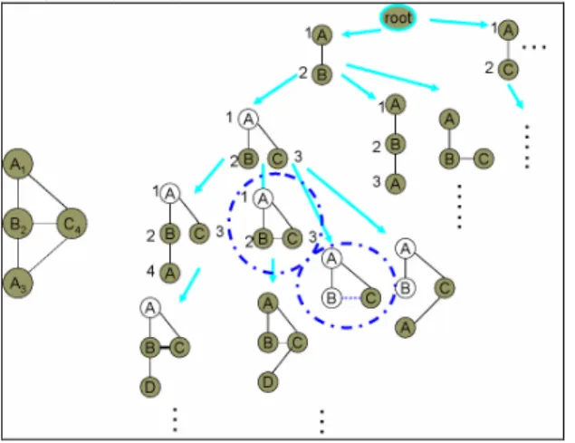
(2) support, minSup, Frequent Subgraph Mining is to find every subgraph g, such that s(g, GDB) ≧ minSup.. Figure1: Example database and pattern (A-B). So far, there have been several algorithms for mining graph pattern such as AGM [8], FSG [9], MoFa [3], gSpan [15], FFSM [6], and Gaston [12]. In the next section, we will compare the related works by analyzing their approach, and propose a hybrid method to improve mining efficiency.. 3. Related Work. Designing an algorithm to find frequent subgraphs in graph data sets is challenging and computationally intensive, as graph and subgraph isomorphisms play a key role throughout the computations. For this reason, earlier work has focused on approximation algorithms (e.g. SUBDUE [4]). In recent years, several algorithms have been developed capable of finding all frequently occurring subgraphs with reasonable computational efficiency. AGM [8] discovers frequent subgraphs using a breadth-first approach, and grows the frequent subgraphs one-vertex-at-a-time. It uses a canonical labeling scheme based on the adjacency matrix representation to distinguish subgraphs. To speedup subgraph isomorphism computation, it keeps track of previously found embeddings of a frequent pattern to improve the efficiency but at the expense of increased memory requirements. FSG [9] also adopts a breadth-first enumeration, but with a more efficient graph representation structure and edge-growth approach. gSpan [15] finds the frequently occurring subgraphs following a depth-first approach. GSpan has two approaches in pattern growth: from the right most path of the spanning tree or from one of the frequent edges. Every time a candidate subgraph is generated, its canonical label (called DFS code) is computed. If the computed label is the minimum one, the candidate is saved for further exploration of the depth search. If not, the candidate is discarded because there must be another path to the same candidate. gSpan does not keep the information about all previous embeddings of frequent subgraphs which saves the memory usage. According to the reported performance in [15], gSpan performs better than FSG on synthetic data sets. MoFa also finds frequent substructures using a depth-first approach, i.e., once a frequent subgraph has been identified, it then proceeds to explore all frequent subgraphs containing the frequent subgraph. To reduce the number of subgraph isomorphism operations, it keeps the embeddings of previously discovered subgraphs. However, their candidate subgraph generation scheme does not ensure that the same subgraph is generated only once (no canonical form is used). As a result, they end up generating and. determining the frequency of the same subgraph multiple times. Therefore, FFSM [6] adopts a graph canonical form and two efficient candidate proposing operations: FFSM-Join and FFSM-Extension, to improve the mining efficiency. Finally, Gaston [12] is the most efficient algorithm so far [10]. This algorithm divides the complex graph enumeration problem into three simpler subproblem of path, tree and cyclic graph. Therefore, it simplifies the complex canonical form checking for the path and tree patterns. Gaston also uses embedding list to avoid subgraph isomorphism problem. Note that FFSM and Gaston all use the mechanism of embedding lists to avoid subgraph isomorphism checking. However, one feature that has not been fully taken advantage of is the presence of local frequent patterns. Local frequent items have been explored in the context of sequential pattern mining to improve mining efficiency [13]. That is, instead of adding every global item to a frequent pattern, we only need to extend items that are known to be frequent in the sequences containing the pattern. Therefore, there is no need for subgraph isomorphism checking. In this paper, we should explore how extending from local frequent items can affect the mining efficiency.. 4. HybridGMiner Algorithm. Recall that two key points in graph mining are pattern enumeration and support counting. To avoid duplicate enumeration, one can either adopt postfiltering or self-pruning via canonical form checking. As for support counting, embedding lists have been used in various forms to speedup subgraph isomorphism checking. In the extreme case, subgraph isomorphism can be completely avoided as in this paper. Therefore, the embedding lists used in HybridGMiner record every occurrence of a subgraph pattern in each graph of the database. For this reason, we adopt canonical form (similar to gSpan [15]) checking to avoid duplicate enumeration since the memory requirement is already high for storing embedding lists. In a way, embedding lists is like the projected database of a frequent pattern in the context of pattern growth [5], however, the extension of an existing pattern is much complicated than sequential patterns where the extension direction is only forward. Thus, we should focus on the extension mechanism here.. 4.1 Pattern Growth. Pattern growth strategy enumerates pattern in a depth first manner. It starts with each frequent 1-edge, where the occurring positions of the edge in the graph database are recorded in an embedding list. From the embedding list, we check the database for extendable frequent 1-patterns, which are edges that are connected to nodes in the existing patterns. If an extendable edge is frequent, new pattern is formed and its embedding list is computed for further extension. The recursive process stops when there is no frequent extendable edge for a pattern. Note that we grow patterns edge-by-edge, which follows the anti-monotone spirit, i.e., if g1 is a subgraph of g2, the support of g2 is less than g1. Thus if. - 323 -.

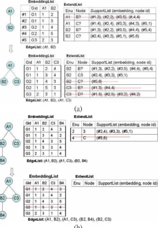
(3) g1 is not frequent, there is no need to grow pattern from g1. Figure 2 shows the extendable edges for some patterns based on the graph on the left. For pattern (A-B), the extendable edges are (A1,C4), (B2,A3) and (B2,C4). The subscripts denote the node id in order to distinguish nodes with the same labels. If (A,C) is a frequent edge, new pattern can be formed and its embedding list must be calculated. For this new pattern (A-B,A-C), we will have extendable edges (B2,A3), (B2,C4) and (C4,A3).. form C1 is smaller than C2, we can give up pattern G2 since it must be generated before. Note that we can also store all previous patterns and compare them with a new pattern to avoid such duplication; however, the cost will be more space and time.. Figure 3: Canonical Form. 4.2 Finding Extendable Edges. Figure 2: HybridGMiner enumeration process Similar to sequential pattern mining, edges are given orders to avoid duplication. For example, starting with pattern (A-B), we won’ t need to enumerate (A-A) since such patterns have been enumerated under pattern (A-A). The challenge of graph mining is that the number of extendable points is more than one. For sequential pattern, there is only one point, i.e. the rightmost way to grow a pattern; however, for graph patterns, any nodes in the existing pattern can be extended. Thus, an order must be assigned to determine which nodes to be extended first. One simple way is to give an enumeration order for nodes in the pattern. For example, the numbers beside the nodes on the right side of Figure 2 show the enumeration order of nodes. For 1-edge patterns, the enumeration order is based on the order of labels. When new nodes are added, they are given enumeration number accordingly. For example in pattern (A1-B2, A1-C3), the enumeration order is A, B, C. Thus, if all three extendable edges are all frequent, we will add edge (B,A) first, then (B,C), followed by (C,A). Graph mining is more complicated than sequential pattern mining for isomorphism problem, which can’ t be avoided by simple orders. However, it can be avoided via canonical form checking as in gSpan [18]. Figure 3 shows an example graph with two different enumeration orders. To avoid such duplication, each graph must be permutated (i.e. different enumeration order) to generate a canonical form for each permutation. If any permutation has canonical form smaller than the original enumeration order, then this pattern can be pruned. Thus, when enumerating graph pattern G2 (with canonical form C2) in Figure 3, we try to permute the pattern and get graph pattern G1. Since the canonical. The concept of local frequent edges is easy to understand, however, the calculation of extendable edges is much complicated in graph mining and depends greatly on the data structures we used for graphs and embedding lists. The good news is that the embedding lists for graph patterns, i.e. the projected database of a pattern in sequential pattern completely avoid the costly isomorphism checking. Before the enumeration, we scan the database once to find frequent edges. Then, any non-frequent edges in the graphs will be removed. For example, suppose we have minimum support 3, the graphs in Figure 1 will become those in Figure 4 after the preprocessing steps. Each embedding of a pattern is a mapping of the nodes between the pattern and some graph in the database as shown on the left of Figure 5 (a) and Figure 5 (b). For example, the pattern (A1-B2) has embedding list (G1,1,2), (G1,1,3), (G2,1,4), (G2,1,5), (G3,2,3), where the first component denotes the graph id and the rest components denotes the corresponding node numbers in the graph. As the pattern grows, new nodes are added to those embeddings supporting the pattern.. Figure 4: Removing nonfrequent edges in Figure 2 (minimum support=3). To find the extendable edges for a pattern, we should look into each embedding and find all edges with node numbers occurring in the embedding list. For example, for the first embedding (G1, 1, 3) of pattern (A1-B2), we can add node B3 and C4 from the first node A1, and node B3 from the second node B2. As another example, we can add for embedding (G3,2,3) node C1 from the first node (A2) and B4 and C6 from the second node (B3). We use a list of 2-tuple (#embedding, node id) to represent the support from an embedding with new added node (ExtendList) as shown on the right of Figure 5 (a) and Figure 5 (b). For example, node B from the. - 324 -.

(4) first node will be supported by embeddings #1, #2, #3 and #4 with new node 3, 2, 5, and 4, respectively. Since the first two embeddings belong to graph-01 and the last two embeddings belong to graph-02, the support count is two. As another example, node C from the first node is supported by all five embeddings with new node, 4, 4, 3, 3, and 1, respectively. As shown on top of Figure 6(a), pattern (A,B) has three frequent extendable edges: one (C) from the first node, two (B and C) from the second node.. is an existing node (C3) and one that C is a new node (C?).. 4.3 Pseudo Code. Figure 6 shows the pseudo code of the HybridGMiner algorithm. Step 1 scans the database once to find frequent 1-edge and remove nonfrequent edges at the next scan (step 2). Beginning with each frequent 1-edge e=(A1, A2) as the core pattern, we check for extendable edges from the nodes A1 and A2 of each embedding, i.e. constructing ExtendList (step 4). Then, it calls procedure Subgraph_Mining to enumerate other frequent patterns beginning with edge e. Step 6 deletes the edge e from database to narrow the size of database. Input: A graph database GD and minimum support minsup; Procedure HypbridGMiner() 1: Scan database GD once to find frequent edges, S1; 2: Remove non-frequent edges in GD; 3. for each edge e=(A1,A2) in S1 do // sorted by A1, A2 4: Initialize pattern p from e; // Construct p.ExtendList; 5: Output pattern p; Subgraph_Mining(p); 6: Remove edge e in GD; 7: if (|GD|<minsup) break; 8: end for. (a). Procedure Subgraph_Mining(Pattern p) 9: Remove nonfrequent edges in p.ExtendLists; 10: for each entry e=(Enu,Node,List) in p.ExtendList do // sorted by Enu, Node 11: EdgeListp.EdgeList{(Enu, Node)}; 12: if (!canonical(EdgeList)) then break; 13: Initialize a new pattern pnt from p; 14: pnt.EdgeListEdgeList; 15: pnt.ExtendList =p.ExtendList -{e}; 16: pnt.Refinement(Node, List); 17: Output pattern p; Subgraph_Mining(pnt); 18: endfor Method Pattern.Refinement(N, SupportList) 19: Remove any embeddingList entry that is not in SupportList; 20: if (N is not a new node) then return; 21: EnuNo++; // an index for the number of nodes in the pattern; 22: for each occurrence (Em#, Nid) in SupportList do; 23: AddNode(Em#, Nid); // insert new node to Em# 24: Gid= GetGid(Em#); // Get Gid of Em# 25: for each connected node Qid from node Nid in GD[Gid] do 26: if (Qid Nodesof(Em#)) then 27: Add (Em#, Qid) to ExtendList at entry (EnuNo, Qid.label).SupportList; 28: endfor 29: endfor 30: for each edge e=(Enu, Node, List) in ExtendLists do 31: for each occurrence (Em#,Nid) in List do 32: if (Nid= GetNode(Em#,Enu)) then 33: Remove (Em#, Nid) from ExtendList at entry (Enu, Node).SupportList; 34: Add (Em#, Nid) to ExtendList at entry (Enu, EnuNo).SupportList; 35: endif 36: endfor 37: endfor. (b) Figure 5: Refinement of embedding lists Since patterns grow from small enumerated node to large ones, the order will produce a spectacular result: the next pattern’ s ExtendList can be inherited from the old pattern’ s ExtendList by adding edges to the last extensible node and small refinement of the inherited ExtendList. Such an inheritance policy will increase the speed of mining, but slightly increase memory usage. Figure 5 (a) shows the inheritance of ExtendList of pattern (A-B, A-C) from that of pattern (A-B) and the refinement of ExtendList. Only new node C has to be examined to find extendable nodes. Note that only nodes that are not in the mapping table can be added. For example, two possible edges are (C, B) and (C, D) from the newly added node (C3). However, both of them are not frequent, thus, can be removed. For nodes that are in the mapping table, we need to refine the ExtendList since some of the nodes may be inserted as a new node. For example, when node C is added to the first node, i.e. edge (A1, C3), node 4, 3, and 1 of graph G1, G2 and G3, respectively are added as the new node of the pattern. Thus, the extend list for node C from the second node must be separated to two cases: one that C. Figure 6：HybridGMiner Algorithm For each frequent extendable edge e in the ExtendList (step 10), we create a new pattern by adding e to the existing pattern p (step 11), if the new pattern is not a canonical form, we simply skip to the next extendable edge (step 12). Otherwise, a new pattern pnt is constructed by copying from pattern p (step 13), then. - 325 -.

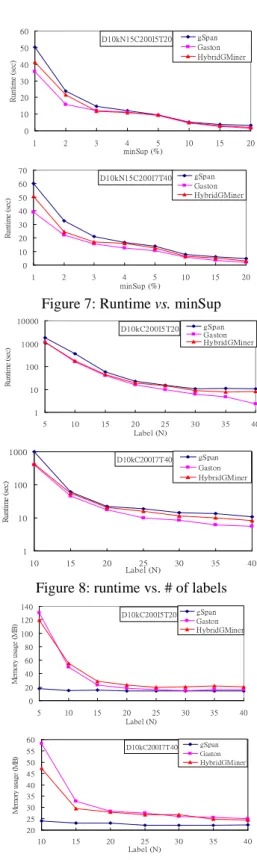
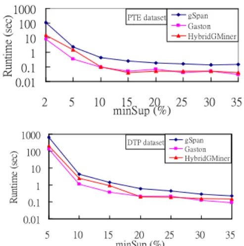
(5) updating EdgeList, ExtendList and mapTable (step 14-16). Pattern refinement deals with the update of ExtendList and EmbeddingList. First, it removes embeddings that are not in the supportList from EmbeddingList (step 19). If a new node is added, we must insert the new node into each embedding of the mapTable (Line 22-23), then check for extendable nodes from the new node in the corresponding graph (step 25-28). Finally, if the inserted new node has been referenced in other extendable edges, we should update those entries in ExtendList respectively (step 30-37).. 60. gSpan Gaston HybridGMiner. D10kN15C200I5T20. Runtime (sec). 50 40 30 20 10 0 1. 2. 3. 70. 10. 50. Runtime (sec). 15. 20. gSpan Gaston HybridGMiner. D10kN15C200I7T40. 60. 5. Experiments. 4 5 minSup (%). 40 30 20 10. We tested our algorithm on both synthetic data and real world data. Synthetic data are generated by data generator proposed by Kuramochi and Karypis with parameters used in [12][15]. The real world data includes two sets related to the chemical compound dataset. Experiments were done on CPU Intel Pentium 4 2.8 GHZ machines with 1.5 GB main memory, running the Linux Fedora core 4.. 0 1. 2. 3. 4 5 minSup (%). 10. 15. 20. Figure 7: Runtime vs. minSup 10000. gSpan Gaston HybridGMiner. D10kC200I5T20 Runtime (sec). 1000 100 10. 5.1 Synthetic Data. 1 5. 10. 15. Runtime (sec). 1000. 20 25 Label (N). 30. 35. 40. gSpan Gaston HybridGMiner. D10kC200I7T40. 100. 10. 1 10. 15. 20. 25 Label (N). 30. 35. 40. Figure 8: runtime vs. # of labels 140 Memory usage (MB). gSpan Gaston HybridGMiner. D10kC200I5T20. 120 100 80 60 40 20 0 5. 10. 15. 20 25 Label (N). 30. 60 D10kC200I7T40. 55 Memory usage (MB). We implement a similar data generator as proposed by Kuramochi et al. in [12]. However, the edges are generated without labels, increasing the probability of graph isomorphism. The meanings of parameter and default value are shown in Table 1. We have two default settings: one has seed average length of 5 (i.e., |I| = 5) and average graph size of was 20 (|T| = 20), the other has seed average length of 7 (|I| = 7) and average graph size of 40 (|T| = 40). Parameter Description Default D The number of graph in dataset. 10K N The number of different label. 15 C The number of seed. 200 I The average length of a seed. 5 7 T The average length of a graph. 20 40 Table 1: The parameters and default values. Figure 7 shows the runtime for two default settings D10kN15C200I5T20 and D10kN15C200I7T40 with variant minimum support ranging from 1% to 20%. HybridGMiner outperforms gSpan but seconds to Gaston. However, the difference is not very significant. Since HybridGMiner also applies canonical form for isomorphism checking, we might ascribe the difference between gSpan and HybridGMiner to the use of embedding lists. We conduct the second experiments with another parameter: the number of different labels from 5 to 40. As shown in Figure 8, HybridGMiner is very close to Gaston for N smaller than 15. For memory usage (see Figure 9), gSpan algorithm records only the graph id without additional data structure; hence the memory usage is comparably smoother than HybridGMiner and Gaston, where the embedding lists contains more position information. Thus, when the number of occurrences of patterns increases, the embedding list data structure must record more information.. 50. 35. 40. gSpan Gaston HybridGMiner. 45 40 35 30 25 20 10. 15. 20. 25 Label (N). 30. 35. 40. Figure 9: Memory usage vs. # of labels. 5.2 Real World Data The authors of gSpan are generous to provide the transformed data from the real world PTE and DTP datasets. The original source can be found at:  Predictive Toxicology dataset (PTE), http://web.comlab.ox.ac.uk/oucl/research/areas/m achlearn/PTE/  DTP 2d and 3d structural information, from NCI, http://cactus.nci.nih.gov/ncidb2/download.html. - 326 -.

(6) The PTE dataset contains 340 graphs, while the DTP dataset is chosen from one of three classes from AID2DA99: CI (Confirmed Inactive), CM (Confirmed Moderately Active), and CA (Confirmed Active), respectively. We select CA class which contains 422 graphs. Figure 10 shows the runtime of these two data sets with variant minimum support. The result is similar to that of synthetic datasets. 1000 100 10 1 0.1 0.01. Runtime (sec). 2. 5. 10. 15 20 25 minSup (%). 1000 Runtime (sec). gSpan Gaston HybridGMiner. PTE dataset. DTP dataset. 100. 30. 35. gSpan Gaston HybridGMiner. 10 1 0.1 0.01 5. 10. 15. 20 25 minSup (%). 30. 35. Figure 10: runtime vs. minSup To understand why Gaston outperforms other algorithm, we need to now how it works. Gaston clearly divides the procedure into three stages, path, tree, and cyclic graph. For path and tree patterns, there is no need to apply graph isomorphism checking, thus, saving additional time.. 6. Conclusion and Future Work. In this paper, we propose a graph mining algorithm using the idea of pattern growth and canonical form checking. The enumeration approach of HybridGMiner was similar to MoFa and the canonical form was adopted from gSpan. To avoid subgraph isomorphism checking, the embedding list technique is used and the results show that such an algorithm outperforms gSpan but seconds to Gaston for all datasets. Whether it is possible to combine such divide-and-conquer idea of Gaston to divide the problem into path, tree, and cyclic graph with pattern growth idea require further consideration.. REFERENCES [1] R. Agrawal and R. Srikant. Fast algorithms for mining association rules. In Proc. 1994 International Conference. Ve r y La r g e Da t a Ba s e s( VLDB’ 94) ,pa g e s 48 7-499, Santiago, Chile, Sept.1994. [2] C. Borgelt. On Canonical Forms for Frequent Graph Mining. Workshop on Mining Graphs, Trees, and Sequences (MGTS'05 at PKDD'05, Porto, Portugal), 1-12. ECML/PKDD'05 Organization Committee, Porto, Portugal 2005. [3] C. Borgelt, M.R. Berthold. Mining Molecular Fragments: Finding Relevant Substructures of Molecules. In Proceedings of the International Conference on Data Mining (ICDM), pages 51-58, 2002. [4] L. Dehaspe, H. Toivonen, and R.D. King. Finding frequent substructures in chemical compounds. Proc. of. the 4th International Conference on Knowledge Discovery and Data Mining, pages 30-36. AAAI Press. August 1998. [5] A. Deutsch, M. F. Fernandez, D. Suciu. Storing semistructured data with STORED. International Conference on Management of Data Proceedings of the 1999 ACM SIGMOD international conference on Management of data, Pages: 431 –442, 1999. [6] R. Goldman, J. Widom. Dataguides: Enabling query formulation and optimization in semistructured databases. VLDB'97, Proceedings of 23rd International Conference on Very Large Data Bases, pages: 436-445, 1997. [7] L. B. Holder, D. J. Cook, and S. Djoko. Substructure discovery in the subdue system. In Proceedings of the AAAI Workshop on Knowledge Discovery in Databases, pages 169-180, 1994. [8] K. Y. Huang, C. H. Chang and K. Z. Lin, PROWL: An efficient frequent continuity mining algorithm on event sequences. In Proc. of 6th International Conference on Data Warehousing and Knowledge Discovery (DaWak), 2004. [9] J. Huan, W. Wang, J. Prins. "Efficient Mining of Frequent Subgraphs in the Presence of Isomorphism", in Proceedings of the 3rd IEEE International Conference on Da t aMi ni ng( I CDM’ 03), 2003. [10] J. Huan, W. Wang, J. Prins, J. Yang. SPIN: Mining Maximal Frequent Subgrsphs from Graph Databases. In Proceedings of the tenth ACM SIGKDD International Conference on Knowledge Discovery and Data Mining (SIGKDD’ 04), pages 581-586, 2004. [11] A. Inokuchi, T. Washio, H. Motoda. An Apriori-based Algorithm for Mining Frequent Substructures from Graph Data. the 4th European Conference on Principles and Practice of Knowledge Discovery in Data Mining (PKDD2000), pp.13-23, 2000. [12] M. Kuramochi, G. Karypis. Frequent Subgraph Discovery. Proceedings of the 2001 IEEE International Conf e r e nc eonDa t aMi ni ng( I CDM’ 02) ,pa g e s721 -724, 2002. [13] B. D. McKay. Practical graph isomorphism. 10th. Manitoba Conference on Numerical Mathematics and Computing (Winnipeg, 1980); Congressus Numerantium, 30 (1981) 45-87. [14] Alípio M. Jorge, Luís Torgo, Pavel B. Brazdil, Rui Camacho, João Gama. A Quantitative Comparison of the Subgraph Miners MoFa, gSpan, FFSM, and Gaston. the 9th European Conference on Principles and Practice of Knowledge Discovery in Data Mining (PKDD2005), pages 392-403, 2005. [15] S. Nijssen, J.N. Kok. Frequent Graph Mining and its Application to Molecular Databases. In Proceedings of the IEEE International Conference on Systems, Man and Cybernetics, SMC 2004, Den Haag, Netherlands, October 10-13, 2004. IEEE Press, 2004. [16] J. Pei, J. Han, B. Mortazavi-Asl, H. Pinto, Q. Chen, U. Dayal and M-C. Hsu. PrefixSpan: Mining Sequential Patterns Efficiently by Prefix-Projected Pattern Growth. In. Proc. 2001 International Conference Data Engineering (ICDE'01), pages 215-224, Heidelberg, Germany, April 2001. [17] K. Shearer, H. bunks, S. Venkatesh. Video Indexing and Similarity Retrieval by Largest Common Subgraph Detection using Decision Trees. Pattern Recognition 34 (2001) 1075-1091. [18] X. Yan, J. Han. gSpan: Graph-based Substructure Pattern Mining. In Proc. 2002 International Conference on Data Mining (ICDM’ 02), pages 721-724, 2002.. - 327 -.

(7)