4x4雙極化平面天線陣列架構在室內60GHz環境下之通道容量分析

國 立 交 通 大 學

電 信 工 程 研 究 所

碩 士 論 文

4x4雙極化平面天線陣列架構在室內

60GHz

環境下之通道容量分析

Empirical MIMO Capacity of a 4x4 Dual-Polarized

Planar Antenna Array in Indoor 60GHz channels

研究生：江培立

4x4

雙極化平面天線陣列架構在室內

60GHz環境下之通道容量分析

Empirical MIMO Capacity of a 4x4 Dual-Polarized

Planar Antenna Array in Indoor 60GHz channels

研究生：江培立

Student: Pei-Li Chiang

指導教授：伍紹勳

Advisor: Sau-Hsuan Wu

國立交通大學

電信工程研究所

碩士論文

A Thesis

Submitted to Institute of Communications Engineering

College of Electrical and Computer Engineering

National Chiao Tung University

in Partial Fulfillment of the Requirements

for the Degree of Master of Science

in

Communications Engineering

October 2012

Hsinchu, Taiwan, Republic of China

4x4

雙極化平面天線陣列架構在室內

60GHz

環境下之通道容量分析

研究生

:

江培立

指導教授

:

伍紹勳

國立交通大學電信工程研究所碩士班

摘

要

在這篇論文裡，我們使用雙極化平面貼片天線陣列架構在室內

60GHz

環境下進行通道容量分析。在室內

60GHz

環境下，雙極化天

線不僅能夠解決貼片天線之死角問題，同時還能降低天線間之空間相

關度以獲取多天線系統之好處。我們亦討論在此雙極化平面貼片天線

陣列架構下要如何獲取較大之通道容量。由模擬結果發現，在低傳輸

功率下應該使用波束指向之技術，在高傳輸功率下應該使用空間多工

之技術。使用面對面相距兩公尺的傳送接收理論天線，同時通道中有

直視路徑存在之條件下，傳輸功率的邊界值為

-6.3dBm

。當接收端在

一個傳送極化之死角上以及傳送功率不高時，將功率集中至另一個傳

送極化上會獲得一些好處。最後，我們由一個光束覓跡通道模型轉換

得到一個近似且簡單之

Kronecker

通道模型。

Empirical MIMO Capacity of a 4x4 Dual-Polarized

Planar Antenna Array in Indoor 60GHz channels

Student : Pei-Li Chiang Advisor : Sau-Hsuan Wu

Institute of Communications Engineering

National Chiao Tung University

Abstract

In this research work, we analyze the channel capacity in indoor 60GHz environment with the structure of dual-polarized patch antenna planar array. In indoor 60GHz environment, the dual-polarized antenna not only solves the dead zone problem of the patch antenna but also provides the low spatial correlations to enjoy the advantages of MIMO system. We also discuss how do we derive the larger channel capacity based on the structure of dual-polarized antenna planar array. We show that beamforming is suitable for the low transmit power, and multiplexing is suitable for the high transmit power. The boundary of transmit power is -6.3 dBm for existing the LOS path and using the face-to-face theoretically transmitter and receiver antennas which are separated by the distance of two meters. When receiver locates in the dead zone of one transmitted polarization, there are some benefits by focusing the power on the other transmitted polarization for the low transmit power. Moreover, we derive a not only simple but also approximate Kronecker model by the ray-tracing channel model.

誌

謝

一轉眼碩士生涯即將結束，這兩年來付出的努力以及師長們的指導，讓我的 研究成果得以順利地在此篇論文呈現。首先，我要感謝口試委員吳文榕、唐震寰 以及陳富強教授，在口試時針對論文提出了許多缺陷及我從未考慮的方向，讓我 知道有什麼細節需要再改進。再來，我要感謝伍紹勳老師的指導，讓我在短短兩 年內，從只會念書的大學生，變成具有研究能力的碩士生。 感謝麟凱、明虔及裕雄學長帶我認識自己的研究領域，在我有問題的時候不 吝情地給予幫助。感謝博班的學長們俊凱、新栗、俊先、長庭，即使研究方向不 盡相同，但在每次的報告時常會給我寶貴的意見。感謝同屆的仲傑和巧桐則是一 起完成碩士學位戰友，在這兩年也接受了你們很多的幫助。而我也感謝實驗室的 學弟們智皓、尚晟、東澤、東倫、曙豪、于誠以及孟哲在口試前的大力幫忙。 而最感激的，還是支持我完成碩士學位的爸爸、媽媽及弟弟，一路走來始終 有你們的陪伴，你們是我在這裡努力的最大原動力。最後，此篇論文謹獻給所有 幫助過我的家人、朋友以及師長。 江培立謹誌 于國立交通大學 新竹 中華民國 一Ｏ一 年 十 月

Contents

Chinese Abstract i English Abstract ii Acknowledgements iii Contents iv List of Figures v 1 Introduction 1 2 Channel Model 8 3 Antenna schemes 19 4 Simulation results 24 5 Conclusions 36 Bibliography 37

List of Figures

1.1 The normalized amplitude of electric field of the patch

an-tenna with x-direction feeding current . . . 3

1.2 The normalized amplitude of electric field of the patch an-tenna with y-direction feeding current . . . 3

1.3 The simulation setting . . . 5

1.4 The curves of the capacity versus received SNR for the differ-ent channel models . . . 5

1.5 The 8x8 scheme . . . 6

1.6 The 2x2 scheme . . . 7

1.7 The 4x4 scheme . . . 7

2.1 The configuration for the indoor environment . . . 9

2.2 First order reflected signal path . . . 11

2.3 Time domain model of the cluster . . . 12

2.4 transform the time-domain channels to frequency-domain chan-nels . . . 13

2.5 The simulation setting . . . 14

2.6 The curves of received SNR versus capacity for ray-tracing model and Kronecker model . . . 18

3.1 The illustrated figure for patch antenna . . . 20

3.2 Inner product for all angle between the electric fields of two theoretical polarizations . . . 21

3.4 Inner product for all angle between the electric fields of two

simulated polarizations . . . 22

4.1 The simulation setting . . . 25

4.2 The curves of transmit power versus capacity for three an-tenna schemes . . . 26

4.3 The curves of transmit power versus received SNR for three antenna schemes . . . 26

4.4 The simulation setting . . . 27

4.5 The curves of distance versus capacity for three antenna schemes 28 4.6 The curves of distance versus received SNR for three antenna schemes . . . 29

4.7 The simulation setting . . . 29

4.8 The plot of direction versus capacity for theoretical 2x2 schemes 30 4.9 The plot of direction versus capacity for theoretical 4x4 schemes 31 4.10 The plot of direction versus capacity for theoretical 8x8 schemes 32 4.11 1x1 strong scheme . . . 32

4.12 2x2 strong scheme . . . 33

4.13 4x4 strong scheme . . . 33

4.14 The simulation setting . . . 34

4.15 The curves of transmit power versus capacity for original and modified antenna schemes . . . 34

4.16 The curves of transmit power versus received SNR for original and modified antenna schemes . . . 35

Chapter 1

Introduction

In this research work, we use the dual-polarized patch antenna planar array for indoor 60GHz environment. It can provide an indoor high rate wireless transmission. The global number of smart phone are six hundred millions, and it occupies forty percentage of all cell phone in 2012. However, number of smart phone increase to ten hundred millions, and it occupies fifty-five percentage of all cell phone in 2015. In other words, there is one smart phone among two cell phone. The smart phone plays the more important role in the future. We watch the high-definition video by the mobile device in the living room. We possibly want to transmit the video to the LCD because the screen of the mobile device is too small. Traditionally, we may use the wired transmission, but it is expensive and inconvenient. Therefore, we want to use the wireless transmission such as Wi-Fi and Bluetooth, However, we consider the transmission of the high-definition video here, so higher data rate is needed. Thereby, we use 60GHz millimeter wave radio for the indoor high-rate wireless transmission.

The 60GHz radio has 7 GHz continuous bandwidth, so it can provide the high data rate. Moreover, the high path loss and high penetration loss [1][2] make 60GHz radio suitable for indoor transmission. There are many standards which are established in 60GHz radio. The WirelessHD [3], IEEE

The IEEE 802.11ad [5] and WiGig [6] are in wireless local area network (WLAN).

The most of above standards consider the SISO system besides Wire-lessHD. Although the MIMO system improves the communication perfor-mance by some categories such as spatial multiplexing and beamforming, it also encounters some problems such as high spatial correlation [1][7][8] and the increasing demands on the expensive A/D and D/A converters. This is the reasons why most of the standards consider the SISO system. In this pa-per, we use dual-polarized antenna to overcome the high spatial correlation for enjoying the advantages of the MIMO system, and we also use the an-tenna scheme to reduce the amounts of A/D and D/A converters. The short wavelength in 60GHz mmWave radio, the overall size of multiple antennas is acceptable. Therefore, we form the multiple antennas to a planar antenna array in the transmitter and receiver.

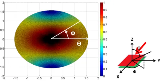
The patch antenna is conformable to any surface, inexpensive, and small size relative to other type of antenna [9][10], then it is used in our system. However, it has the dead zone problem which is shown in Figure 1.1 and 1.2. When we feed a x-direction current into the patch antenna, the normalized amplitude of radiated electric field in each direction shows in Figure 1.1. We observe that there is dead zone in the y-axis, and the patch antenna is not suitable for transmitting the signal in this two directions. If we have a dual-polarized patch antenna, then we can use the y-direction polarization to compensate the dead zone,and it is shown in Figure 1.2. Furthermore, the dual-polarized antenna also provides the low spatial correlations which make our system to enjoy the benefits of MIMO structure, and it will be observed in the simulation results.

We form the multiple antennas to a planar antenna array in the transmit-ter and receiver, and each single element is the dual-polarized patch antenna. It is a dual-polarized planar patch antenna array at the both ends. Based on the antenna structure and indoor 60GHz environment, we want to discuss

Figure 1.1: The normalized amplitude of electric field of the patch antenna with x-direction feeding current

Figure 1.2: The normalized amplitude of electric field of the patch antenna with y-direction feeding current

some problems which are stated in the following section.

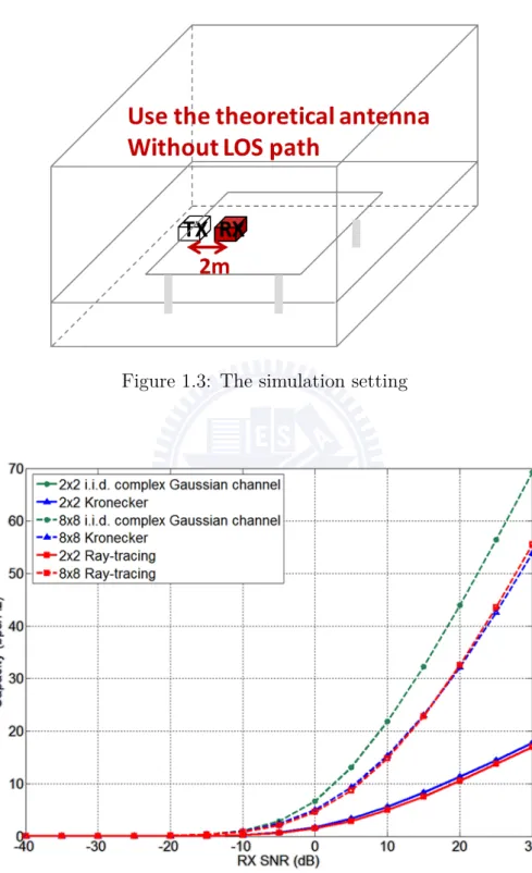
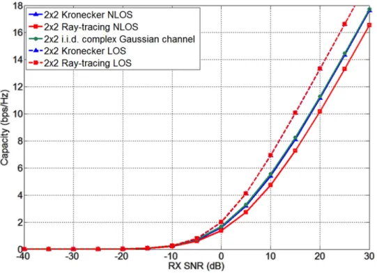
As the mentioned above, we use the dual-polarized antenna to derive the low spatial correlations. Based on the simulation setting as shown in Figure 1.3, Figure 1.4 shows the corresponding results. We can see that our ray-tracing channel model [11] with the 2x2 scheme approaches to 2x2 i.i.d. complex Gaussian channel, but there is a obvious gap for the 8x8 case. It means that our ray-tracing model with the 2x2 scheme has the low spatial correlations, but this is not case for the 8x8 scheme. Therefore, we want to analyze the spatial correlations, and we try to find the factors which affect the spatial correlations. In the beginning, we have a ray-tracing model which needs many parameters of channel and antenna to describe the characteristics of the indoor 60GHz channel and dual-polarized antenna array. From the spatial correlation analysis above, we derive the transmit and receive correlation matrices, and we want to use the two matrices to derive a not only simple but also approximate Kronecker model. We will check whether the corresponding Kronecker model approaches to the ray-tracing model. If we derive an approximate Kronecker model, then we can use a simple channel model to analyze the indoor 60GHz environment and the dual-polarized antenna array effects. There are many works which design the space-time coding and precoding schemes based on the analytic model for dual-polarized MIMO channel [12][13][14].

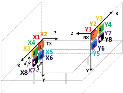
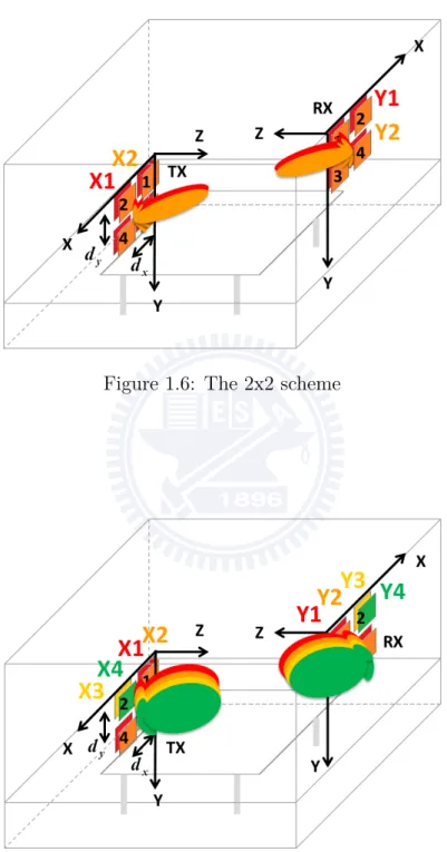
In the MIMO system, if we has multiple data steams, then we may in-tuitively use the spatial multiplexing to send the data steams. In Figure 1.5, we simultaneously send eight data by two polarizations of each antenna respectively, and receiver uses the same scheme to receive the eight data. However, this scheme uses eight expensive A/D and D/A converters. There-fore, we send two data by two polarizations of four antennas respectively, and receiver uses the same scheme. It is shown in Figure 1.6. In this way, it reduces the amount of A/D and D/A to two. Moreover, we can use planar antenna array to form a high-directivity beam. This is the so-called

beam-Figure 1.3: The simulation setting

Figure 1.4: The curves of the capacity versus received SNR for the different channel models

Figure 1.5: The 8x8 scheme

forming technique. Finally, the compromise scheme between the above two. In Figure 1.7, we use four A/D and D/A converters, and we also can use the beamforming by linear array. The directivity is less than 2x2 schems. After the introductions of the three antenna schemes, we want to know which scheme has the best performance under different conditions. Here, we use the channel capacity as a measure. Furthermore, the patch antenna has the dead zone problem as we mentioned above. We want to know whether we can find the more efficient schemes than original three schemes to solve the problem or not.

Figure 1.6: The 2x2 scheme

Chapter 2

Channel Model

We use the capacity as the measure for the three antenna schemes. There-fore, we need an appropriate model which exactly describes the characteris-tics of the indoor 60 GHz channel and dual-polarized antenna array. In this chapter, we give the detailed introduction for channel model. We consider the indoor environment as shown in Figure 2.1. It is a conference room with a table. We limit the transmitter on the table and the receiver above the table. Both of them are equipped with a 2x2 planar dual-polarized antenna array.

Obviously, there are many paths from the transmitter to the receiver, e.g. the line-of-sight (LOS), first order reflections from ceiling, first order reflections from wall, second order reflections from walls, and second order reflections from wall and ceiling. We call the paths which go through the reflection as the non line-of-sight (NLOS) path. The clusters can go through these paths from the transmitter to the receiver. Furthermore, because the reflection surfaces are not ideally smooth in practice, it will cause spreading in the incident and reflection angles of each reflected cluster. Therefore, we assume each reflected cluster is made up of many rays, but the LOS path has the single ray.

There are many antennas in the transmitter and receiver. Referring to [11], the channel impulse response from the u-th baseband transmitter

an-Figure 2.1: The configuration for the indoor environment tenna to the v-th baseband receiver antenna can be written as

hvu(t) = 1 √ L + 1e H v,RX(Φ (0) RX, Θ (0) RX)H (0)_e u,T X(Φ(0)_{T X}, Θ(0)_{T X}) λ 4πd(0)α (0,k) δ(t− T(0)) +√ 1 L + 1 L ∑ i=1 ∑ k eH v,RX(Φ (i) RX + ϕ (i,k) RX, Θ (i) RX+ θ (i,k) RX) H(i)_e u,T X(Φ (i) T X+ ϕ (i,k) T X , Θ (i) T X+ θ (i,k) T X )s (i) λ 4πd(i)α (i,k) δ(t− T(i)− τ(i,k)) (2.1)

It is the summation of many amplitude-scaled and time-delayed Dirac delta functions, which model the characteristics of each ray. i and k are the indices of the cluster and the ray respectively.

eH v,RX(Φ (i) RX+ ϕ (i,k) RX, Θ (i) RX+ θ (i,k) RX )H (0)_e

u,T X(Φ(i)_{T X}+ ϕ(i,k)_{T X}, Θ(i)_{T X}+ θ(i,k)_{T X}) includes

the reflection loss and antenna gains at both ends for the k-th ray of the i-th cluster. (i) , (i) , (i) , (i) are the angle of arrival (AoA) and the

angle of departure (AoD) of the i-th cluster relative to the receiver coordi-nates and the transmitter coordicoordi-nates respectively, where Φ, Θ are azimuth

angle and elevation angle respectively. ϕ(i,k)_RX,θ(i,k)_RX ,ϕ(i,k)_{T X},θ(i,k)_{T X} are the

spread-ing angle of the k-th ray of the i-th cluster relative to the i-th cluster, and each of them is independent and normal distributed. The electrical field vector e(ϕ, θ) =



Eθ(ϕ, θ)

Eϕ(ϕ, θ)



 is composed of two components of the far-zone electric field of the antenna in the specific direction. It equals to the prod-uct of antenna gain G(ϕ, θ) and Jones vector j(ϕ, θ). The Jones vector is the normalized two-dimensional electrical field vector, and it can be used to describe the antenna polarization. We consider not only the theoreti-cal antenna but also a simulated antenna designed with HFSS which is an electromagnetic simulation program. It has the detailed statements in the next chapter. H(i) _{describes the changes of two electric field components of}

the radio wave through the i-th path due to the reflections. Furthermore, because the transmitter and receiver coordinates are inconsistent, H(i) _must

include the transformation matrix from transmitter coordinates to receiver coordinates. For the LOS path, there are no changes for the two electric field components of the radiated wave due to the free space propagation.

H(i) _{equals to the transformation matrix from transmitter coordinates to}

re-ceiver coordinates. For the first order reflection path as shown in Figure 2.2, we have to transform the transmitter coordinates to the incidence plane coordinates, and multiply the first order reflection matrix R₁ =



R⊥1 ξ1

ξ2 R_∥1

 

which models the coupling effect of the two electric field components due to reflection, where the amplitudes of R_⊥1,R_∥1 are independent log-normal

dis-tributed, and the off-diagonal elements have significantly smaller value than

R_⊥1,R_∥1. Finally, we also need to transform the incidence plane coordinates

to the receiver coordinates. H(i) _{of the second order reflection path has the}

similar structure, but there are additional coordinates transformation matrix from the first incidence plane to the second incidence plane and the second

Figure 2.2: First order reflected signal path

order reflection matrix R2=



R⊥2 ξ1

ξ2 R_∥2



, where the amplitudes of R_⊥2,R_∥2

are also independent log-normal distributed. The polarization characteristics may be different for different clusters but are the same for the rays which are in the same cluster. For this reason, H(i) _{is modeled at the cluster level with}

all rays inside one cluster having the same polarization properties. From the statements above, we get

eH

RX(ϕRX, θRX)H(i)eT X(ϕT X, θT X) =

GRX(ϕRX, θRX)GT X(ϕT X, θT X)jRXH (ϕRX, θRX)H(i)jT X(ϕT X, θT X)

where jH

RX(ϕRX, θRX)H(i)jT X(ϕT X, θT X) is the reflection loss.

L is the number of multipath. s(i) is the shadowing factor of the i-th

cluster, and it has the log-normal distribution. LOS path has no shadowing factor. λ

4πd(i) is the path loss of the i-th cluster, whereλis the wavelength and

d(i) is the traveling distance of the i-th cluster. α(i,k) is the gain of the k-th

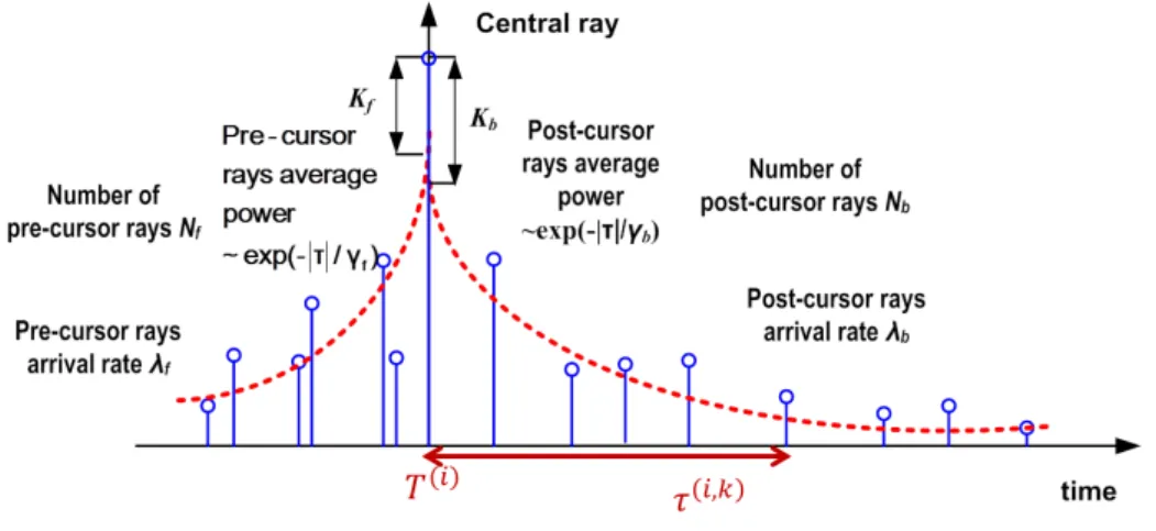
Figure 2.3: Time domain model of the cluster

the uniformly distributed phase. The LOS ray has no uniformly distributed phase. The average amplitudes of the pre-cursor and post-cursor rays decay exponentially as shown in Figure 2.3. T(i) is the time of arrival (ToA) of the

i-th cluster or so-called the central ray. τ(i,k) is the ToA of the k-th ray of the

i-th cluster relative to the central ray. All of the rays in the same cluster can be divided into pre-cursor rays, the central ray, and post-cursor rays based on its ToA. Pre-cursor rays and post-cursor rays are two Poisson processes.

After the generation of SISO channel, we introduce the generation of MIMIO channel. Each pair of transmitter and receiver see the same channel besides the transmitter and receiver antenna patterns. The assumption is based on the half-wavelength antenna spacing.

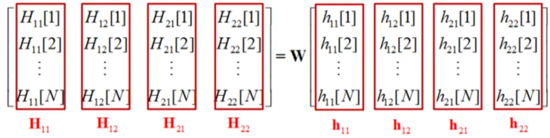
We try to derive the low spatial correlations in the MIMO system by the dual-polarized antenna. Figure 1.4 shows the ray-tracing channel model with the 2x2 scheme has the close curve to 2x2 i.i.d. complex Gaussian channel, but the gap for the 8x8 scheme is larger than 2x2 scheme. Therefore, we analyze the spatial correlations, and we try to find the factors which affect the spatial correlations. The analysis of the spatial correlations is in the following part. Taking the 2x2 MIMO system as an example, we transform the time-domain channel into frequency domain as shown in Figure 2.4, where

Figure 2.4: transform the time-domain channels to frequency-domain chan-nels

H_ij andh_ij are frequency-domain and time-domain channels between the j-th transmit antenna and the i-th receive antenna respectively andWis N-point DFT matrix. We calculate the correlation matrices for the frequency-domain channels. The transmit correlation matrix can be written as

RT X = EH{  HH11 HH 12  [_H11H12]_{} = EH{}  hH11h11 hH11h12 hH 12h11 hH12h12  } (2.2)

due to W is an unitary matrix. Thereby, we can simply calculate the cor-relation matrices in the time domain. It is mentioned above that each pair of transmitter and receiver sees the same channel besides the transmitter and receiver antenna patterns, so the difference between h11 and h12 is the

transmitter antenna pattern. Hence, this difference mainly decides the spa-tial correlations. For the 2x2 scheme as shown in Figure 1.6, the transmitter antenna patterns of the baseband signal X1 and X2 are

e1,T X(ϕ, θ) = AF (ϕ, θ)ex0(ϕ, θ) (2.3) e2,T X(ϕ, θ) = AF (ϕ, θ)ey0(ϕ, θ) (2.4) AF (ϕ, θ) = 4 ∑ i=1 exp_{ȷ(αi+ βi)} (2.5)

which are explained fully in the next chapter. For the 2x2 scheme, the difference of the two transmitter antenna patterns is the polarization. In

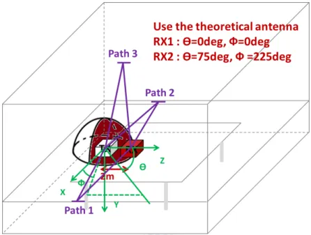
Figure 2.5: The simulation setting

direction polarization. If the two polarizations have a good orthogonality, then the channel coefficients of h12 will be very small relative to h11. In

this case, we will have the low spatial correlations. There are two examples below to verify this idea as shown in Figure 2.5. We fix the location of the transmitter, and the receiver locates in the two directions of the sphere which takes the transmitter as the center with a radius of two meters. When the receiver is in the location 1, the inner product values of all three NLOS paths are 0, and it means a good orthogonality between two polarizations. The corresponding correlation matrices are

RT X =   1 0.0032 0.0032 1   R_RX =   1 0.0210 0.0210 1  

The low spatial correlations explain why the ray-tracing channel model with the 2x2 scheme has the close curve to 2x2 i.i.d. complex Gaussian channel

in Figure 1.4. When the receiver is in the location 2, the inner product values of three NLOS paths are 0.9345, 0.9253, and 0.9181 respectively, and it means a poor orthogonality between two polarizations. The corresponding correlation matrices are

R_{T X} =   1 0.3903 0.3903 1   RRX =   1 0.2517 0.2517 1  

Indeed, we find that good orthogonality of two polarizations provides the low spatial correlations. Furthermore, for the 8x8 scheme as shown in Figure 1.5, the transmitter antenna patterns of the baseband signal X1, X2, X3, X4, X5, X6, X7, X8 are e1,T X(ϕ, θ) =exp{ȷ(α1+ β1)}ex0(ϕ, θ) (2.10) e2,T X(ϕ, θ) =exp{ȷ(α1+ β1)}ey0(ϕ, θ) (2.11) e3,T X(ϕ, θ) =exp{ȷ(α2+ β2)}ex0(ϕ, θ) (2.12) e4,T X(ϕ, θ) =exp{ȷ(α2+ β2)}ey0(ϕ, θ) (2.13) e5,T X(ϕ, θ) =exp{ȷ(α3+ β3)}ex0(ϕ, θ) (2.14) e_{6,T X}(ϕ, θ) =exp_{ȷ(α3+ β3)}ey0(ϕ, θ) (2.15) e_{7,T X}(ϕ, θ) =exp_{ȷ(α4+ β4)}ex0(ϕ, θ) (2.16) e_{8,T X}(ϕ, θ) =exp_{ȷ(α4+ β4)}ey0(ϕ, θ) (2.17)

which are explained fully in the next chapter. The difference between e_{1,T X}

and e_{2,T X} is the polarization, and it is discussed above. e_{1,T X} differs from

e_{3,T X}, e_{5,T X}, e_{7,T X} in a complex exponential term which is caused by the light path difference, and the corresponding correlations are very high. e_{1,T X}

exponen-have a good orthogonal. The corresponding correlation matrices are R_{T X} =                    1 0.0081 0.7739 0.0958 0.8846 0.0090 0.6407 0.1061 0.0081 1 0.0947 0.6026 0.0102 0.4547 0.1052 0.3686 0.7739 0.0947 1 0.0073 0.6541 0.0928 0.8891 0.0097 0.0958 0.6026 0.0073 1 0.0917 0.3852 0.0108 0.4522 0.8846 0.0102 0.6541 0.0917 1 0.0058 0.7541 0.0951 0.0090 0.4547 0.0928 0.3852 0.0058 1 0.0946 0.6051 0.6407 0.1052 0.8891 0.0108 0.7541 0.0946 1 0.0045 0.1061 0.3686 0.0097 0.4522 0.0951 0.6051 0.0045 1                    RRX =                    1 0.0386 0.7411 0.0928 0.8775 0.0217 0.6394 0.0969 0.0386 1 0.1000 0.5900 0.0095 0.4476 0.0921 0.3899 0.7411 0.1000 1 0.0369 0.6285 0.1018 0.8802 0.0209 0.0928 0.5900 0.0369 1 0.1084 0.3815 0.0099 0.4510 0.8775 0.0095 0.6285 0.1084 1 0.0394 0.7578 0.0933 0.0217 0.4476 0.1018 0.3815 0.0394 1 0.0999 0.5918 0.6394 0.0921 0.8802 0.0099 0.7578 0.0999 1 0.0392 0.0969 0.3899 0.0209 0.4510 0.0933 0.5918 0.0392 1                   

We can observe that the high correlations are caused by the light path dif-ference. The high spatial correlations explain why the gap between the ray-tracing channel model with the 8x8 scheme and the 8x8 i.i.d. complex Gaus-sian channel is large in Figure 1.4.

In the ray-tracing model, we need many parameters to describe the chan-nel characteristics. We want to derive a not only simple but also approxi-mate model. Therefore, we can get the corresponding Kronecker model by the correlation matrices and the LOS channel which can be derived from the ray-tracing model. For the Kronecker model, channel matrix can be written as H = M √ K K + 1 H_LOS √ PLOS + M √ 1 K + 1 R1/2_RXHωRH/2_{T X} √ PN LOS (2.20)

R1/2_RXHωRH/2_{T X}, K = _PP_{N LOS}LOS . M is the number of transmitter and receiver

antennas, Hω has i.i.d. zero-mean and unit variance complex normal

dis-tributed entries. RRX,RT X are received and transmitted spatial correlation

matrix. The overall channel can be decomposed into LOS channel and NLOS channel. HLOS is directly derived from ray-tracing model, andRRX,RT X are

introduced above.

Finally, we want to know whether the Kronecker model approximates to the ray-tracing model or not. The simulation setting is shown in Figure 1.3, and we use the theoretical 2x2 scheme. The simulation results are shown in Figure 2.6, and we consider two cases which channel has the LOS path and channel has no LOS path. For the channel with the LOS path, we observe that two models have the nearly same performance. It is caused by the dominant LOS channel, and two models have the same LOS channel. For the channel without the LOS path, there is 1.5 dB SNR gap between two channel models. Therefore, we derive an approximate Kronecker model

Figure 2.6: The curves of received SNR versus capacity for ray-tracing model and Kronecker model

Chapter 3

Antenna schemes

The transmitter and receiver are equipped with 2x2 planar antenna array in our system, and each antenna is a dual-polarized patch antenna. First, we start from the single dual-polarized patch antenna. Here, we consider not only the theoretical antenna but also the simulated antenna, and compare the difference between them. Then, we introduce the overall 2x2 planar antenna array under different antenna schemes.

The theoretical far-zone electrical field of the patch antenna with the x-direction feeding current is [9]

⃗

E(ϕ, θ) = ⃗aϕEϕ(ϕ, θ) + ⃗aθEθ(ϕ, θ) (3.1)

Eθ= ȷ haWakE0exp{−ȷ2π_λr} πr [cos ϕ cos X( sin Y Y )( sin Z Z )] (3.2) Eϕ= ȷ haWakE0exp{−ȷ2π_λ r}

πr [cos θ sin ϕ cos X(

sin Y Y )( sin Z Z )] (3.3) where X = πLa λ sin θ cos ϕ, Y = πWa

λ sin θ sin ϕ, and Z = πha

λ cos θ. The

parame-ters La, Wa, ha are the antenna sizes as shown in Figure 3.1, and we select

La=Wa=1.3mm and ha=0.127mm. k = 2π_λ and E0 is a constant related to

antenna design. Similarly, the electrical field of the patch antenna with y-direction feeding current can be easily derived. As the mentioned above,

Figure 3.1: The illustrated figure for patch antenna

MIMO system. Thereby, we want to know the orthogonality of two polariza-tions for each direction. We take the inner product on two electric fields of two polarizations, and the results are shown in Figure 3.2. We can observe the orthogonality of two polarizations in each direction, and two polarizations have good orthogonality when θ is small.

The simulated dual-polarized patch antenna is based on the design of [John] in electromagnetic simulation program, HFSS. Figure 3.3 is the an-tenna structure and materials, there are x-direction and y-direction feed lines.

h1=0.127mm, h2=0.381mm, h3=0.254mm, r1=r2=1.1mm, w1=w2=1.5mm,

f1=f2=0.8mm, l1=l2=1.25mm, t1=t2=0.43mm. The S-parameters are very

important parameters to judge the designed antenna, and they tell us how much the transmitted power are reflected by the antenna. If the antenna has a very small S-parameters, it means a good power efficiency of the antenna. There are two ports in the simulated dual-polarized antenna, so we have four S-parameters, S11, S12, S21, S22, and all of them are below -15dB at the 60

GHz. The orthogonality of the two polarizations of the simulated antenna can be derived in Figure 3.4, it has a similar trend with the theoretical one. But there are large gaps in many directions. Therefore, we want to compare the simulation results between the theoretical and simulated cases.

Figure 3.2: Inner product for all angle between the electric fields of two theoretical polarizations

Figure 3.4: Inner product for all angle between the electric fields of two simulated polarizations

above. From the antenna array theorem, the electric field of an antenna array which is composed of identical antennas can be written as

e(ϕ, θ) = AF (ϕ, θ)e₀(ϕ, θ) (3.4)

where e0(ϕ, θ) is the electric field of the single antenna which is discussed

above. AF (ϕ, θ) is the array factor.

For the 2x2 scheme as shown in Figure 1.6, the baseband signal X1 is equipped with a 2x2 planar antenna array, so we have

e1,T X(ϕ, θ) = AF (ϕ, θ)ex0(ϕ, θ) (3.5) AF (ϕ, θ) = 4 ∑ i=1 exp_{ȷ(αi+ βi)} (3.6)

wheree_x0(ϕ, θ)is the electric field of patch antenna with the x-direction

kdysin θ sin ϕ. dx and dy are the adjacent antenna spacings in the x and y

di-rections respectively. αi models the ray path difference impact on the i-th

antenna, and βi is the phase of feeding current of i-th antenna. Because

ex0(ϕ, θ) is fixed, we can appropriately select βi such that the amplitude of

array factor has the maximal value in the specific direction. Then, ampli-tude of e_{1,T X}(ϕ, θ) also has the maximal value in the same direction. This

is the so-called beamforming. We assume there is a LOS path in our indoor environment, and intuitively form the beam into the LOS path. e_{i,T X} of the i-th baseband signal has the similar form.

For the 4x4 scheme as shown in Figure 1.7, baseband signal X1 is equipped with a two-element linear antenna array, so we have

e_{1,T X}(ϕ, θ) = AF (ϕ, θ)e_x0(ϕ, θ) (3.7)

AF (ϕ, θ) =exp_{ȷ(α1+ β1)} + exp{ȷ(α4+ β4)} (3.8)

Similarly, we can use the beamforming skill, but directivity is less than 2x2 scheme. We assume there is a LOS path in our indoor environment, and intuitively form the beam into LOS path. e_{i,T X} of the i-th baseband signal has the similar form.

For the 8x8 scheme as shown in Figure 1.5, baseband signal X1 is equipped with single antenna, so we have

e1,T X(ϕ, θ) = AF (ϕ, θ)ex0(ϕ, θ) (3.9)

AF (ϕ, θ) =exp{ȷ(α1+ β1)} (3.10)

Here, we can not use the beamforming skill. This discussion can be applied to the other baseband signals. ei,T X of the i-th baseband signal has the similar

Chapter 4

Simulation results

After the introductions of the indoor 60GHz channel model and antenna structures, we want to compare the capacity between three antenna schemes under different conditions. First, we consider the transmit power impact for three schemes on the capacity. Then, we fix the location of transmitter, and consider the location of receiver impact for three schemes on the capacity. As mentioned above, patch antenna has the dead zone problem, and we try to propose the new schemes that have larger capacity than original three schemes. It will be discussed in the final section.

Before the simulation results, I introduce the capacity calculation here. We transform the time-domain channels into frequency domain, and use the equal power allocation in the transmitter to derive the ergodic capacity C and received SNR ρr as C = EH{ 1 N N ∑ k=1 log₂det(IM + P M σ2 n H[k]H[k]H)} (4.1) ρr= EH{ 1 N N ∑ k=1 P M2_σ2 n T r(H[k]H[k]H))} (4.2)

where N is FFT points, H[k] is the MIMO channel matrix of the k-th

Figure 4.1: The simulation setting

power, σ_n2 is noise power in each receiver antenna. We take average over

frequency tone, and take expectation on the channel matrix.

In this section, we focus on the transmit power issue. The simulation setting is shown in Figure 4.1. Figure 4.2 and 4.3 are plots of transmit power versus capacity and received SNR. From Figure 4.2, we observe that 2x2 scheme has the larger capacity in the low transmit power region and 8x8 scheme is the best in the high transmit power region. More precisely, the threshold for the theoretical antenna is -6.3 dBm, and -4.5 dBm for the simulated antenna. From Figure 4.3, we see that the RX SNR gap between the adjacent two curves is 12 dB. When we want to get the 5 Gbps/Hz which means 9 Gbps transmission rate due to the bandwidth of each subcarrier in 60 GHz radio is approximately 1.8 GHz, 2x2 scheme need -58 dBm, 4x4 scheme need -48.9 dBm, and 8x8 scheme need -39.9 dBm. In other words, 2x2 scheme uses the lowest power to provide the 9 Gbps transmission rate, and it uses the less amount of A/D and D/A converters. Therefore, 2x2 scheme is suitable for the smart phone. In the other hands, if we need the very high data rate which is over 72 Gbps, then 8x8 scheme is the best choice. The 8x8 scheme also uses more amount of A/D and D/A converters. Thereby, 8x8 scheme is suitable for the access point.

Figure 4.2: The curves of transmit power versus capacity for three antenna schemes

Figure 4.3: The curves of transmit power versus received SNR for three antenna schemes

Figure 4.4: The simulation setting

on the capacity for three schemes. Here, we divide the three-dimensional location into distance and direction factors. For the distance factor, we fix the direction of receiver relative to the transmitter, and change the distance with transmitter, as shown in Figure 4.4. For the direction factor, we fix the distance between receiver and transmitter, and change the direction of receiver relative to transmitter, as shown in Figure 4.7.

First, we consider the distance factor, the simulation setting is shown in Figure 4.4, and we fix the transmit power to -10dBm. Figure 4.5 and 4.6 are plots of distance versus capacity and received SNR. The path loss increases when the distance increases such that received SNR and capacity decrease.

Next, we consider the direction factor, the simulation setting is shown in Figure 4.7. Figure 4.8, 4.9, and 4.10 are plots of direction versus capacity for three cases using theoretical antenna. The 2x2 scheme is shown in Figure 4.8, and we can see that capacity decreases as the θ increases. The 4x4 scheme

is shown in Figure 4.9, and we observe that the capacity is smaller than 2x2 scheme in each direction. Furthermore, it has the similar trend with Figure 3.2, i.e., the direction has good orthogonality, and it also has large capac-ity. On the contrary, the poor orthogonality corresponds to small capaccapac-ity. This results are identical with the conclusion which good orthogonality of

Figure 4.5: The curves of distance versus capacity for three antenna schemes two polarizations provides the low spatial correlations and the correspond-ing highly channel capacity. The 8x8 scheme is shown in Figure 4.10, we see that capacity is smaller than 4x4 scheme in each direction. Also, it has the similar trend with Figure 3.2.

We summarize the results so far, it can be observed that the 2x2 scheme has larger capacity than the 4x4 scheme and the 4x4 scheme is better than the 8x8 scheme for -10 dBm power from Figure 4.2. The order will not be changed by the location of receiver. Therefore, transmit power mainly decides the optimal scheme.

In this section, we discuss the dead zone of the patch antenna. When receiver locates in the dead zone of one transmit polarization, we can use the other polarization to transmit the signal. If we only use the strong polarization and focus all the power on this polarization, then we maybe have a better performance than original schemes. Therefore, we have to

Figure 4.6: The curves of distance versus received SNR for three antenna schemes

Figure 4.8: The plot of direction versus capacity for theoretical 2x2 schemes modify the original schemes to get the new schemes which are shown in Figure 4.11, 4.12, and 4.13. Figure 4.11 shows the new scheme by using only the strong polarization from 2x2 scheme, and it is called the 1x1 strong scheme. Similarly, 2x2 strong scheme and 4x4 strong scheme can be derived by using only the strong polarization from 4x4 scheme and 8x8 scheme respectively.

The simulation setting is shown in Figure 4.14 where receiver is located at the dead zone of the transmitter. Figure 4.15 and 4.16 are plots of transmit power versus capacity and received SNR. From Figure 4.15, we observe that 1x1 strong scheme has some benefits in the low transmit power region, and original scheme outperforms the modified schemes in the high power region. From Figure 4.16, we see that the received SNR gap between the new scheme and the old scheme are 6 dB.

Figure 4.10: The plot of direction versus capacity for theoretical 8x8 schemes

Figure 4.12: 2x2 strong scheme

Figure 4.14: The simulation setting

Figure 4.15: The curves of transmit power versus capacity for original and modified antenna schemes

Figure 4.16: The curves of transmit power versus received SNR for original and modified antenna schemes

Chapter 5

Conclusions

Based on the ray-tracing channel model, we analyzed the spatial correla-tions of the 2x2 scheme and the 8x8 scheme. We found that the correlacorrela-tions of the 2x2 scheme are only affected by polarizations, and good orthogonality of two polarizations provides the low correlations. The correlations of the 8x8 scheme are affected by polarizations and a complex exponential term caused by the light path difference, and the complex exponential term causes the high correlations. Moreover, we used the transmit and receive correlation matrices to derive a not only simple but also approximate Kronecker model. Furthermore, we observed that transmit power mainly decides the optimal antenna scheme. More precisely, the 2x2 scheme has the larger capacity in the low transmit power region, and the 8x8 scheme outperforms others in the high power region. Finally, when receiver locates in the dead zone of the transmitter, the 1x1 strong scheme can provide some benefits in the low transmit power region.

Bibliography

[1] H. Yang, P. F. M. Smulders, and I. Akkermans, “On the design of low-cost 60-GHz radios for multigigabit-per-second transmission over short distances,” IEEE Communications Magazine, vol. 45, no. 12, pp. 44–51, Dec. 2007.

[2] C. R. Anderson and T. S. Rappaport, “In-building wideband partition loss measurements at 2.5 and 60 GHz,” IEEE Trans. on Communications, vol. 3, no. 3, pp. 922–928, May 2004.

[3] “WirelessHD,” available at http://www.wirelesshd.org/index.html. [4] “IEEE 802.15 WPAN Millimeter Wave Alternative PHY Task Group

(TG3c),” available at http://www.ieee802.org/15/pub/TG3c.html. [5] “IEEE 802.11ad: Very High Throughput 60 GHz,” available at http://

www.ieee802.org/11/.

[6] “WiGig White Paper: Defining the Future of Multi-Gigabit Wireless Communications,” July 2010, available at http:// wirelessgigabital-liance.org/specifications/.

[7] E. Torkildson, U. Madhow, and M. Rodwell, “Indoor millimeter wave mimo: Feasibility and performance,” IEEE Trans. on Wireless Communi-cations, vol. 10, no. 12, pp. 4150–4160, Dec. 2011.

“Ca-wireless channel at 60 GHz,” in Proc. IEEE Vehicular Technology Confer-ence (VTC) Spring, Dublin, Ireland, 22-25 April 2007.

[9] C. A. Balanis, “Antenna theory: Analysis and design,” 1997, New York, Singapore: Wiley.

[10] Shyh-Jong Chung, “Lectures of antenna design for wireless communica-tion,” 2008.

[11] Alexander Maltsev et al, “Channel models for 60 ghz wlan systems,” in

IEEE doc. 802.11-09/0334r8. IEEE 802.11 TGad, May. 2010.

[12] C. Oestges, B. Clerckx, M. Guillaud, and M. Debbah, “Dual-polarized wireless communications: from propagation models to system perfor-mance evaluation,” Wireless Communications, IEEE Transactions on, vol. 7, no. 10, pp. 4019 –4031, october 2008.

[13] Taejoon Kim, B. Clerckx, D.J. Love, and Sung Jin Kim, “Limited feed-back beamforming systems for dual-polarized mimo channels,” Wireless Communications, IEEE Transactions on, vol. 9, no. 11, pp. 3425 –3439, november 2010.

[14] Yabo Li, Haiquan Wang, and Xiang-Gen Xia, “On quasi-orthogonal space-time block codes for dual-polarized mimo channels,” Wireless Com-munications, IEEE Transactions on, vol. 11, no. 1, pp. 397 –407, january 2012.