Translating fab cycle time and output targets into production control requirements for tool groups

Translating Fab Cycle Time and Output Targets into Production

Control Requirements for Tool Groups'

Ming-Der Hut, Shi-Chung Chang+

*Laboratory of Control and Decision, Department of Electrical Engineering, National Taiwan University

+ Graduate Institute of Industrial Engineering and Dept. of Electrical Engineering, National Taiwan University

Abstract

Throughput rate and cycle time are two of the major production targets of a fab. As a fab is often operated under distributed production flow control, the overall delivery specifications can be achieved only when individual tool groups are operated to meet appropriate local performance requirements. In this paper, a control parameter extraction methodology is proposed to establish explicit relationship between production targets of a fab and local flow control parameters in terms of mean rates and upper bounds on variations of input processes for each tool group. These parameters can further be utilized to derive managerially tangible requirements for cycle times and wafer-in-processes and to create guidelines for distributed production control leading to the desired delivery specifications. Validations over two benchmark fab models demonstrate that our approach is mostly within 95% of accuracy and requires less than one millisecond of CPU time.

1. Introduction

Cycle time and output rate are two major production targets for a fab. As a fab is often operated under distributed production flow control, output targets should be translated into shop floor performance requirements based on fab characteristics so that individual controllers may operate locally to meet the overall output specifications. How to translate output rate and cycle time related targets into control parameters of individual tool groups or production steps has been a significant and challenging research topic of production flow control due to the complexity of fabrication processes, many heterogeneous tools, re-entrant nature of process flows, and various uncertainties.

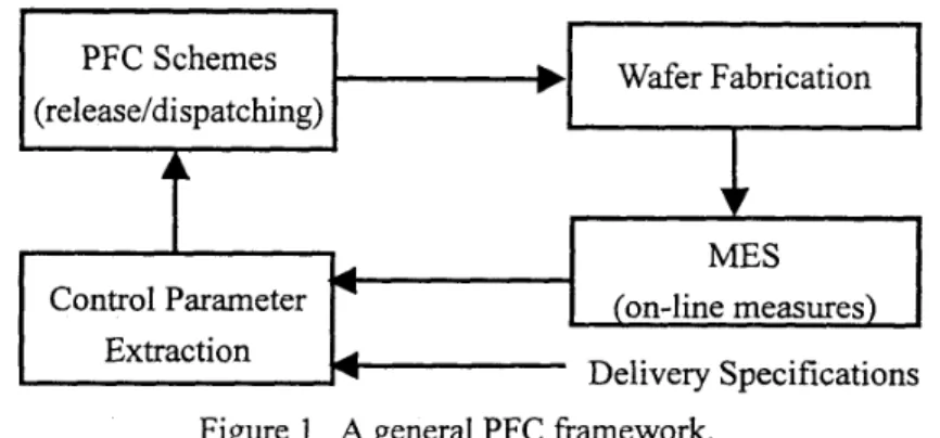
Hu and Chang (1999) summarized a general framework of production flow control (PFC) in a fab as depicted in Figure 1. In this framework, manufacturing execution system (MES) collects the measurable information from the shop floor of a fab. PFC parameters are then periodically extracted from both measured fab status data and the given delivery specifications, and are fed into the PFC scheme. Line

managers or a PFC computer executes the control activity calculatedrecommended by the PFC scheme to regulate wafer release and dispatch wafers to individual tools for fabrication. Wafer Fabrication PFC Schemes (release/dispatching)

A

MES control Parameter on-line measures)

I

Delivery Specifications

Figure 1 A general PFC framework.

To successfully implement the PFC framework, Hu and Chang (1998) proposed a control parameter extraction methodology to facilitate effective PFC schemes. In the methodology, a fab is modeled as a re-entrant, open queueing network (OQN) with flows of various part types aggregated into one. The aggregated, re-entrant OQN is analyzed by using a class of approximate, decomposition methods. The decomposition methods decompose an OQN into individual network nodes and use two types of parameters to characterise the stochastic input, service and output processes of each node: one describing the rate and the other describing the variability. Various stationary network performance measures can then be derived based on these two types of parameters. On top of the re-entrant OQN model and the decomposition method, a backward analysis (BA) is designed to derive target mean rates and squared coeficient of variation (SCV) bounds of input processes of individual nodes with given delivery specifications in a systematic way.

In this paper, we apply the BA to translating mean cycle time and output rate targets into PFC requirements such as average production rate and bounds on wafer-in-process (WIP) level at each tool group. Validations of BA adopt the 60-step, 12-tool-group fab models of Lu et al. (1 994) and Lin (1 996), where the latter

extends the former to two product types. Application of BA to each model requires less than one millisecond of CPU time on a Pentium-III300 personal computer. Comparisons of BA results with those of simulation show that differences are mostly within 5% at both node and system levels. Complexity analysis of BA warrants its fast re-calculation with respect to changes of system capacity and delivery specifications. Both the accuracy and computing efficiency of BA support its potential for real-sized flow control applications.

To be successfully applied in real fabs, BA must be applicable to various delivery specifications. And the input information that BA requires should be extracted from easily measurable shop floor data. In this paper, we also show that BA can be applied to many significant delivery specification items such as mean cycle time, cycle time variance and bound of output rate.

The remainder of the paper is organized as follows. developed in Section 2.

specifications.

results over the two benchmark re-entrant lines are given in Section 4. Section 5 concludes the paper.

BA of the OQN model is Section 3 then describes ow design of BA for other delivery Validation Finally, Potential applications to PFC of fabs are also addressed.

2.

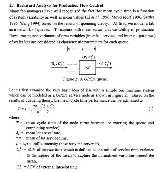
Backward Analysis for Production Flow Control

Many fab managers have well recognized the fact that mean cycle time is a function of system variability as well as mean values (Li et al. 1996, Meyersdorf 1996, Sattler 1996, Wang 1994) based on the results of queueing theory. At first, we model a fab as a network of queues. To capture both mean values and variability of production flows, means and variances of time variables (inter-lot, service, and inter-output times) of wafer lots are considered as characteristic parameters for each queue.

I+--

T - 4

Figure 2 A GVGA queue.

Let us first examine the very basic idea of BA with a simple one machine system which can be modeled as a GYGA service node as shown in Figure 2. Based on the results of queueing theory, the mean cycle time performance can be estimated as

zp

c: +c;

T = z + -

1 - p 2 where:

T = mean cycle time of the node (time between lot entering the queue and completing service),

&

= mean lot arrival rate, z = mean of lot service time,

p = &Z= traffic intensity (how busy the server is),

Cf = SCV of service time which is defined as the ratio of service time variance to the square of the mean to capture the normalized variation around the mean,

C: =

scv

ofextemd inter-lot time.

Let the delivery specifications of the simple system for output rate is d and the upper

bound of cycle time is T, then when the queue is in a steady state, the desired lot arrival rate should be

and the associated SCV of the inter-lot time can be calculated as

If the wafer release is controlled to meet the target rate and to restrain its inter-lot time SCV no greater than the value calculated in Eq. (2), then the output rate and mean cycle time of this system should meet the given delivery specifications.

i ' External:

1

i

I

' I * Tool Group 2

___* flow of part type A + flow of part type B

--__--___-_-

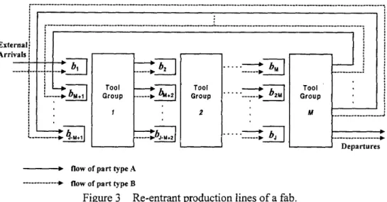
Figure 3 Re-entrant production lines of a fab.

Our BA extends the basic idea described above. Consider a fab as a series of shared and failure-prone service nodes, each corresponding to a group of identical tools illustrated in Figure 3, where there are M tool groups and J different production steps. There contains three elements in each service node: an arrival process, a service process and a queue, where the arrival process of a service node is affected by the operation and characteristics of upstream nodes while the service process by those of

the service node itself. We approximately characterize a processes by two statistical parameters, i.e., mean rate and inter-lot time SCV and assume that the service discipline at each node is First-Come-First-Serve (FCFS). In analyzing the queueing model, the departure process of one service node is a combination of its arrival and service processes and it becomes a part of the arrival of a downstream node. Mathematical relationship between the arrival process parameters of one service node and the departure process parameters of upstream service nodes can then be established based on the process flow. In conjunction with the arrival-departure relationship of each service node (Eq. (2)), two sets of linear equations are then established to describe the relationship of mean and SCV parameters among processes of all nodes in the queueing network. Given output rate and mean cycle time requirements, our BA derives the associated extemdintemal arrival processes parameters by solving the two sets of linear equations. Interested readers may refer to Hu and Chang (1999) for more details.

In the analysis above, FCFS is assumed as the service discipline. In manufacturing practice, various service disciplines are usually designed for individual nodes to result in better output performances than simply using FCFS. In our derivations, the

bounds on input processes of individual nodes under the FCFS service discipline may intuitively serve as upper bounds for real applications.

3.

Many frequently considered delivery specifications can be derived from mean and

SCV parameters of service and input processes. As the theoretic foundation of BA is based on these first and second order statistical parameters, BA can be easily extended to many other delivery specifications. For example, since mean output rate and inter-output time SCV of the output process are important operational goals for on-time delivery, let us consider output rate, d, and upper bounds of inter-output time SCV,

c,Z,

as the output targets.

BA for Other Delivery Specifications and PFC Applications

To capture the very basic idea, we also examine the one machine system modeled as a

GI/G/l service node shown in Figure 2. Based on the results of queueing theory, the inter-lot time SCV can be estimated by

c;

=(l-p)Ce‘+pC,z.

Then

with

some mathematical manipulation, the desired lot release rate should be and the associated SCV of the inter-lot time can be calculated as

de = d

This system output performance shall be guaranteed to meet the given delivery specifications if the wafer release is controlled to meet the target rate and to restrain its inter-lot time SCV no greater than the value calculated in Eq. (3).

Application to Production Flow Control

Applications of queueing models and approximation techniques to PFC mostly exploit the following two basic results from single server node analysis:

First order relation (Little’s formula) L = d W

where: d = average lot arrival rate to the service node

FV=

average time a lot stays in the service node L = average number of lots in service node; Second order relation

zp

c,2+c,’

EW =-

I - p

2

EW= average time in waiting queue. where: C,’ = inter-lot time SCV

available, one can utilize them to calculate the distributed measurable production performance metrics such as cycle time and WIP at individual tool groups (Whitt

1983, 1993). Remarks

In manufacturing practices of fabs, there have been various PFC schemes (Leachman 1994, Li et al. 1996, Wu et al. 1998). Many of them use target levels and bounds of WIPs andor cycle times as the measures to control because such data is easily accessible fiom the shop floor and is managerially tangible to operators. Although the PFC parameters derived by BA are mean rates and SCV bounds of input processes for each tool group, they can be further utilized to derive other tangible requirements, such as cycle time and WIP. BA may therefore provide these existing PFC schemes of re-entrant lines with effective calculation of control parameters and facilitate their realization.

4.

Numerical and Simulation Results

To validate the BA by comparing its numerical approximations with discrete event simulation results, two exemplary fab models of Lu et al. (1994) and Lin (1 996) are adopted. The former is a single-product fab model while the latter extends it to two product types for investigation of multiple product-type effect. A C language-based discrete event dynamic system (DEDS) simulator (Hsieh et al. 1998) is used for simulation. Our validation first applies the BA procedure to derive all the means and SCVs of inter-lot times of a fab model. The derived external arrival parameters

(Ae

,Cf ) are set as inputs to the simulation model. Simulation results of internal process parameters are then compared with the derived ones and simulated output

performance measures are compared with the specified ones.

In the simulation study of each model, there are six simulation runs. The basic entity of the production flow is a lot, which consists of 24 semiconductor wafers. Each simulation run begins with an empty line and ends at the 114,OOOth lot departure out of the line. The simulation of the first 14,000 lot departures serves as a warm-up period. The succeeding simulation is partitioned into 20 intervals (batches) for collecting statistics such as the mean and variance of cycle time and WIP. Statistics of individual batches are then averaged over all the 120 batches of the six simulation TuflS.

4.1 Single-Product Fab

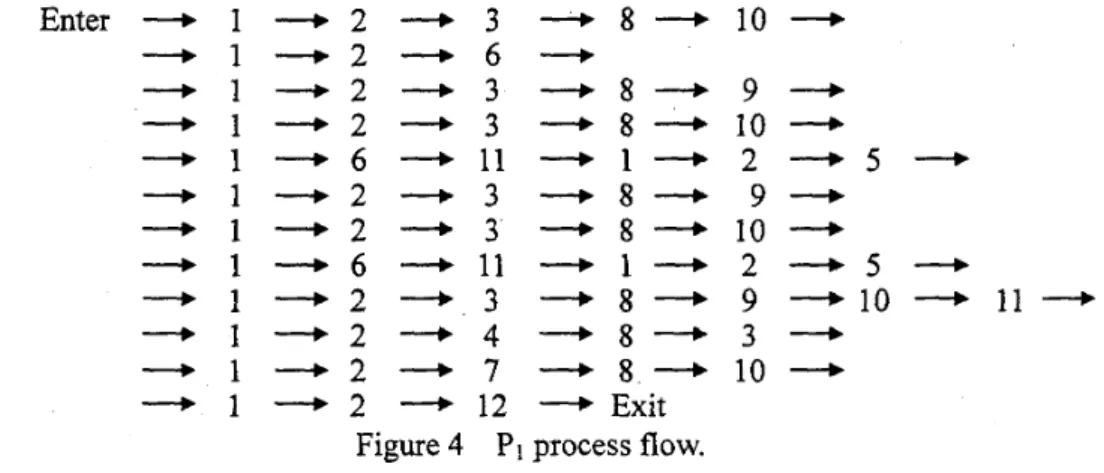
The model of Lu et al. (1994) consists of 60 production stages, 12 different tool groups (TGs) and a total of 40 tools. There is only one part type. Its sequence of processing steps and the TG used by each step are given in Figure 4. Tools are subject to random failures, and each failed tool requires a random repair time.

All

the times to failure, times to repair, and processing times have exponential distributions with various values of mean time to failure (MTTF), mean time to repair

(MTTR) and mean processing time (MPT). Table 1 lists the basic information of the model. Delivery specifications of this example are set as statistical performance metrics frequently considered in fabs:

(1) desired output rate d = 0.52 l o t s h , and (2) mean cycle time target T = 3 83.2466 hours,

where the given output rate equals to the wafer release rate of Lu et al. (1994) and the mean cycle time bound is based on our simulation of the line under the selected release rate. The output rate of the line demands for an average tool loading over

30%, and TGs 9 and 11 are two capacity bottlenecks with 96.0% loading intensity. 1 - 1 - 1 - 1 - 1 - 1 - 1 - 1 - 1 - 1 - 1 - 1 - 2 - 3 - 8 - 2 - 6 - 2 - 3 - + 8 + 2 - 3 - 8 - 6 - + 1 1 - 1 - 2 - 3 - 8 - 2 - 3 - 8 - 6 - 1 1 + 1 + 2 - 3 - 8 - 2 - 4 - 8 - 2 - 7 + 8 - - + 2 ----+ 12 + Exit

Figure 4 PI process flow. Results of applying BA to this example are obtained in

10 ---, 9 - 10

-

2 - 5

-

9 - 10

-

2 - 5 + 9 -10

-

1 1 - 3 - 10

-

0.5495 millisecond of CPU

time on a Pentium-I1/300 personal computer. Table 2 lists the derived requirements for mean and upper bounds on SCVs of arrival processes to individual TGs. The derived extemal arrival parameters

(de

,C,') = (0.52, 0.99) are then input to our

discrete simulation.

Figures 5 and 6 contrast node level performance in cycle times and WIP levels derived by BA and simulation respectively. Although the estimates of SDWIP at the TG level have large deviations, the maximum deviation in term of lots at individual

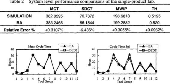
TGs is only 1.369. These results confirm that the nodal arrival parameters calculated by using BA can be accurately transformed into the measurable performance requirements such as mean and variance of nodal cycle time and WIP. Table 2 shows that system level performances in MCT, SDCT, MWIP

and

output rate (TH) by simulation are close to the delivery specifications. It clearly implies that the re-entrant line achieves the target TH and MCT when arrival parameters are controlled to match the performance requirements calculated by BA.

Table 2 System level uerformance comuarisons of the sindemoduct fab. ~ ~~ ~ " A

MCT SDCT MWIP TH SIMULATION 382.0595 70.7372 198.681 3 0.51 95 BA 383.2466 66.1844 199.2882 0.520 Relative Error % +0.3107% -6.436% +0.3055% +0.0962% 40 30 -6- DEDS

g

20 3: 10 0 1 2 3 4 5 6 7 8 9 1 0 1 1 1 2 1 2 3 4 5 6 7 8 9 1 0 1 1 1 2 Tool Group T Tool Group

Figure 5 Cycle time mean and standard deviation of the single-product fab.

-B- DEDS 20 15

j

10 5 0 1 2 3 4 5 6 7 8 9 1 0 1 1 1 2 1 2 3 4 5 6 7 8 9 1 0 1 1 1 2

Tool Group Tool Group

Figure 6 WIP (in Lots) mean and standard deviation.

4.2 Two-Product Fab

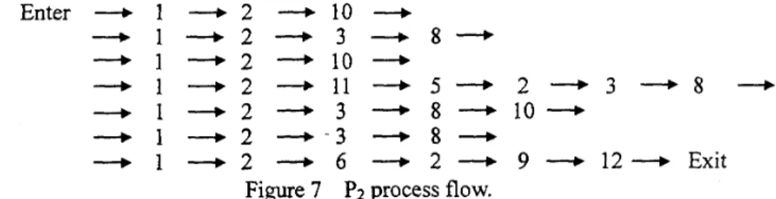
This model extends the previous fab model to two product types, say PI and P2. Process flows of PI and P2 (Lin 1996) are shown in Figures 4 and 7 respectively. In this model, TGs 5 and 9 contain only one tool and are shared by P1 and P 2 , and TGs 4

and 7 are needed only for the processing of PI. All the time related random variables are again assumed of exponential distributions with various values of MTTF, MTTR and MPT. Tables 4 specifies parameters of individual TGs. The product-mix ratio between PI and P2 is 3:2. Delivery specifications are set as:

(1) desired output rate d = 0.63 13 l otsh, and (2) mean cycle time target T = 170.6 12 hours,

and the specified cycle time bound is from simulation of the line. Note that the MPT in Table 3 has been modified such that the capacity bottleneck is TG 11 with a loading intensity of 92.536% under the desired output rate.

Enter -+ 1 -+ 2 -+ 10 + + 1 - 2 ----+ 3 + 8 - - 1 - 2 - 1 0 - -+ 1 - 2 -+ 11 + 5 - 2

-

3 - 8 + - + 1 - + 2 + 3 - + 8 - - - + 1 0 * + 1 + 2 + - 3 + 8 +

-

1 --.* 2 ----* 6

-

2 + 9 --+ 12- Exit

Figure 7 P2 process flow.

Application of BA to this model again takes 0.5495 millisecond CPU time. In specific, the external arrival parameters

(de,

C: ) set for simulation study are (0.63 13, 0.998).

Table 4 System level Derformance comDarisons of the two-Droduct fab.

~ ~~~~~~~~~~~ ~~

SIMULATION 214.17 106.09 0.3783 0.252

BA 212.88 107.21 0.3788 0.2525

1 .O529% 0.1232% 0.2099%

Relative Error Oh -0.606%

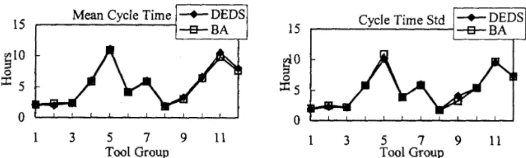
Figure 8 provides the performance comparisons of the cycle time mean and standard deviation at the node level between BA and simulation. These results suggest that

local cycle time performance requirements also can be accurately estimated from calculated nodal arrival parameters in the two-product system. System level performance results of each product type appear in Table 4. This table demonstrates that the relative errors of individual products in delivery performance are all within 5%. It also confirms that the aggregate delivery specifications can be achieved in a

two-product model when arrivals follow the arrival requirements calculated by BA. Compared with the results presented in Section 4.1, it is observed that class aggregation procedure does not significantly affect the CPU time in this example.

Mean Cycle Time +DEDS

4 BA

15 1 _{15 1} Cycle Time Std _{-B- BA}

I I

1 3 5 7 9 11 1 3 5 7 9 1 1

Tool Group Tool Group

Figure 8 Cycle time mean and standard deviation of the two-product fab. Discussions

BA is a near accurate and computationally efficient way to translate delivery specifications into distributed flow control requirements. It is observed that the calculated WIP and cycle time are mostly within 95% of accuracy at both TG and system levels in our application of BA to the above two fab models.

It is also observed that it takes less than one millisecond of CPU time to apply BA to above-mentioned benchmark re-entrant lines. Specifically, the main computation load of BA lies in solving the two sets of linear equations to obtain required arrival parameters of individual nodes. After aggregation, the dimension of the linear equations depends only on the number of different tool groups but not on the number of tools, the number of production steps, or the number of part types. There are many existing and efficient algorithms for solving such linear equations. Such computation efficiency warrants the application of BA to real-sized fabs and to fast re-calculations with respect to the changes of system capacity and delivery specifications.

5.

Concluding Remarks

In this paper, we developed a method of translating delivery specifications into PFC

parameters for tool groups in terms of mean rates and upper bounds on SCVs of input processes for re-entrant production lines of fabs. A re-entrant, multiple part type production line with failure prone tools was first modeled as an aggregated OQN. By combining decomposition-based techniques, we designed BA to derive PFC

parameters from two sets of linear equations with mean cycle time and output rate as the delivery specifications. We also showed that delivery specifications can be selected from other frequently used production performance metrics. We applied BA to two benchmark fab models and each application took less than one millisecond of CPU time. Validations demonstrated that the differences between BA and simulation were mostly within 95% of accuracy at both tool group and system levels.

Both the accuracy and computing efficiency of BA support its potential for real fabs. Results of BA were utilized to derive the performance requirements of both the aggregate and per part type cycle time and WIP. These measurable performance requirements can be used to design control charts for guiding production flow control, where the target is the mean and the control limits are set at level with respect to the standard deviation.

References

Hu, M.-D., and Chang, S.-C., 1998, Translating fab cycle time and throughput spe’cifications into stepwise flow control requirements. Pro. of International Symposium on Semi. Manu$, Tokyo, Japan, pp.38 1-384.

Hu, M.-D., and Chang, S.-C., 1999, Translating delivery specifications into distributed production flow requirements for re-entrant lines. Submitted to International Journal of Production Research.

Hsieh, B.-W., Hu, M.-D., Chen, C.-H. and Chang, S.-C., 1998, DEDS-Discrete event dynamic system simulator. Dept. Elec. Eng., National Taiwan University, Taipei, Taiwan, ROC.

Leachman, R., 1994, Production Planning and Scheduling Practice Across the Semiconductor Industry. TechnicaI Report, ESRC 94-29/CSM-18, U.C. Berkeley, CA.

Li, S., Tang, T., and Collins, D. W., 1996, Minimum inventory variability schedule with application in semiconductor fabrication. IEEE Trans. Semi. Manu$, 9, Lin, C.-Y., 1996, Shop flow scheduling of semiconductor wafer fabrication using real-time feedback control and predictions. Ph.D. dissertation, Dep. IEOR,

University of California at Berkeley, USA.

Lu, S. H., Ramaswamy, D., and Kumar, P. R., 1994, Efficient scheduling policies to reduce mean and variance of cycle-times in semiconductor manufacturing plants. IEEE Trans. Semi. Manu$, 7,374-388.

Meyersdorf, D., 1996, Cycle time reduction. Lecture notes of Workshop on Layout PIanning and Cycle i’ime Reduction for Semi. Manu$, Hsin-Chu, Taiwan.

Sattler, L., 1996, Using queueing curve approximations in a fab to determine productivity improvements. in Proceedings of the 7th Annual IEEEh’EMI Advanced Semiconductor Manufacturing Conference and Workshop, Cambridge, Wang, F., 1994, Consideration for manufacturing control systems. Key Note Speech Whitt, W., 1983, The queueing network analyzer. BelI System Technical Journal, 62, Whitt, W., 1993, Approximations for the GI/G/m queue. Prod. and Opera. Manage. , 2, Wu

,

K.-L., Wei, K., Tsai, C.-Y., Chang, S.-C., Wang, N.-J., Tsai, R.-L., Liu, H.-P.,

1998, TSS: a daily production target setting system for foundry fabs. Pro. of International Symposium on Semi. Manu$, Tokyo, Oct. 7-9, 1998, pp.75-78.

145-149.

MA, pp. 140-145.

Note of I994 Semiconductor Manufacturing Workshop, Hsin-Chu, Taiwan. 2779-2815.