What is a good g?

(1)

INTELLIGENCE 18, 23 I-258 (1994)

EDITORIAL

What Is a Good g?

ARTHUR R. JENSEN Universi~ of Calfornia, Berkelq

LI-JEN WENC Nutiorzul Taiwan University, Taipei

We have examined the stability of psychometric R, the general factor in all mental ability tests or other manifestations of mental ability, when g is extracted from a given correlation matrix by different models or methods of factor analysis. This wab investigated in simulated correlation matrices, in which the true g was known exactly, and in typical empirical data consisting of a large battery of diverse mental teats. Theoretically, some methods are more appropriate than others for extracting R. but in fact g is remarkably robust and almost invariant across different methods of analysis, both in agreement between the estimated g and the true R in simulated data and in similarity among the K factors extracted from empirical data by different methods. Although the near-uniformity of g obtained by different methods would seem to indicate that, practically speaking, there is little basis for choosing or rejecting any particular method, certain Factor models qua models may accord better than others with theoretical considerations about the nature ofg. What seems to us a reasonable strategy for estimating g. given an appropriate correlation matrix, is suggested for consideration. It seems safe to conclude that, in the domain of mental abilities, K is not in the least chimerical. Almost any g is a “good” R and is certainly better than no 8.

Contrasting Views of g

The chimerical nature of i: is the rotten core of Jensen’s edifice, and of the entire hereditarian school.

So stated Stephen J. Gould in his popular book The Mismeusure of Man (198 I, p. 320). Gould railed against the “reification” of g, implying that g theorists regard it as a “thing’‘-a “single,” “innate,” “ineluctable,” “hard” “object,” to quote his own words. In Gould’s view, g is nothing more than a mathematical artifact, representing no real phenomenon beyond the procedure for calculating it. He argued that the x factor, its size and pattern of factor loadings in each of the

For their helpful comments on the first draft of this article, we are grateful to Richard Harshman, the late Henry F. Kaiser, John C. Loehlin, and Malcolm J. Ree. Special thanks are due to John B. Carroll for his trenchant critique of the penultimate draft. Thanks also to Andrew L. Comrey for providing us with the computer program for his Tandem factor analysis.

Correspondence and requests for reprints should be sent to Arthur R. Jensen, School of Educa- tion, University of California, Berkeley, CA 94720.

(2)

tests in a given battery of diverse tests administered to a particular group of persons can differ widely, or even be completely absent, depending on the psy- chometrician’s arbitrary choice among different methods of factor analysis. In Gould’s words, “Spearman’s g is not an ineluctable entity; it represents one mathematical solution among many equivalent alternatives” (p. 3 18).

In marked contrast to Gould’s position, the most recent and comprehensive textbook on theories of intelligence, by Nathan Brody (1992), states

The first systematic theory of intelligence presented by Spearman in 1904 is alive and well. At the center of Spearman’s paper of 1904 is a belief that links exist between abstract reasoning, basic information-processing abilities, and academic performance. Contemporary knowledge is congruent with this belief. Contempo- rary psychometric analyses provide clear support for a theory that assigns fluid ability, or g, to a singular position at the apex of a hierarchy of abilities. (p. 349)

The g Factor as a Scientific Construct

Jensen has commented on Gould’s argument in detail elsewhere (Jensen, 1982), noting that Gould’s strawman issue of the reification of g was dealt with satisfac- torily by the pioneers of factor analysis, including Spearman (1927) Burt (1940) and Thurstone ( 1947). Their views on the reification of g are entirely consistent with modern discussions of the issue (Jensen, 1986; Meehl, 1991), in the light of which Gould’s reification bugaboo simply evaporates. From Spearman (I 927) to Meehl (1991), the consensus of experts is that x need not be a “thing”-a “single, ” “hard, ” “object’‘-for it to be considered a reality in the scientific sense. The g factor is a wtzsrrwt. Its status as such is comparable to other constructs in science: mass, force, gravitation, potential energy, magnetic field, Mendelian genes, and evolution, to name a few. But none of these constructs is a “thing.” According to Gould, however, “thingness” seems to be the crucial quality without which g is, he says, “chimerical,” which is defined by Webster as “existing only as the product of unrestrained imagination: unreal.”

Existence and Reality of g

Various mental tests measure different abilities, as shown by the fact that, when diverse tests are given to a representative sample of the general population, the correlations between the tests are considerably less than perfect. Most of the correlations are typically between + .20 and + .X0. In batteries of mental tests, correlations that are very near zero or even negative can usually be attributed to sampling error. The fact that, in large unrestricted samples of the population, the correlations are virtually always positive can be interpreted to mean that the tests all measure some common source of variance in addition to whatever else they may measure.

This common factor was originally hypothesized by Francis Galton (1869), but it was Charles Spearman (1904) who actually discovered its existence and

(3)

WHAT IS A GOOD g’? 233

first measured it empirically. He called it the general factor of mental abilities and symbolized it as g. Since Spearman’s discovery, hundreds of factor analyses of various collections of psychometric tests have yielded a g factor, which, in unselected samples, is larger than any other factor (uncorrelated with g) that can be extracted from the matrix of test intercorrelations. In terms of factor analysis per se, there is no question of the “existence” of x, according to Carroll (1993). But a most crucial fact about g that makes it so important is that it also reflects a phenomenon outside the realm of psychometric tests and the methodology of factor analysis, as demonstrated by the substantial correlations of g with certain behavioral and biological variables that are conceptually and methodologically external to either psychometric or factor analytic methodologies (Jensen, 1987a,

1987b). For example, among the various factors in every battery of tests that have been examined with respect to external validity, g is by far the largest source of practical validity, outweighing all other psychometric factors in predicting the outcomes of job training, job performance, and educational achievement (Jensen, 1992a, 1993a; Ree & Earles, 1992).

Also, g is related to reaction times and their intraindividual variability in various elementary cognitive tasks (Jensen, 1992b, 1992~). Brain-evoked poten- tials are correlated much more with g than with other factors (reviewed in Jensen, 1987a). The heritability (proportion of genetic variance) of scores on various tests is directly related to the tests’ g loadings, and g accounts for most (all, in some cases) of the genetic covariance in the matrix of correlations among tests (Cardon, Fulker, DeFries, & Plomin, 1992; Humphreys, 1974; Jensen, 1987a; Pedersen, Plomin, Nesselroade, & McClearn, 1992). The effects of genetic dom- inance, as reflected in the degree of inbreeding depression of scores on subtests of the Wechsler Intelligence Scale, involve g much more than the Verbal and Performance factors (Jensen, 1983). The complementary phenomenon, namely, the effect size of heterosis (outbreeding) on test scores, is related to the tests’ x loadings (Nagoshi & Johnson, 1986). Hence, there can now be little doubt that g is a solid scientific construct, broadly related to not only psychometric variables but also real-life behavior, as well as to electrophysiological indices of brain activity and to genetic phenomena.

Stability of g Loadings Across Different Test Batteries

Various tests, when factor analyzed together, typically differ from one another in their g loadings. We can ask: To what extent is any particular test’s g loading a function of the particular mix of other tests included in the factor analysis? If g were really chimerical or capricious, we might expect a test’s g loading to be wildly erratic from one factor analysis to another, showing a relatively high loading when factor analyzed among one set of tests and a relatively low loading when analyzed in a different set, even though the method of factor analysis and the subject sample remained constant.

(4)

assumptions about the nature, number, and diversity of the tests that are factor analyzed, it has not yet been subjected to extensive empirical investigation. The largest empirical study to date was conducted by the late Robert L. Thorndike ( 1987). He began with 65 highly diverse tests used by the U.S. Air Force. Forty- eight of the tests were selected to form six nonoverlapping batteries, each composed of eight randomly selected tests. Each of the 17 remaining “probe” tests was inserted, one at a time, into each of the six batteries. Each battery, therefore, was factor analyzed 17 times, each time containing a different probe test. (The g was extracted as the first principal factor.) The six g loadings obtained for each of the 17 probe tests were then compared with one another. Although there was considerable variation among the g loadings of the 17 probe tests, their g loadings were highly similar across the six different batteries: The average correlation of the probe tests’ g loadings across the six batteries was .85. (The stability of g loadings would inevitably increase as the number and diversity of the tests in each battery increased.) In brief, the tests maintained approximately the same g loadings when factor analyzed among different random sets of diverse tests.

EXTRACTION OF g BY DIFFERENT TYPES OF ANALYSIS

There seems little question that g is a valid construct and is of great interest and importance in differential psychology. But there is the problem that several different types, models, or methods of factor analysis are widely used in contemporary research. The central question to be addressed here concerns the choice of method for best representing the general factor, or g, in a correlation matrix (henceforth abbreviated as R-matrix) of mental tests. How much does g vary across different methods of factor analysis? Do some methods represent g better than others? If different methods applied to the same data yield different gs, which g is the “good” g? One might even ask whether these questions can be given theoretically and empirically coherent answers.

First, however, one might ask why psychometricians and researchers on hu- man mental abilities should be concerned with the choice of methods for estimating the g factor in a given battery of tests. There are at least four main reasons why one might want a good g.

I. One might wish to select from among a large battery of diverse tests some much smaller number of tests that have the largest g loadings. The composite score from these g-selected tests would, of course, provide a better estimate of g than some randomly or subjectively chosen subset of the entire battery, provided, of course, that the g-selected tests are also sufficiently varied in their loadings on other, group, factors besides g, such that loadings on the different orthogonal (i.e., uncorrelated) group factors are approximately balanced, thereby tending to “cancel” one another in the composite score.

(5)

WHAT IS A GOOD g? 235

2. One may wish to obtain g-factor scores of individuals, a factor score being a weighted linear combination of the person’s z scores on a number of tests that maximizes the composite scores’ correlation with the g factor and mini- mizes its correlation with other factors. Methods for estimating factor scores are explicated by Harman ( 1976, chap. 16).

3. One might want to follow Spearman, who originally gained some insight into the psychological nature of g by rank-ordering various tests in terms of their g loadings and analyzing the characteristics of the tests in terms of this ordering (Spearman & Jones, 1950). The method is still used, for example, to infer the specific characteristics of various experimental cognitive tasks that make them more or less g loaded, by decomposing their total variance in a factor analysis that includes a battery of typical g-loaded psychometric tests (e.g., Carroll, 1991, Table 6).

4. One may correlate the column vector of g loadings of a number of tests with a parallel column vector of the same tests’ correlations with some external variable, to determine whether the external variable involves g, as distinct from other factors. The method has been used, for example, to test whether the lowering of test scores by the genetic phenomenon of inbreeding depression is the result of its effect on g or on other factors (Jensen, 1983). The method has also been used to study the highly variable size of the average black-white difference across various tests (e.g., Jensen, 1985, 1993b; Naglieri & Jensen, 1987). This technique, which might be termed the met/z- od of correlated vectors, is analytically more powerful than merely correlat- ing the measures of some external variable with g-factor scores, because the vector of correlations (each corrected for attenuation) of a number of different tests with the external variable must necessarily involve a particular factor, for example g, if the vector of the tests’ loadings on the factor in question is significantly correlated with the vector of the tests’ correlations with the external variable. The method may be applied, of course, to investi- gating whether g (or any other factor) is related to any given external variable. The method, however, is quite sensitive to the rank order of tests’ factor loadings and, therefore, may give inconsistent results for different methods of factor analysis if the rank order of the tests’ loadings on the factor of interest is much affected by the type of factor analysis used. Some Basic Definitions

Our present purpose is not to discuss theoretical notions about the nature of g, that is, its causal processes, but to consider g only from the standpoint of factor analysis per se. Several points are called for:

1. Not all general factors are g. For instance, there is a very large general factor in various measures of body size (height, weight, leg length, arm length, head circumference, etc.), but this general factor is obviously not g. The g factor applies only to measures of mental ability, objectively defined.

(6)

An ubility is identified by some particular conscious, voluntary behavioral act that can be objectively assessed as meeting (or failing to meet) some clearly defined standard. An ability is considered a mentul ability if individual differences in sensory acuity and physical strength or agility constitute a negligible part of its total variance in the general population.

2. The general factor of just uny set of mental tests is not necessarily g, although it will necessarily contain some x variance. The factor analytic identi- fication of g requires that the set of tests be diverse with respect to type of information content (verbal, numerical, spatial, etc.), mode of stimulus input (visual, aural, tactual, etc.), and mode of response (verbal, spoken, written, manual performance, etc.). Regardless of the method of factor analysis, the “goodness” of the g extracted from a set of tests administered to a representative sample of the general population is a monotonic function of the (a) number of tests, (b) test reliability, (c) number of different mental abilities represented by the various tests, and (d) degree to which the different types of tests are equally represented in the set. These criteria can be approximated preliminary to performing a factor analysis.

The g factor varies across different sets of tests to the extent that the sets depart from these criteria. Just as there is sampling error with respect to statistical parameters, there is psychometric sampling error with respect to g, because the universe of all possible mental tests is not perfectly sampled by any limited set of tests. If consistently good g “marker” tests, such as Raven’s Progressive Ma- trices, have been previously well established in many factor analyses that observed these rules, then, of course, it is an efficiently informative procedure to include such tests as g markers in the analysis of a set of new tests whose factori- al composition is yet unknown. The above rules for identifying g originally can then be somewhat relaxed in determining the x loadings of new tests.

The fact that increasing the number of tests in a set causes nonoverlapping sets of diverse tests to show increasingly similar and converging g factors suggests that the obtained g factors are estimates or approximations of a “true” g, in the sense that, in classical test theory, obtained scores are estimates of true scores. Under the necessary assumption that R was extracted from a limited but random sample of the universe of all mental tests, the correlation between the obtained g (x,) and the true g (R,) is given by the formula proposed by Kaiser and Caffrey ( 1965) also explicated by Harman (1976, pp. 230-23 I):

where n is the number of tests and A is the eigenvalue of the first principal component of the R-matrix. The formula has no practical utility, however, unless a universe of tests can be precisely specified and randomly sampled. But it is theoretically useful for showing that the reliability or generalizability of g is

(7)

related both to the number of tests in the factor analysis and to the eigenvalue of the first principal component of the R-matrix, which is intimately related to the average correlation among the tests. Kaiser (1968) has shown that the best estimate of the average correlation (i) in a matrix is (with n and A as defined above):

,-h-1 n- 1.

3. “Spearman’s g” and “psychometric g” are both terms used in the literature, often synonymously. But a distinction should be noted. Spearman’s g is correctly associated only with his famous two-factor theory, whereby each mental test measures only g plus some test-specific factors (and measurement error). Spear- man’s method of factor analysis, which is seldom if ever used today, can properly extract g only from an R-matrix of unit rank, that is, a matrix having only one common factor. Such a matrix meets, within the limits of sampling error, Spear- man’s criterion of vanishing tetrad differences. This tests whether the R-matrix has only one common factor. Proper use of Spearman’s particular method of factor analysis must eliminate any tests that violate the tetrad criterion before extracting g (Spearman, 1927, App.). If Spearman’s method of factor analysis is applied to any matrix of rank > 1 (i.e., more than one common factor), the various tests’ g loadings are contaminated and distorted to some degree. And Thurstone ( 1947, pp. 279-28 1) has clearly shown that no group factors can properly be extracted from the residual matrix that remains after extracting g from an R-matrix of rank > 1 by Spearman’s method. Therefore, it is best that the term “Spearman’s g” be used only to refer to a general factor extracted by Spearman’s method from an R-matrix of unit rank. A g factor extracted from an R-matrix with rank > 1, by any method of multiple factor analysis, is best called “psychometric g.” We will refer to it henceforth simply as g, without the adjective.

4. Orthogonal rotation of multiple factors, or the transformation of factors (rotation of factor axes), keeping them orthogonal (uncorrelated first-order factors), is an absolutely inappropriate factor analytic procedure in the ability domain, except possibly when used as a stepping-stone to an oblique rotation (i.e., correlated first-order factors such as promax). Yet one commonly sees orthogonalized rotations used in many factor analyses of mental tests, usually by means of Kaiser’s (1958) varimux, a widely available computerized analytic method for orthogonal rotation of factors. It is the most overly used and inappropriately used method in the history of factor analytic research. Varimax accomplishes remarkably well its explicit purpose, which is to approximate Thurstone’s criterion of simple structure as nearly as the data will allow, while maintaining perfectly orthogonal factors. But in order to do so, varimax necessarily obliterates the general factor of the matrix. In fact, varimax (or any other method of orthogonal rotation of the first-order factors, except Comrey’s Tandem I criterion (Comrey, 1973, p. 185) mathematically precludes a g factor. If there is, in fact, a general

(8)

factor in the R-matrix, as there normally is for ability tests, varimax scatters all of the g variance among the orthogonally rotated factors, and hence no R factor can appear in its own right. When the g variance is large, as it usually is in mental tests, varimax “tries” to yield simple structure but conspicuously fails. That is, on each of the first-order factors, many of the loadings that should be near-zero under the simple-structure criterion are inflated by the bits of g that are scattered about in the factor matrix. When there is, in fact, a general factor in the correlation matrix, simple structure can be closely approximated only by oblique rotation, whereby the g variance goes into the correlations between the factors. A higher order, or hierarchical, g can then be extracted by factor analyzing the correlations among the oblique factors.

5. Theoretically, all g loadings are necessarily positive. Any negative loading is either a statistical fluke or a failure to reflect a variable (e.g., number of errors) so that superior performance is represented by higher scores (e.g., number correct).

Major Methods for Extracting g

Several different methods for representing the general factor of an R matrix are seen in the modern psychometric literature. (All except the LISREL model are explicated in modem textbooks on factor analysis, e.g., Harman, 1976.) Each has certain advantages and disadvantages with respect to representing g. The methods mentioned next are listed in order of the number of decisions that depend upon the analyst’s judgment, from least (principal-components analysis) to most (hierarchical analysis). All these methods are called “exploratory factor analysis” (EFA), except LISREL. Although LISREL is usually used for “confirmatory factor analysis” (CFA), to statistically test (or “confirm”) the goodness- of-fit of a particular hypothesized factor model to the data, it can also be used as an exploratory technique.

Principal Components. Principal components (PC) analysis is a straightfor- ward mathematical method that gives a unique solution, requiring no decisions by the analyst. The procedure begins with unities (i.e., the standardized total variance of each variable) in the leading diagonal of the R-matrix. It has the advantages that (a) it calls for no decisions by the analyst, and (b) the calculation of the first principal component (PC I), which is often interpreted as x, does not depend on the estimated number of common factors in the matrix or the estimated communalities of the variables. Although the PC1 has often been used to represent g, it has three notable disadvantages when used for this purpose. 1. Not the common factor variance alone, but the total variance (composed of

common factor variance plus uniqueness) of the variables in the R-matrix, is included in the extracted components. The unwanted unique variance is scattered throughout all the components, including PC1 This unique vari-

(9)

WHAT IS A GOOD R? 239

ante, which is not common to any two variables in the matrix, adds, in effect, a certain amount of “error” (or nonfactor) variance to the loadings of each component, including the PC1 , or g.

2. Because of this, the proportion of the total variance in all of the variables that is accounted for by PC1 can considerably overestimate g.

3. But by far the most serious objection to PC analysis, from the standpoint of estimating g, is that every variable in the matrix can have a substantial posi- tive loading on PC 1, even when there is absolutely no general factor in the R matrix, in which case the g as represented by PC1 is, of course, purely a methodological artifact.’ One can create an artificial R-matrix such that it has absolutely no general factor (i.e., zero correlations among many of the variables), and PC analysis will yield a substantial PC 1. However, if there is actually a general factor and it accounts for a large proportion of the variance in the matrix, PC1 usually represents it with fair accuracy, except for the reservations listed in Points 1 and 2. The reason is that PC analysis is really not formulated to reveal common factors. Rather, the column vector of PC 1 (i.e., the loadings of the variables on PC 1) can be properly described as the vector of weights that maximizes the sample variance (individual differences) of a linear (additive) composite of all of the variables’ standardized (z) scores. This unique property of PC 1 does not necessarily insure that PC 1 represents a general factor. All told, there seems little justification for using PC1 as a measure of g. Certainly it cannot be used to prove the existence of g in a given R-matrix.

Principal Factors (PF). PF analysis is one form of common factor analysis, in the sense that, ideally, it analyzes only the variance attributable to common factors among the variables in the R-matrix. The procedure requires initial estimates of the variables’ communalities (h2) in the leading diagonal of the R- matrix. (Such a matrix is termed a reduced R-matrix.) The most commonly used initial estimates of the h2 values are the squared multiple correlations (SMCs) between each variable and all of the remaining variables. The initial estimates of h2 can be fine-tuned closer to the optimal values by iteration of the PF analysis, by entering the improved estimates of the communalities derived from each re- factoring, until the h2 values stabilize within some specified limit. Communality estimation based on iteration also depends on determining the number of factors in the matrix, for which there are several possible decision rules, the most popular being the number of eigenvalues > 1 in the R-matrix. This procedure, how-

‘The error of interpreting PC1 as a general factor even when there are nonsignificant correlations between some variables that have substantial loadings on PC1 has probably been a rather common occurrence in studies of the relation between individual differences in performance on elementary cognitive tasks and psychometric R. J.B. Carroll has pointed out a clear example of this error in an article by Jensen (1979).

(10)

ever, tends to overestimate the number of factors, at least when the correlations among variables are generally quite small (Lee & Comrey, 1979) but at times it underestimates the number of factors, particularly if the factors are correlated. (Critiques of the eigenvalues > 1 criterion and suggested alternative solutions are offered by Carroll, 1993, pp. 83#:, Cliff, 1988, 1992, and Tzeng, 1992.)

Thus, two kinds of decisions in PF analysis are up to the individual analyst: the methods for determining the number of factors and for estimating communalities. Unlike PC analysis, which is a purely mathematical procedure with no decisions to be made by the analyst, PF analysis involves some subjective judgment. Of course, PF analyses by different analysts will give identical solutions to a given R-matrix if they both follow the same decision rules. If they follow different rules, however, there is generally less effect on the first principal factor (PFI) than on any other features of the solution. And if, indeed, a general factor exists in the R-matrix, a PFI is a better estimate of it than a PC1 , because PFl represents only common factor variance, whereas the PC1 loadings are somewhat inflated by unwanted variance that is unique to each variable.

But PF analysis has exactly the same major disadvantage as PC analysis: Even when there is absolutely no general factor in the R-matrix, the PFI can have all the appearance of a large general factor, with substantial positive loadings on every variable. Thus PFl is not necessarily g, but it is defined essentially as the vector of weights (derived from the reduced R-matrix) that maximizes the variance of a linear composite of the variables’ z scores. However, if a true x exists and accounts for a substantial proportion of the variance in the R-matrix, PFI typically represents it with fair accuracy, but only if there is good psychometric sampling, that is, sufficient diversity in the types of tests included in the analysis. To the extent that tests of certain primary abilities are over-represented relative to others, PFI will not properly represent g, because it will contain variance con- tributed by the overrepresented group factors in addition to x.

It should be noted also that both PC1 and PFI are more sensitive than some other methods (e.g., hierarchical factor analysis) to what we have termed psy- chomefric sampling error. That is, the variables in the R-matrix may be a strong- ly biased selection of tests, such that some non-g factor is overrepresented. As Lloyd Humphreys (1989) has nicely stated, ‘*Over-sampling of the tests defining one of the positively intercorrelated group factors biases the first factor [PFl] or component [PCI] in the direction of the over-sampled factor” (p. 320). For instance, if the R-matrix contained three verbal tests, three spatial tests, and a dozen memory tests, the PC 1 and PFl could possibly represent as much a memory factor as the x factor or at least be an amalgam of both factors. One of the advantages of a hierarchical factor analysis is that its g is less sensitive to such “psychometric sampling error” than is either PC 1 or PFl , because a hierarchical g is not derived directly from the correlations among tests but from the correlations among the first-order, or group, factors, each of which may be derived from differing numbers of tests (> 2).

(11)

WHAT IS A GOOD g” 241

Hierarchical Factor Analysis. The highest order common factor derived from the correlations among lower order (oblique) factors in an R-matrix of mental tests is an estimate of g. The first-order factors are usually obtained by PF analysis (although PC is sometimes used), followed by some method of oblique rotation (transformation) of the factor axes, which determines the correlations among them. Hierarchical factors can be thought of in terms of their level of generality. Each of the first-order factors (also called primary or group factors) is common to only a few of the tests; a higher order factor is common to two or more of the first-order factors and, ipso facto, to all of the tests in which they are loaded. The g factor, at the apex of the hierarchy, is typically a second-order factor, but it may emerge as a third-order factor when a great many diverse tests are analyzed (e.g., Gustafsson, 1988). The g is common to all of the factors below it in the hierarchy and to all of the tests. A hierarchical analysis assumes the same rank of the R-matrix as a PF analysis. That is, it does not attempt to extract more factors than properly allowed by the rank of the matrix; it simply divides up the existing common factor variance in terms of factors with differing generality. The total variance accounted for by a PF analysis and a hierarchical analysis is exactly the same.

Hierarchical analysis involves the same decisions by the analyst as PF analysis and, in addition, a decision about the method of oblique rotation, of which there are several options, aimed at optimal approximation to Thurstone’s criteria of “simple structure” (Harman, 1976, chap. 14).

A hierarchical analysis can be orthogonalized by the Schmid-Leiman procedure (Schmid & Leiman, 19.57), which makes all the factors orthogonal (i.e., uncorrelated) to one another, both between and within levels of the hierarchy. This generally yields a very neat structure. In recent years, it has become probably the most popular method of exploratory factor analysis in the abilities domain. Wherry ( 1959) has provided a mathematically equivalent, but conceptually more complex, procedure that yields exactly the Schmid-Leiman solution, without need for oblique rotation.

LISREL Methods of Factor Analysis. Linear Structural Relations (LISREL) is a highly flexible set of computer algorithms for performing confirmatory factor analysis (as well as other kinds of analyses of covariance structures) based on maximum likelihood (ML) estimation (Jbreskog & Sorbom, 1988). (Bentler,

1989, provided a computer program, EQS, that serves the same purpose but is more user friendly for those not versed in the matrix algebra needed for model specification in LISREL.) The essential purpose of confirmatory factor analysis is to evaluate the goodness of fit of a hypothesized factor model to the data. A specific model, or factor structure, is hypothesized, based on theoretical considerations or on prior exploratory factor analysis of the set of tests in question. The model is specified in LISREL (or Bentler’s EQS). From the empirical data (R- matrix), the computer program simultaneously calculates ML estimates of all the

(12)

free parameters of the model consistent with the specified constraints. It also calculates an index of goodness-of-fit of the model to the data. If the fit is deemed unsatisfactory, the model is revamped and tested again against the data, to obtain a better fit, if possible. But a satisfactory fit to any reasonably parsi- monious model is not always possible.

The flexibility of the LISREL program allows it to simulate the distinctive results of virtually every type of factor analysis, provided the model is properly specified; hence it can be used to test the goodness-of-fit of factor models derived by any standard method of factor analysis including those previously described. Also, prior estimates of communalities are not required; they emerge from the LISREL analysis, but the accuracy of the calculated h’ values depends on how correctly the factor model has been specified.

Also, prior estimates of commuralities are not required; they emerge from the LISREL analysis, but the accuracy of the calculated h2 values depends on how correctly the factor model has been specified.

Typical Factor Models

Diagrams of some of the main types of factor models that have figured in x theory will help to elucidate our subsequent discussion. Each model needs only a brief comment at this point.

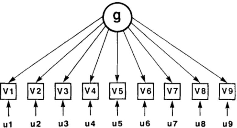
Model S. Figure 1 shows the model of Spearman’s 2-factor theory, in which each variable (V), or test, measures only x and a component specific (s) to that variable. In addition to s, each variable contains a component resulting from random measurement error (e). The sum of their variances, s2 + e2, constitutes the variable’s utziquenes.~ (G), that is, the proportion of its total variance that is not common to any other variable in the analysis. The correlation between the unique element and V is the square root of V’s uniqueness, or II. This is the simplest of all factor models, but it is appropriate only for correlation matrices that contain only a single common factor. As other common factors besides x are usually present in any sizable battery of diverse tests, Model S (for Spearman) does not warrant further detailed discussion.

Model T. Figure 2 shows the idealized case of Thurstone’s multiple-factor model, with perfect simple structure. The criterion of simple structure is that each of the different group factors (FI , F2, etc.) is significantly loaded in only certain groups of tests, and there is no general factor. In reality, simple structure allows each variable to have a large, or salient, loading on one factor and relatively small or nonsignificant loadings on all other factors. (This could be represented in Figure 2 by faint or dashed arrows from Fl to each of the variables besides Vl to V3, and similarly for F2 and F3.) Kaiser’s varimax rotation of the principal factors (or principal components) is a suitable procedure for this model. However, the model is appropriate only when there is no general factor, only a

(13)

WHAT IS A GOOD x? 243

~1 u2 u3 u4 u5 u6 u7 u6 u9

Figure 1. Model S. The simplest possible factor model: A single general factor. originally proposed

by Spearman as a two-jhctw model, the two factors being the general factor (g) common to all of the variables (V) and the “factors” specific to each variable, termed specificifv (s). Each variable’s

w~iqueness (u) comprises 5 and measurement error.

number of nonsignificantly correlated group factors. Model T mathematically excludes a g factor, even when a large g is present in the data. A good approximation to simple structure, which is necessary to justify the model, cannot be achieved by varimax when g is present. Therefore, Model T is not considered further. It has proved wholly inappropriate in the abilities domain. The same is true for any set of variables in which there is a significant general factor. In such cases, to perform orthogonal rotation, such as varimax, as some analysts have done in the past, and then to argue on this basis that there is no g factor in the battery of tests is an egregious error.

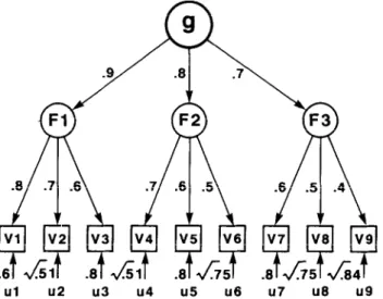
Model A. An ideal hierarchical model is shown in Figure 3. The numerical values shown on the paths connecting the factors and variables in Model A are

ul u2 u3 u4 u5 u8 u7 u8 u9

Figure 2. Model 7: A multiple-factor model with three independent group factors (Fl, F2, F3), without a ,q factor common to all of the variables, originally proposed by Thurstone.

(14)

ul u2 u3 u4 u5 u6 u7 u8 u9

Figure 3. Model A. A hirrarchid model, in which the first-order, or RKXL~, factors (F) are correlated, giving rise to a second-order factor g. Variables (V) are correlated with g only via their correia- tion with the three first-order factors. (The particular correlation coefficients attached to each of the paths were used to generate the correlation matrix in Table I .)

the linear correlations between these elements. Note that each variable (V) is loaded on only one factor (F). Note also that, in a true hierarchical model, the R loading of each variable depends on the variable’s loadings on the first-order factor (e.g., Fl) and on the factor’s loading on g. For example, the g loading of V 1 is .8 X .9 = .72. One can also residualize the variables’ loadings on the first- order factors; that is, the K is partialed out of F, leaving the variable’s residualized loading on F independent of g. The residualized loading is (1 - g* - u*)l/*, where g is the variable’s x loading of V I on Fl is [ 1 - (.72)* - (.6)*]‘/* = .3487. The result of this procedure, carried out on all the variables, is known as the Schmid-Leiman ( 1957) orthogonalization of the factor hierarchy. It leaves all the factors orthogonal to one another, between and within every level of the hierarchy.

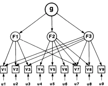
Model B. This might be called a mixed hierarchy. As shown in Figure 4, some of the variables are loaded on more than one of the group factors. This can happen when a test reflects two (or more) distinct factors, such as a problem that involves both verbal comprehension and numerical ability. In this case, the correlation between a compound variable and g has more than one path through the group factors. For example, in Figure 4, the g loading of Vl depends on the correlations represented by the sum of the two paths g + Fl -+ V 1 and g + F3 --$ VI. An important question is whether this complication seriously affects the estimate of g when it is extracted by the usual methods. All of the factors in

(15)

WHAT IS A GOOD g‘? 245

ul u2 u3 u4 u5 u6 u7 u6 u9

Figure 4. Model B. A hierarchical model, as in Model A. but one in which most of the variables (V) are factorially complex, each being loaded on two (or more) of the three group factors (F).

Model B can be orthogonalized by the Schmid-Leiman transformation, as in Model A.

Model C. Shown in Figure 5 is essentially what Holzinger and Swineford (1937) called the bi-jiicfor model. Note that it is not a hierarchical model, because g (which is necessarily loaded in all of the variables) does not depend on the variables’ loadings on the group factors. (While the correlation matrices corresponding to Models A and B, as depicted in Figures 3 and 4, are of rank 3, the

ul u2 u3 u4 u5 u6 u7 u6 u9

Figure 5. Model C. A &j&for model, originally proposed by Holzinger, in which each variable (V) is loaded on one of the three group factors (F) and is also loaded on g, but the variables’ R loadings are not constrained by their loadings on the group factors (as in the case of Models B and C). Variables’ correlations with F and with g are independent of one another.

(16)

correlation matrix corresponding to Model C is of rank 4.) First, g is extracted from the original correlation matrix in such a way as to preserve positive manifold (i.e., all positive coefficients) in the residual matrix; and then, from the residual matrix, the group factors are extracted in an orthogonalized fashion. (The computational procedure is well described in Harman, 1976, but this model is now most easily solved with LISREL or Bentler’s EQS, but only if one can determine the factor pattern by inspecting the R-matrix or by a prior EFA to determine which loadings are to be constrained to zero.)

Model LI. Not shown here, this is the same as Model C, except that some of the variables are loaded on more than one group factor, as in Model B. Again, one wonders how this complication might affect the g extracted by the bi-factor method.

Agreement Between True g and Estimated g Our aims here are as follows:

1. To create four artificial, but fairly typical, correlation matrices derived from Models A, B, C, and D with specified parameters in each model. Hence, we know exactly the true g loadings of each variable. It could be argued that if we created a variety of sufficiently atypical correlation matrices, their g factors might be a good deal less similar to one another than is typically found for mental test data. But every form of measurement in science necessarily has certain boundary conditions, and to go beyond them has little theoretical relevance. As we will later show, certain matrices can be simulated even in such a way that no g factor can properly be extracted. But, unless one can demonstrate the existence of such grossly atypical matrices in the realm of mental tests, they are hardly relevant to our inquiry.

2. To factor analyze each of these artificial matrices by each of six different methods that are commonly used for extracting g.

3. To look at the degree of agreement between the known true g and the estimated x by calculating both the Pearson correlation and the congruence coefficient2 between the column vector of true g loadings and the corresponding vector of estimated g loadings.

‘The congruence coefficient, with a range of possible values from ~ I to + I, is a measure of factor similarity (Harman, 1976, p. 344). Theoretically, the congruence coetkicnt closely approxi- mates the Pearson correlation between g factor scores (see Gorsuch, 19X3, p. 285), but empirically the congruence coefficient, on average, probably overestimates slightly the correlation between the factor scores. At least. in a large-scale study of the stability of 8 across different methods of estimation (Ree & Earles, 199 I), a comparkon of 91 congruence coefficients and the corresponding correlations between factor scores showed a mean difference of .013 (i.e.. ,997 ~ ,984).

(17)

WHAT IS A GOOD ~1 247

The entire procedure is here illustrated only for Model A; the same procedure was applied to all the other models, but, to conserve space, only the third step is shown for them.

Table 1 is the correlation matrix generated from the numerical values shown for Model A in Figure 3.3 The true factor structure and true values of all the factor loadings and other parameters are shown in Table 2. Model A and each of the other models are treated the same way. Table 3 shows the correlations and congruence coefficients between the vector of true g loadings and the corresponding estimated g loadings obtained by six different methods, which are la- beled as follows:

SL:PF(SMC). Schmid-Leiman (SL) orthogonalized hierarchical factor analysis, starting with a principal factor (PF) analysis with squared multiple correlations (SMC) as estimates of the communalities in the leading diagonal (not iterated).

SL:IPF. Same as the first method, but with the PF analysis iterated (I) to obtain more accurate estimates of the communalities.

CFA:HO. Confirmatory factor analysis (CFA), based on maximum likelihood (ML) estimation, using the LISREL program and specifying a hierarchical (H), orthogonalized (0) model.

CFA:g + 3F. CFA as in the previous method, using LISREL, and specifying Holzinger’s bi-factor model (Model C in Figure 5).

Tandem I. Comrey’s (1967) Tandem I method of factor rotation for extracting g, a method so devised as not to extract a g unless there is truly a general factor in the matrix, by the criterion that any two variables positively correlated with one another must be loaded on the same factor.

PF(SMC). g is represented by the first (unrotated) principal factor from a PF analysis with squared multiple correlations (SMC) in the leading diagonal (not iterated). This is the simplest and most frequently used method for estimating g, but, as noted previously, it runs the risk of spuriously showing a g when there really is no g in the matrix. All the other methods listed here cannot extract a g factor unless it actually exists in the correlation matrix. The most salient feature of Table 3 is the overall high degree of agreement between true g and estimated g. The overall average correlation and congruence 3The method for calculating the zero-order correlations between variables (i.e., the R-matrix) from the values shown in Model A (in Figure 2) is most simply explained in terms of path analysis, where the given values are the path coefficients between the observed variables (VI, V2, etc.) and the latent variables, or factors (FI, F2, F3, and g). The correlation between any two variables, then, is the product of the path coefficients connecting the two variables. For example, the correlation between VI and V2 is .8 X .7 = .56, and the correlation between VI and V7 is .8 X .9 X .7 x .6 = .3024.

(18)

TABLE 1

Correlation Matrix Derived From Model A

VI v2 v3 V4 V5 V6 v7 V8 v9 Vl v2 V3 V4 v5 V6 Vl V8 v9 5600 4800 4032 3456 2880 3024 2520 2016 5600 4800 4200 4200 3528 3024 3024 2592 2520 2160 2646 2268 2205 1890 I764 1512 4032 3528 3024 4200 3500 2352 I960 1568 3456 3024 2592 4200 3000 2016 1680 1344 2880 2520 2160 3500 3000 1680 1400 1120 3024 2646 2268 2352 2016 1680 3000 2400 2520 2205 I890 1960 1680 1400 3000 2016 1764 1512 1568 1344 1120 2400 2000

Nore. Decimals omitted

coefficients are ,943 and ,998, respectively. It is also apparent that the various methods of analysis yield more or less accurate estimates, depending on how well a given method matches a particular model. Three of the methods, for example, estimate the x in Model A with perfect accuracy, but these same methods are less accurate than certain others for Model B (a “mixed” hierarchy). Judging from the row means in Table 3, the PF(SMC) shows the best overall agreement between true and estimated g, having the highest mean correlation (.966) and highest mean congruence coefficient (.998) and the smallest standard deviations for both. If PF(SMC) had been iterated to obtain more accurate communalities, it probably would have averaged even higher agreement with true g. (However,

TABLE 2

Orthogonalized Hierarchical Factor Matrix for Model A Factor Loadings

Variable

2nd Order 1st Order Communality Uniqueness

g Fl F2 F3 hZ uz VI .72 .3487 0 0 .64 .36 V2 .63 .3051 0 0 .49 .51 v3 .54 .2615 0 0 .36 .64 v4 .56 0 .42 0 .49 .51 v5 .4x 0 .36 0 .36 .64 V6 .40 0 .30 0 .25 .75 VI .42 0 0 .4284 .36 .64 V8 .35 0 0 .3570 .25 .75 v9 .28 0 0 .2856 .I6 .X4 Var. 2.2882 ,283 ,396 .3925 3.36 5.64 %a Var. 25.42 3.15 4.40 4.36 37.33 62.67

(19)

WHAT IS A GOOD g? 249

TABLE 3

Correlations and Congruence Coeffkients Between True g Loadings in Four Different Models and g Loadings Obtained by Four Different Analytic Methods

Model Method A B C D M SD SL:PF(SMC) SL:IPF CFA:HO CFA:g + 3F Tandem I PF(SMC) .9990 (.9996) I 0000 (I .OOOO) I 0000 ( I .OOOO) I .oooo ( I 0000) .9977 (.9996) .9979 (.9995) .7780 (.9958) .7823 (.9953) .7649 (.9952) .7959 (.9957) .8307 (.9969) .9055 (.9978) .9971 (.9989) .9979 (.9990) .9914 (.9984) I .oooo ( I 0000) .9740 (.9983) .9870 (.9987) .9705 (.9965) .9641 (.9964) .9730 (.9968) .9X52 (.9984) .9578 (.9960) ,973 I (.9966) .9361 ( .9977) .9360 (.9969) .9323 (.9976) .9452 (.9985) .9408 (.9976) .9658 (.9981) .I062 (.0018) .I038 (.0019) .I 121 (.0020) .0997 (.0020) .0752 (.0016) .0414 (.0012) Note. Congruence coefficients in parentheses

only when the correlation matrix clearly shows positive manifold is PF analysis warranted for estimating g.) Except for Model B, some of the other methods yield more accurate estimates than PF(MSC). But there is actually little basis for choosing among the various methods applied here, at least in the case of these particular artificial correlation matrices. With few exceptions, the estimated ,g loadings are quite close approximations to the true values.

Another way of evaluating the similarity between the true and the estimated values of the R loadings is by the average deviation of the estimated values from the true values. This is best represented by the root mean square error (i.e., deviation), as shown in Table 4. It can be seen that all methods yield very small errors of estimation of the true g factor loadings, the overall mean error being only .047. By this criterion, the best showing is made by method CFA:g + 3F. As explained previously, Spearman’s method of extracting g is theoretically appropriate only for a matrix of unit rank. To determine how seriously in error Spearman’s method would be when applied to a matrix with rank > 1, the matrix in Table 1 (with rank = 3) was analyzed by Spearman’s method (1927, App., Formula 2 1, p. xvi). The correlation and congruence coefficients between Spear- man’s g and the true g are ,996 and ,999, respectively. The root mean square error of the factor loadings is .032. Clearly, Spearman’s method does not necessarily lead to gross error when applied to a correlation matrix of rank > 1.

Percentage of Total Variance Accounted for by g. How much does each of these methods of factor analysis, including the first principal component (PCI),

(20)

TABLE 4

Root Mean Square Error of g Loadings Obtained by Six Analytic Methods in Four Models

Model Method A B C D M SD SL:PF(SMC) .0158 .0658 SL:IPF .0005 .0737 CFA:HO 0 .0749 CFA:c: + 3F 0 .0723 nndem I .0348 .I050 PF(SMC) .0267 .0967 M .0130 .0814

a.SD of all values in the 6 X 4 matrix.

.0289 .0604 .0427 .0242 .0262 .0633 .0409 .0338 .0333 .0640 .0430 .0336 0 .0511 .0308 .0366 .0479 .0813 .0672 .0318 .039 I .0729 .0588 .0318 .0292 .0655 .0472 .0311d

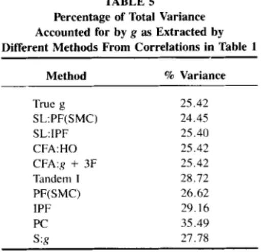
the iterated first principal factor (IPF), and Spearman’s g (S:g), overestimate or underestimate the true percentage of the total variance accounted for by g? The answer is shown in Table 5. The overall root mean square error (RMSE) of the estimated percentages of variance accounted for by g is 3.91%. (Because the PC always includes some of the uniqueness of each variable, it necessarily overestimates x; if we omit PC, the overall RMSE = 2.13s.)

Agreement Between Various Methods Applied to Empirical Data

In a correlation matrix based on empirical data, it is of course impossible to know exactly the true g loadings of the variables. However, we can examine the degree of consistency of the g vector obtained by different methods of factor analysis when they are applied to the same data. For this purpose, we have used a classic

TABLE 5 Percentage of Total Variance Accounted for by g as Extracted by Different Methods From Correlations in Table 1

Method % Variance True g 25.42 SL:PF(SMC) 24.45 SL:IPF 25.40 CFA:HO 25.42 CFA:g + 3F 25.42 Tandem I 28.72 PF(SMC) 26.62 IPF 29.16 PC 35.49 s:g 27.78

(21)

WHAT IS A GOOD R’? 2.51

set of mental test data, originally collected by Holzinger and Swineford ( 1939) consisting of 24 tests given to 145 seventh- and eighth-grade students in a suburb of Chicago. Descriptions of the 24 tests and a table of their intercorrelations (to three decimal places) are also presented by Harman (1976, pp. 123-124). The tests are highly diverse and comprise four or five mental ability factors besides g: spatial relations, verbal, perceptual speed, recognition memory, and associative memory. But certain analyses reveal only one memory factor comprising both recognition and association.

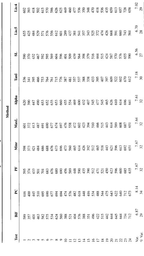
This 24 X 24 R-matrix has been factor analyzed by IO methods. The g loadings of the 24 tests obtained by each method are shown in Table 6. These methods and their abbreviations in Table 6 are: Holzinger’s bi-factor analysis (BiF); principal components (PC); principal factors (PF); “minres” or minimized residu- als (Minr); maximum likelihood (MaxL); Alpha factor analysis (Kaiser & Caf- frey, 1965); Comrey’s Tandem I (Tam) factor analysis (Comrey, 1967, 1973; Comrey & Lee, 1992); Schmid-Leiman (1957) orthogonalized hierarchical analysis (SL); and two applications of LISREL, in each of which Model C (Figure 5) is specified, first for g + 5 factors (LIS:5), then for g + 4 factors (LlS:4). The hypothesis of four group factors gives an overall better fit to the data than five group factors.4

The percentage of total variance in the 24 tests accounted for by g differs across the various methods, ranging from 27% (for the Schmid-Leiman hierarchical g) to 34% (for the first principal component), with an overall average of 30.4% (SD = 2.1%). In short, the various methods differ very little in the percentage of variance accounted for by g.

How similar are the g vectors across different methods‘? Table 7 shows the Pearson correlations and the congruence coefficients of the g vectors. The figures speak for themselves. The first principal component of the correlations shown in the upper triangle of Table 7 accounts for 92.4% of the total variance in this correlation matrix. The mean correlation is ,916; the mean congruence coefficient is .995. They determine also how closely the g vectors resemble one another in the rank order of their g loadings. Spearman’s rank-order correlation (rho) was computed between all the vectors, and it ranges from ,792 to ,995, with an overall mean of ,909.

Wilks’s Theorem and g Factor Scores

If a researcher’s only purpose in factor analyzing a battery of tests is to obtain people’s g factor scores, the method of obtaining g is of little consequence and rapidly decreases in importance as the number of tests in the battery increases. An individual’s g factor scores are merely a weighted average (i.e., linear com-

4The 8 + 5 factors solution has a goodness-of-fit index of .845 (on a scale from 0 to 1) and the root mean square error (RMSE) is .063; the R + 4 factors solution has a GFI of ,884 and an RMSE of ,046.

(22)

TABLE 6 g Factor Loadings on 24 Tests Obtained by 10 Methods Method Test BiF PC PF Minr MaxL Alpha Tan1 SL Lid I 5x9 2 357 3 401 4 463 5 582 6 575 1 s34 8 624 9 560 10 388 I1 521 12 404 13 516 14 388 15 351 16 496 17 422 18 515 19 442 20 644 21 645 22 644 23 134 24 712 Var. 6.87 vi Var. 29 616 595 598 601 620 536 590 655 602 400 374 313 312 390 341 370 425 445 433 421 413 447 395 432 484 418 510 501 484 487 490 466 467 529 695 701 686 691 653 153 592 571 690 683 688 690 652 164 595 576 617 616 616 617 635 761 569 556 694 680 613 614 653 715 604 612 694 690 696 691 660 716 596 601 414 456 473 416 455 387 401 289 516 589 560 558 554 481 509 437 482 448 465 412 469 357 439 381 618 590 614 602 600 537 564 541 448 435 426 423 432 388 398 351 416 390 392 394 407 338 319 343 534 512 512 510 545 433 516 525 488 471 465 466 411 395 444 312 544 521 518 51s 545 407 515 474 475 450 443 443 465 397 424 426 643 623 621 614 626 609 587 668 622 596 596 589 610 522 570 591 640 600 613 608 614 602 576 660 712 685 692 687 696 670 655 743 613 635 651 651 641 612 590 561 8.14 1.67 1.61 1.64 7.61 7.18 6.56 6.70 34 32 32 32 32 30 27 28 Note. Decimals omitted

(23)

TABLE 7

Correlations (Above Diagonal) and Congruence Coefficients (Below Diagonal) Between g Loadings of 24 Tests Extracted by 10 Methods

Method

BiF PC PF Minr MaxL Alpha Tan1 SL Lis:.5 Lis:4

BiF 906 865 876 865 928 145 945 881 945 PC 996 993 997 995 992 940 914 825 919 PF 995 1000 993 993 980 954 955 794 881 Minr 995 1000 1000 999 985 949 960 794 899 MaxL 995 1000 1000 1000 981 952 954 782 895 Alpha 997 1000 999 999 999 905 992 859 932 Tan1 984 992 994 994 994 990 866 747 805 SL 991 999 998 999 998 1000 988 900 940 Lis: I 995 992 991 991 991 993 984 995 897 Lis:F 998 997 996 996 996 997 987 997 995

Note. Decimals omitted.

posite) of his or her standardized scores (e.g., z) on the various tests. A theorem put forth by Wilks (1938) offers a mathematical proof that the correlation between two linear composites having different sets of (all positive) weights tends toward one as the number of positively intercorrelated elements in the composite increases. These conditions are generally met in the case of g factor scores, and with as many as 10 or more tests in the composite, the particular weights will make little difference. For instance, the R factor scores of the normative sample of 9,173 men and women (ages 18 to 23) were obtained from the 10 diverse tests of the Armed Services Vocational Aptitude Battery (ASVAB) when they were factor analyzed by 14 different methods (Ree & Earles, 1992). The average correlation obtained between g factor scores based on the different methods of factor analysis was .984, and the average of all the x factor scores was correlated ,991 with a unit-weighted composite of the 10 ASVAB test scores.

SUMMARY AND CONCLUSIONS

We have been concerned here, not with the nature of K, but with the identijka- tion of g in sets of mental tests, that is, with the relative degree to which each of the various tests in the set measures the one source of variance common to all of the tests, whatever its nature in psychological or physiological terms. Various methods have been devised for identifying g in this psychometric sense. And what we find, both for simulated and for empirical correlation matrices, is that, when a general factor is indicated by all-positive correlations among the variables, the estimated g factor is remarkably stable across different methods of factor analysis, so long as the method itself does not artificially preclude the

(24)

estimation of a general factor. This high degree of stability of g, in terms of correlation and congruence coefficients, refers both to the vector of g loadings of the variables and to the g factor scores of individuals. There is also a high degree of agreement among methods (with the exception of principal components) in the percentage of the total variance in test scores that is accounted for by g.

In fact, the very robustness of g to variations in method of extraction makes the recommendation of any particular method more problematic than if any one method stood out by every criterion as clearly superior to all the others. Because apparently no one method yields a g that is markedly and consistently different from the g of rival methods, how best can we estimate a good g? It is reassuring, at least, that one will probably not go far wrong with any of the more commonly used methods, provided, of course, reasonable attention is paid to both statistical and psychometric sampling. An important implication of this conclusion is that, whatever variation exists among the myriad estimates of g throughout the entire history of factor analysis, exceedingly little of it can be attributed to differences in factor models or methods of factoring correlation matrices.

Recognizing that in empirical science R can be only estimated, the notion of a good g has two possible meanings: (1) an estimated g that comes very close to the unknown true g, in the strictly descriptive or psychometric sense (as in our simulated example), and (2) an estimated g that is more “interesting” than some other estimates of g by virtue of the strength of its relation to other variables (causes and effects of R) that are independent of the psychometric and factor analytic machinery used to estimate g, such as genetic, anatomical, physiological, nutri- tional, and psychological-educational-social-cultural variables-in other words, the “g beyond factor analysis” (Jensen, 1987a). It is in the second sense, obviously, that g is of greatest scientific interest and practical importance. Factor analysis would have little value in research on the nature of abilities if the discovered factors did not correspond to real elements or processes, that is, unless they had some reality beyond the mathematical manipulations that derived them from a correlation matrix. But advancement of our scientific, or cause-and-effect, un- derstanding of g would be facilitated initially by working with a good g in the first sense. This would be a feedback loop, such that cause-and-effect relations of extrapsychometric variables to initial estimates of R would influence subsequent estimates and methods for estimating g, which could then lead to widening the network of possible connections between g and other cause-and-effect variables. Suggested Strategy for Extracting a Good g

Assuming at the outset a correlation matrix based on a subject sample of ade- quate size and on reasonable psychometric sampling of the mental abilities domain, both in the number and variety of tests, the procedure we suggest for estimating g calls for the following steps:

1. Be sure that all variables entered into the analysis are experimentally independent; that is, no variables in the matrix should constitute merely different