國 立 交 通 大 學
顯 示 科 技 研 究 所
碩士論文
非同步鎖模摻鉺光纖雷射參數可調特性之
研究
Tuning characteristics of asynchronous
mode-locked Er-doped fiber lasers
研究生 : 黃耀德
指導教授 : 賴暎杰 博士
非同步鎖模摻鉺光纖雷射參數可調特性之
研究
Tuning characteristics of asynchronous
mode-locked Er-doped fiber lasers
研 究 生:黃耀德 Student:Yao-de Huang
指導教授:賴暎杰 Advisor:
Yinchieh Lai
國立交通大學 電機學院 顯示科技研究所
碩 士 論 文
A Thesis
Submitted in partial Fulfillment of the Requirements for the Degree of Master in
The Department of Photonics and The Institute of Display College of Electrical Engineering
National Chiao Tung University
June 2013 Hsinchu, Taiwan, Republic of China
非同步鎖模摻鉺光纖雷射參數可調特性之
研究
研究生:黃耀德 教授:賴暎杰 博士
國立交通大學顯示科技研究所
摘要
本論文主要研討非同步鎖模摻鉺光纖雷射之參數可調特性。在混 合式主被動諧波鎖模機制的雷射實驗架構中﹐藉由雷射參數的改變, 以 RF 頻譜分析儀上所獲得的數據為主,OSA 光譜分析儀上所獲得的 資訊為輔,來深入了解同步/非同步鎖模轉換與調變強度、調變頻率 等雷射參數之間的關係,另一方面也利用變分推導與數值分析的方式 來模擬同步區間到非同步區間的過渡變化。 在實際實驗上,雷射相位調變器的操作頻率為 10GHz 與 20GHz, 我們在此二頻率附近來作調變頻率之改變以及調變強度之改變,觀察 的重點主要是諧頻的變化以及同步/非同步區間邊界的雷射操作狀 態。透過光譜與頻譜分析儀之量測結果,我們發現 10GHz 和 20GHz 的操作態有稍微不同之雷射特性呈現。經由實驗的結果,我們驗證了 同步/非同步鎖模區間之轉換邊界與雷射參數的關係,並能與基於變 分法的理論結果來作比較。Tuning characteristics of asynchronous
mode-locked Er-doped fiber lasers
Student:Yao-de Huang Advisor:Dr. Yinchieh Lai
Department of Photonics and The Institute of Display
College of Electrical Engineering
National Chiao Tung University
Abstract
The thesis is focused on the study of the tuning characteristics for asynchronous mode-locked Er-doped fiber lasers. With the experimental laser structure of hybrid active/passive mode-locking, laser performance data under parameter tuning are collected by the RF spectrum and optical spectrum analyzer to understand the relationship among the
synchronous/asynchronous mode-locking and the modulation
intensity/frequency. We also use the variational method and numerical solution to study the transition between the synchronization and non-synchronization operation states.
In the experiment, the phase modulator is operated with the modulation frequency around the 10GHz and 20GHz with different modulation strengths. The changes of the RF spectra and the transition from synchronization to non-synchronization are the main focuses of observation. The 10GHz and 20GHz operation states exhibit slightly different performance characteristics. We experimentally verify the synchronous/asynchronous laser transition properties and compare the experimental observations with the theoretical predictions based on the variational method.
誌謝
碩士班兩年的時間也即將接近尾聲了,在最後完成碩士論文的這 段時間內更是受到許多貴人的相助。 首先要感謝的是我的碩士班指導教授賴暎杰老師,每當和賴老師 討論實驗或者是理論時,總會覺得那段時間是很愉快的。有時候遇到 了難題,到了老師面前總是迎刃而解,同時老師也讓我能更有效率並 且正確的完成實驗。在賴老師面前,彷彿所有問題都能夠輕而易舉的 解決,也希望自己在未來,處理問題方面能像賴老師一樣。 感謝實驗室鞠曉山學長、吳尚穎學長、王聖閔學長、許宜蘘學姊 以及實驗室助理黃淑惠小姐,在我的課業或日常瑣事上的指導。同時 也要謝謝實驗室的夥伴們,江國豪、楊良愉、林仕斌、王一評、羅丞 志、顏光廷、周彥旭,讓我在學習的路上並不是孤單一人。 另外要特別感謝的是交大管弦樂社以及管樂社,能夠在我碩班兩 年時參與,在平常課餘時間,能夠在社團中找尋到除了課業以外我想 追尋的東西。 最後也要謝謝我的家人,感謝你們在我的求學階段,不用為了課 業以外的事物煩惱,讓我沒有後顧之憂。Contents
Chinese Abstract……….………… I English Abstract………...………. II Acknowledgement………..………. III Contents……….…………..IV List of Figures………..VI Chapter 1 : Introduction 1.1 Overview………...…….1 1.2 Motivation………..………4 1.3 Organization………..…………5 References………...6Chapter 2 : Principles of mode-locked fiber lasers 2.1 Synchronously active mode-locking………..……7
2.1.1 Phase modulation mode-locking………..……8
2.1.2 Amplitude modulation mode-locking……….…...10
2.2 Asynchronously mode-locked fiber lasers………...…13
2.3 Master equation for asynchronously mode-locked fiber Lasers………..…………16 2.4 Solution of the master equation by the variational
method………..17
References……….….…….19
Chapter 3: Experimental setup and results 3.1 Experimental setup………..…………22
3.2 Parameter tuning………..………25
3.2.1 10 GHz operation………..….25
3.2.2 20 GHz operation………..…….34
3.3 Comparison and discussion……….36
References……….…..53
Chapter 4: Conclusions 4.1 Summary of achievements………...…54
List of Figures
Fig 1.1 Relationship between Synchronous/asynchronous and detuning frequency………4 Fig. 2.1 Schematic of an active mode-locked laser………7 Fig. 2.2 Actively mode-locked pulses in the time domain and the time dependence of the net gain………...10 Fig. 2.3 Actively mode-locked modes in the frequency domain……...11 Fig. 2.4 Sketch of the amplitude modulation mode-locking in the
frequency domain……….12 Fig. 2.5 Laser cavity with the gain, filter, (group velocity dispersion) GVD, (self phase modulation) SPM and the phase modulation driven asynchronously……….14 Fig.2.6 The noise-cleanup effect in the asynchronous soliton mode-locked laser………...15 Fig. 3.1 Experimental setup………..22
Fig. 3.2 Change of the modulation frequency………...25
Fig. 3.3 Schematic diagram for modulation frequency and cavity
frequency ……….26 Fig. 3.4 RF spectrum of the laser output near 10GHz with 1MHz
span………..26 Fig. 3.5 Optical spectrum of the laser output near 1560nm with 20nm span………..26 Fig. 3.6 Schematic diagram for modulation frequency and cavity
frequency ………27 Fig. 3.7 RF spectrum of the laser output near 10GHz with 1MHz
span………..27 Fig. 3.8 Optical spectrum of the laser output near 1560nm with 20nm span………..27 Fig. 3.9 Schematic diagram for modulation frequency and cavity
frequency ………28 Fig. 3.10 RF spectrum of the laser output near 10GHz with 1MHz
span………..……28 Fig. 3.11 Optical spectrum of the laser output near 1560nm with 20nm span………...28 Fig. 3.12 Schematic diagram for modulation frequency and cavity
frequency ……….29 Fig. 3.13 RF spectrum of the laser output near 10GHz with 1MHz
Fig. 3.14 Optical spectrum of the laser output near 1560nm with 20nm span………...29 Fig. 3.15 Schematic diagram for modulation frequency and cavity
frequency ……….30 Fig. 3.16 RF spectrum of the laser output near 10GHz with 1MHz
span………...30 Fig. 3.17 Optical spectrum of the laser output near 1560nm with 20nm span………...30 Fig. 3.18 Schematic diagram for modulation frequency and cavity
frequency ……….31 Fig. 3.19 RF spectrum of the laser output near 10GHz with 1MHz
span………...31 Fig. 3.20 Optical spectrum of the laser output near 1560nm with 20nm span………...31 Fig. 3.21 Repetition frequency versus modulation frequency at
10GHz,-5dBm………..32 Fig. 3.22 Repetition frequency versus modulation frequency at
10GHz,-6dBm………...………33 Fig. 3.23 Repetition frequency versus modulation frequency at
10GHz,-8dBm………...……33 Fig. 3.24 Repetition frequency versus modulation frequency at
20GHz,-5dBm………...…34 Fig. 3.25 Repetition frequency versus modulation frequency at
20GHz,-6.5dBm………....35 Fig. 3.26 Repetition frequency versus modulation frequency at
20GHz,-8dBm………...35
Fig. 3.27 Originally defined modulation frequency and harmonic
frequencies ……….36
Fig. 3.28 Defined modulation frequency versus pulse repetition
frequency ……….37
Fig. 3.29 Detuning frequency versus the pulling frequency ,at
10GHz,-5dBm………...39
Fig. 3.30 Detuning frequency versus the pulling frequency ,at
20GHz,-5dBm………..……39
Fig. 3.31 Detuning frequency versus the pulling frequency ,at
10GHz,-6.5dBm………40
Fig. 3.32 Detuning frequency versus the pulling frequency ,at
Fig. 3.33 Detuning frequency versus the pulling frequency ,at
10GHz,-8dBm………..41
Fig. 3.34 Detuning frequency versus the pulling frequency ,at
20GHz,-8dBm………...41 Fig. 3.35 Simulation results for synchronous/asynchronous
transition………...42 Fig 3.36 Synchronous/asynchronous transition points under different modulation strengths………...……….45 Fig. 3.37 Synchronous/Asynchronous transition points under theoretical results………...……….46
Fig. 3.38 Detuning frequency versus asynchronous mode-locking
deviation frequency ,at 10GHz,-5dBm………....47
Fig. 3.39 Detuning frequency versus asynchronous mode-locking
deviation frequency ,at 20GHz,-5dBm………....47
Fig. 3.40 Detuning frequency versus asynchronous mode-locking
deviation frequency ,at 10GHz,-6.5dBm………...48
Fig. 3.41 Detuning frequency versus asynchronous mode-locking
deviation frequency ,at 20GHz,-6.5dBm………...…..48
deviation frequency ,at 10GHz,-8dBm………....49
Fig. 3.43 Detuning frequency versus asynchronous mode-locking
deviation frequency ,at 20GHz,-8dBm………..…..49
Fig. 3.44Transition points when the asynchronous mode-locking
disappear...………...……….51 Fig. 3.45 RF spectrum of the laser output with large deviation
frequency. ………..……..52 Fig. 3.46 Optical spectrum of the laser output with bound
pulses. ………..……52
List of Tables
Table 3.1 Devices in the fiber ring cavity……….……24 Table 3.2 Synchronous/asynchronous transition points under different modulation strengths.………...…45 Table 3.3 Synchronous/Asynchronous transition points under theoretical results.………...………46 Table 3.4 Transition points when the asynchronous mode-locking
Chapter 1
Introduction
1.1 Overview
Fiber laser is a laser with a doped fiber as the gain medium, or just a laser with a laser cavity where most of the laser resonator is made of fibers. The fiber gain medium is a fiber typically doped with rare earth
ions such as erbium (1550nm) or ytterbium (1060nm). One or
several fiber-coupled laser diodes are used for pumping. The 1550nm wavelength region has been widely utilized as the fiber communication spectral window, simply because the 1550nm wavelength region has the lowest fiber propagation loss. In contrat, the ytterbium-doped gain media is often used for high-power lasers and for wavelength-tunable solid-state lasers, mainly because the ytterbium-doped fiber laser is with very high efficiency. The rapid progress was also driven by a correspondingly impressive development of low-cost, high-brightness, fiber-coupled pump diodes as the pump sources, enabling development of compact systems with extremely high efficiency.
Fiber lasers has many types, such as Q-switched fiber lasers, high-power fiber lasers, upconversion fiber lasers, narrow-linewidth fiber
lasers, mode-locked fiber lasers, etc. Q-switching, sometimes known as giant pulse formation, is a technique by which a laser can be made to produce a pulsed output beam [1.1]. Q-switched lasers are based on the modulation of the optical cavity’s quality factor. In comparison to mode-locking, Q-switching typically leads to much lower pulse repetition rates, much higher pulse energies, and much longer pulse durations.
High-power fiber lasers are mostly based on double-clad fibers [1.2]. The gain medium forms the core of the fiber, which is surrounded by two layers of cladding. The lasing mode propagates in the core, while a multimode pump beam propagates in the inner cladding layer. The outer cladding keeps this pump light confined. This arrangement allows the core to be pumped with a much higher-power beam than could otherwise be made to propagate in it, and allows the conversion of the pump light with relatively low brightness into a much higher-brightness signal.
There are two general ways to achieve mode-locking: one is the passive mode-locking and the other is the active mode-locking. Typically the passive mode-locking can generate shorter pulses than active mode-locking. On the other hand, the active mode-locking can generate
higher repetition rates than passive mode-locking. Passive mode-locking can be implemented by a variety of different mechanisms, such as
saturable absorber mode-locking, polarization additive-pulse
mode-locking (P-APM) and stretched-pulse additive-pulse mode-locking. In contrast, active mode-locking can use two different methods of optical modulation: amplitude modulation (AM) mode-locking and phase modulation mode-locking. One of the major advantages of active mode-locking is that it allows synchronized operation of the mode-locked laser to an external radio frequency (RF) source. This is very useful for optical fiber communication, where synchronization is normally required between optical signal and electronic control signal. In addition, there are also hybrid active/passive mode-locked lasers. One example is the asynchronous mode-locked Er-doped fiber soliton laser which has been developed in our lab over the past years. Theoretical analyses based on the master equation model solved by the variational method have been carried out. All the pulse parameters of the laser output will exhibit complicated slow periodic variations under the asynchronous soliton mode-locking mode [1.3][1.4]. This is also the mode-locked fiber laser system that will be investigated in this thesis study.
1.2 Motivation
Asynchronous mode-locking is a hybrid active/passive laser mode-locking mechanism in which the frequency of intracavity phase modulation is slightly detuned away from the cavity harmonic repetition frequency by a few tens of kilohertz. In this thesis study, we want to investigate the synchronous/asynchronous transition properties, and in particular, how the transition is affected by the laser parameters. The changes of the RF spectra under the transition from synchronization to non-synchronization are the main focuses of observation. These experimental observations can then be compared with the theoretical modeling to help understand more deeply the laser dynamics of asynchronous mode-locking.
Fig 1.1 Relationship between Synchronous/asynchronous and detuning frequency.
1.3 Organization
The thesis consists of four chapters. Chapter 1 is an overview and describes the motivation for doing this research. Chapter 2 describes the methods of different mode-locking techniques and the solution of the mode-locked laser master equation by the variational method. Chapter 3 describes the experimental setup and results. Finally Chapter 4 presents the summary and possible future work.
Reference
[1.1] J. Lee, J. Koo, Y. M. Chang, P. Debnath, Y.W. Song, and J. H.
Lee,” Experimental investigation on a Q-switched, mode-locked
fiber laser based on the combination of active mode locking and passive Q switching” J. Opt. Soc. Am. B. 6 ,1479 (2012).
[1.2] I. Pavlov, E. Ilbey, E. Dülgergil, A. Bayri, and F. Ö . Ilday, “High-power high-repetition-rate single-mode Er- Yb-doped fiber laser system” Optics Express, 9, 9471 (2012).
[1.3] W. W. Hsiang, H. C. Chang, and Y. Lai, “Laser dynamics of a 10
GHz 0.55 ps asynchronously harmonic modelocked Er-doped fiber soliton Laser”, IEEE J. Quantum Electron. 3, 292 (2010).
[1.4] H. A. Haus, “Mode-locking of lasers,” IEEE J. Quantum
Chapter 2
Principles of mode-locked fiber lasers
2.1 Synchronously active mode-locking
The active mode-locking is achieved by modulating the loss or phase of the laser cavity. When the modulation frequency is synchronized with the cavity’s round trip time, the pulse train in the resonator will continue to grow and then achieve stable mode-locking. Generally, active modulation can be achieved with an acousto-optic or electro-optic modulator.
As explained above, active mode-locked fiber lasers can use two different methods for optical modulation. The two different methods will be given in the following two sub-sections (2.1.1 and 2.1.2). One is the amplitude modulation mode-locking (AM) and the other is the phase modulation mode-locking.
2.1.1 Phase modulation mode-locking
A phase modulator is an optical modulator which can be used to control the optical phase of a laser beam. By modulating the phase of the optical field in the laser cavity periodically, it can achieve mode-locking without changing the amplitude of the optical field and then produce
short pulse trains.This mechanism can be analyzed both in the frequency
domain and the time domain [2.1].
In the time domain, the phase modulator provides a phase change for the optical pulse. Assume the pulsewidth is much smaller than the modulation period, then the optical phase changed by the phase modulator can be expressed as,
d d t t t dt dt 2 2 0 2 ( ) (2.1)
This term0 is only a constant phase that has no effect on optical pulses. When the optical pulse passes through the modulator, the central
frequency of the pulse will shift if d 0
dt . ( d dt is the immediate frequency). The central frequency of the optical pulse will continue to shift by modulation until this pulse is shifted outside of the gain
bandwidth and disappears. Therefore, only at d 0
dt
the pulse can
shifted by modulation.
Actually, d 0
dt
have two solution states, but in most situations only one state can be stable and the other can’t. Which solution state can exist in the cavity depends on the sign of the cavity dispersion. This is because the second order term
2 2
d dt
provides a chirp to the pulse and will affect the optical propagation of the pulse by interacting with the dispersion.
In the frequency domain, let us assume ω0 is the angular frequency of
the longitudinal mode. When this mode passes through the phase modulator, the optical signal can be written below:
(2.2)
where M is the modulation index, is the modulation frequency.
It can be expanded as:
(2.3),
is the n-th order Bessel function. From the formula it can be observed that the optical signal consist of unlimited sidebands. These sidebands can phase-lock adjacent modes through injection locking and then the periodic pulse train will be formed.
2.1.2 Amplitude modulation mode-locking
Amplitude modulation mode-locking is a method to produce a short pulse train by modulating the optical amplitude of the light. It also can be analyzed both in the time domain and frequency domain.
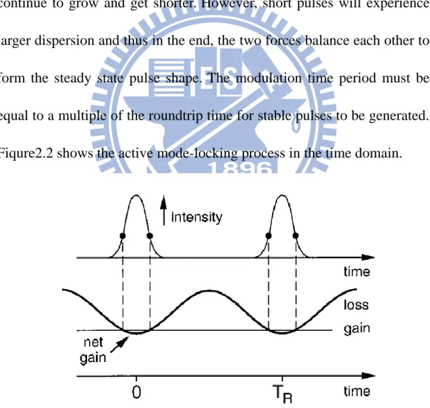
In the time domain, the modulation provides a time dependent loss. When the gain is greater than the loss, the optical pulse trains will continue to grow and get shorter. However, short pulses will experience larger dispersion and thus in the end, the two forces balance each other to form the steady state pulse shape. The modulation time period must be equal to a multiple of the roundtrip time for stable pulses to be generated. Fiqure2.2 shows the active mode-locking process in the time domain.
In the frequency domain, as the gain level is above threshold, the net gain of the system is greater than zero, then the longitudinal modes will begin to lase. The longitudinal modes are separated equally in frequency
domain and the frequency interval is , where is the round
trip time. Again these sidebands will injection-lock the neighboring modes sequentially and the mode-locking is formed eventually. Figure 2.3 shows the active mode-locking process in the frequency domain.
If the central mode without amplitude modulation is expressed as E0
cos(ω0t), then the amplitude modulated optical signal can be expressed as:
0
1+ cos
Mcos
0E t( ) E
(
M
t
)
(
t
)
0
cos
0+
0cos
0+
0cos
0+
2
M2
ME
(
t
)
EM
(
)
t
EM
(
)
t
(2.5)We denoted the modulation depth is M and the modulation frequency is .
The central frequency ωo produces two sidebands (ω0±ΩM) which
have the same phase after the modulation. When these modes pass
through the amplitude modulator again, the other two inphase sidebands (ω0±2ΩM) will be produced. This process will repeat until all the
longitudinal modes in the gain bandwidth are locked. Due to mode-locking, these frequency components that are separated ΩM will
have fixed phase relation and will produce a periodical pulse train in the time domain.
2.2 Asynchronously mode-locked fiber lasers
In normal active harmonic mode-locked lasers, the optical modulator is driven synchronously with respect to the cavity harmonic frequency. The optical pulses will be shifted by a frequency if not synchronized. With the finite bandwidth filter and gain, the pulse trains cannot achieve stable mode-locking. However, in the asynchronous soliton mode-locked laser [2.2], the modulation frequency and the cavity harmonic frequency have a small deviation frequency from several kHz to tens kHz and stable mode-locking still can be achieved [2.3] .
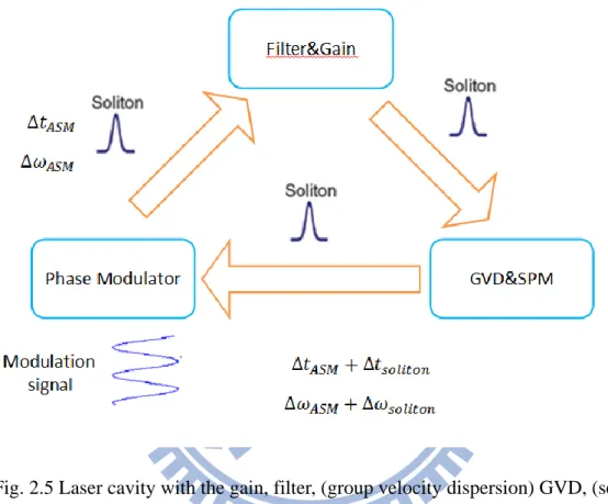
The fiber laser is consisted of the gain, the optical bandpass filter, group velocity (GVD), self phase modulation (SPM) and the phase
modulator driven asynchronously. Because of asynchronous modulation,
the optical pulses reach the optical modulator not always at the peaks of the modulation signal. When the pulse passes through the phase modulator, the central wavelength of the pulse can get a small frequency shift. When the nonlinear effects are not considered, the asynchronous modulation will shift the central frequency of the pulses periodically with accumulation. The gain medium and the filter are both fixed with finite
bandwidth, the overdeveloped amount of central frequency shift can make the pulse leave the center of the gain or the filter. Then the pulses can’t exist in the cavity since they will experience quite large loss.
Fig. 2.5 Laser cavity with the gain, filter, (group velocity dispersion) GVD, (self phase modulation) SPM and the phase modulation driven asynchronously.
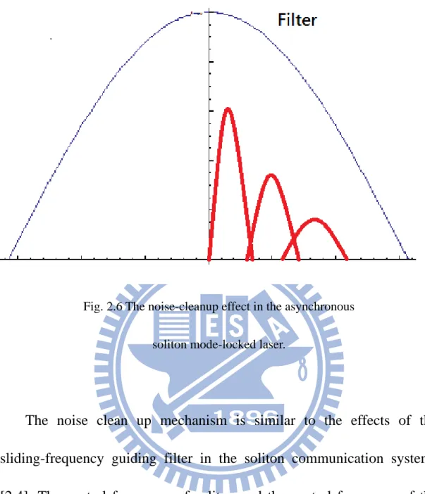
Fig. 2.6 The noise-cleanup effect in the asynchronous soliton mode-locked laser.
The noise clean up mechanism is similar to the effects of the sliding-frequency guiding filter in the soliton communication systems [2.4]. The central frequency of soliton and the central frequency of the filters will vary together in the fiber cavity during propagation, but the central frequency of the linear noise keeps fixed and will be filtered out by the optical filter. So a higher SMSR (Side Mode suppression ratio) can be obtained [2.5], even when there is no explicit intracavity optical device to suppress the supermode noises.
2.3 Master equation for asynchronously mode-locked fiber Lasers
The master equation model for asynchronous mode-locked lasers is given as [2.1][2.3][2.6][2.7]:
The equation is derived under the assumption of small round-trip change.
Here is the complex field envelope of the pulse, is the
number of the cavity round trip time, is time, is linear gain, is
saturation energy, is linear loss, is the effect of the optical filtering, is group velocity dispersion, is the effect of equivalent fast
saturable absorber, is the self-phase modulation coefficient, is the
phase modulation depth, is the modulation frequency, and is the
timing walk-off per round trip.
is the deviation frequency between the N-th cavity harmonic
frequency and the modulation frequency . In analyses, the
sinusoidal modulation curve of the phase modulator can be expanded by Taylor’s series as:
where
.
2.4 Solution of the master equation by the variational method
The master equation can be solved approximately by using the variational method developed in [2.7]. By assuming the following solution ansatz :
where is the optical center frequency, is timing, is
chirp, is the amplitude, and is the pulserwidth, one can
These ordinary differential equations can then be solved numerically to study the laser dynamics of asynchronous mode-locking.
Reference
[2.1] H. A. Haus, “Mode-locking of lasers,” IEEE J. Quantum
Electron. 6, 1173 (2000).
[2.2] C. R. Doerr, H. A. Haus, and E. P. Ippen, “Asychronous soliton
mode locking”, Opt. Lett. 19, 1958 (1994).
[2.3] H. A. Haus, D. J. Jones, E. P. Ippen, and W. S. Wong, “Theory of
soliton stability in asynchronous modelocking,” IEEE J. Lightwave Technol. 14, 622 (1996).
[2.4] L. F. Mollenauer, J. P. Gordon, and S. G. Evangelides, ‘‘The sliding frequency guiding filter: an improved form of soliton jitter control,’’ Opt. Lett. 17, 1575 (1992).
[2.5] G. T. Harvey and L. F. Mollenauer, “Harmonically mode-locked
fiber ring laser with an internal Fabry-Perot stabilizer for soliton transmission,” Opt. Lett. 2, 107 (1993)
[2.6] H. A. Haus, J. G. Fujimoto, and E. P. Ippen, “Structures for additive pulse mode locking,” J. Opt. Soc. Amer. B, vol. 8, pp. 2068–2076, 1991.
[2.7] W. W. Hsiang, H. C. Chang, and Y. Lai, “Laser dynamics of a 10
soliton Laser”, IEEE J. Quantum Electron. 3, 292 (2010).
[2.8] W. W. Hsiang, C. Y. Lin, M. F. Tien, and Y. Lai, “Direct
generation of a 10 GHz 816 fs pulse train from an erbium-fiber soliton laser with asynchronous phase modulation,” Opt. Lett. 30, 2493 (2005).
[2.9] W. W. Hsiang, C. Lin, N. Sooi, and Y. Lai, “Long-term
stabilization of a 10 GHz 0.8 ps asynchronously mode-locked Er-fiber soliton laser by deviation-frequency locking,” Opt. Exp. 5, 1822 (2006).
[2.10] M. C. Chan, “Hybrid Mode-locking Er-doped Fiber Laser,” Institute of Electro-Optical engineering in National Chiao-Tung University, master thesis (2002).
[2.11] M. Nakazawa and M. Yoshida, “Scheme for independently stabilizing the repetition rate and optical frequency of a laser using a regenerative mode-locking technique”, Opt. Lett. 33, 1059 (2008). [2.12] H. G. Weber and M. Nakazawa, “Ultrahigh-Speed Optical
Transmission Technology” ,(2007).
[2.13] B. E. A. Saleh and M. C. Teich , Fundamentals of Photonics , Wiley-Interscience, Canada, (2007).
[2.14] D. J. KUIZENGA, and A .E. SIEGMAN “FM and AM mode locking of the homogeneous laser,” IEEE J. Quantum Electron. 6, 694 (1970).
[2.15] M. Nakazawa, K. Kasai, and M. Yoshida,” C2h2 absolutely
optical frequency-stabilized and 40 GHz repetition rate stabilized regeneratively mode-locked picosecond erbium fiber laser at 1.53 μm” Opt. Lett. 33, 2641(2008).
Chapter 3
Experimental setup and results
3.1 Experimental setup
The system setup of our asynchronous mode-locked Er-doped fiber lasers is shown in Fig 3.1.
Fig. 3.1 Experimental setup
The Er-doped fiber is pumped by two 980 nm laser diodes. The
isolator in the cavity is for single direction optical wave propagation. There are two couplers used here to distribute optical signal. The coupler
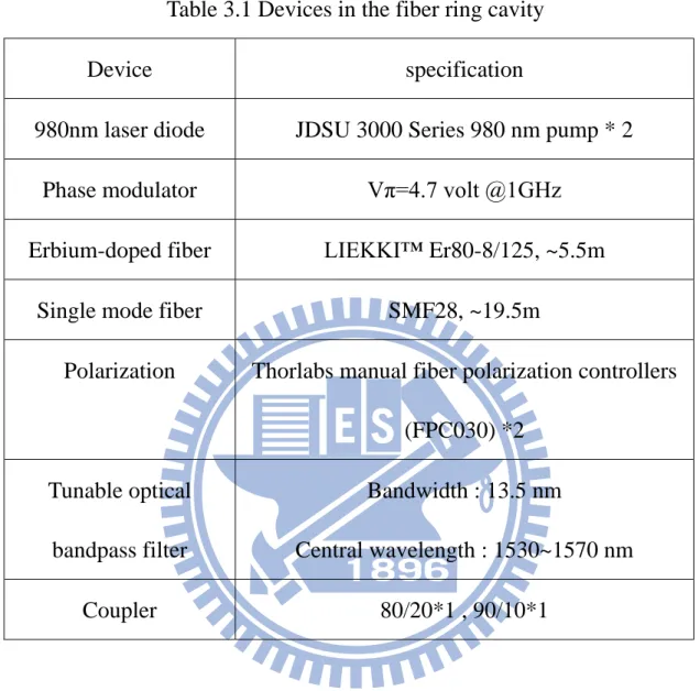
1 divides 80% optical signal into the cavity and 20% into the coupler 2, which divides 10% into the PD. The optical power incident on PD is converted to electrical signals and then into the RF spectrum analyzer. The rest 90% of the optical power is for laser output. The two polarization controllers and the in-line polarizer are used to achieve polarization additive-pulse mode-locking (P-APM). The phase modulator is the core element of the experiment for achieving asynchronous mode-locking. In the experiment we change the modulation frequency and modulation strength to explore the laser dynamics. The devices that have been used in the fiber ring cavity are listed in the Table 3.1
Table 3.1 Devices in the fiber ring cavity
Device specification
980nm laser diode JDSU 3000 Series 980 nm pump * 2
Phase modulator Vπ=4.7 volt @1GHz
Erbium-doped fiber LIEKKI™ Er80-8/125, ~5.5m
Single mode fiber SMF28, ~19.5m
Polarization Thorlabs manual fiber polarization controllers
(FPC030) *2 Tunable optical bandpass filter Bandwidth : 13.5 nm Central wavelength : 1530~1570 nm Coupler 80/20*1 , 90/10*1
3.2 Parameter tuning
3.2.1 10 GHz operation
From Chapter 2, we know how to generate synchronously and
asynchronously mode-locking. The changes of the RF spectra and the transition from synchronization to non-synchronization are the main focuses of observation. We change the modulation frequency and modulation strength to explore the laser dynamics. In the experiment, we first set both the pump lasers at 500 mA. Then we set the phase modulation frequency at 10GHz. With the change of the modulation frequency, we record all the spectral data from the RF spectrum analyzer. The experiment is explained by the schematic diagram in Fig. 3.2 and the measured data are listed afterwards.
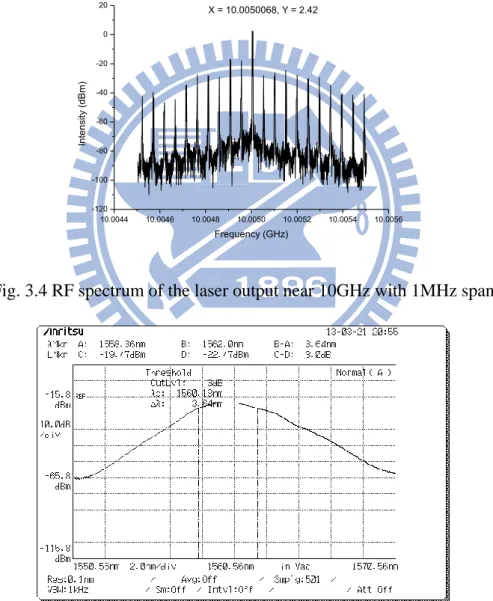
Fig. 3.3 Schematic diagram for modulation frequency and cavity frequency 10.0044 10.0046 10.0048 10.0050 10.0052 10.0054 10.0056 -120 -100 -80 -60 -40 -20 0 20 X = 10.0050068, Y = 2.42 In te nsi ty (d Bm) Frequency (GHz)
Fig. 3.4 RF spectrum of the laser output near 10GHz with 1MHz span
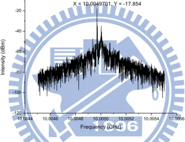
Fig. 3.6 Schematic diagram for modulation frequency and cavity frequency 10.0044 10.0046 10.0048 10.0050 10.0052 10.0054 10.0056 -120 -100 -80 -60 -40 -20 X = 10.0049701, Y = -17.854 In te n si ty (d Bm) Frequency (GHz)
Fig. 3.7 RF spectrum of the laser output near 10GHz with 1MHz span
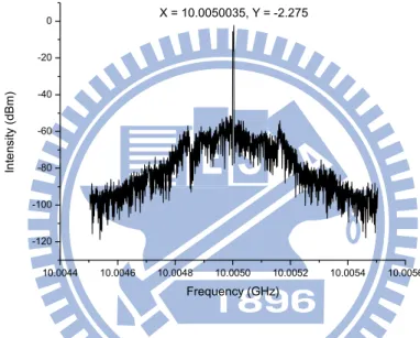
Fig. 3.9 Schematic diagram for modulation frequency and cavity frequency 10.0044 10.0046 10.0048 10.0050 10.0052 10.0054 10.0056 -120 -100 -80 -60 -40 -20 0 X = 10.0050035, Y = -2.275 In te nsi ty (d Bm) Frequency (GHz)
Fig. 3.10 RF spectrum of the laser output near 10GHz with 1MHz span
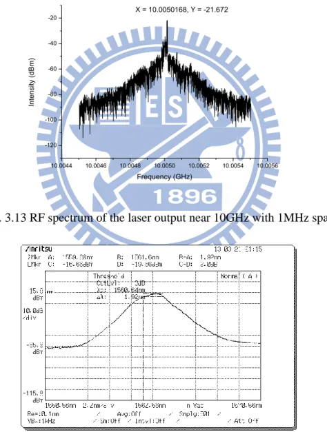
Fig. 3.12 Schematic diagram for modulation frequency and cavity frequency 10.0044 10.0046 10.0048 10.0050 10.0052 10.0054 10.0056 -120 -100 -80 -60 -40 -20 X = 10.0050168, Y = -21.672 In te nsi ty (d Bm) Frequency (GHz)
Fig. 3.13 RF spectrum of the laser output near 10GHz with 1MHz span
Fig. 3.15 Schematic diagram for modulation frequency and cavity frequency 10.0044 10.0046 10.0048 10.0050 10.0052 10.0054 10.0056 -120 -100 -80 -60 -40 -20 0 20 X = 10.0050001, Y = 1.976 In te n si ty (d Bm) Frequency (GHz)
Fig. 3.16 RF spectrum of the laser output near 10GHz with 1MHz span
Fig. 3.18 Schematic diagram for modulation frequency and cavity frequency 10.0044 10.0046 10.0048 10.0050 10.0052 10.0054 10.0056 -120 -100 -80 -60 -40 -20 0 X = 10.0049968, Y = -5.6 In te n si ty (d Bm) Frequency (GHz)
Fig. 3.19 RF spectrum of the laser output near 10GHz with 1MHz span
Fig. 3.20 Optical spectrum of the laser output near 1560nm with 20nm span
for changing the modulation frequency. The data are recorded for each 1 kHz change. Figure 3.4, 3.7, 3.10, 3.13, 3.16, and 3.19 show the measured RF spectra and Figure 3.5, 3.8, 3.11, 3.14, 3.17, and 3.20 show the optical spectra. These experimental data are for the case of 10G Hz, -5dBm.
From the stored RF spectra, we can also read the repetition frequencies and plot them below.
10.00496 10.00498 10.00500 10.00502 10.00504 10.00506 10.00508 10.00510 10.00496 10.00497 10.00498 10.00499 10.00500 10.00501 10.00502 10.00503 R e p e tit io n fre q u e n cy (G H z) Modulation frequency (GHz)
10.00488 10.00490 10.00492 10.00494 10.00496 10.00498 10.00500 10.00487 10.00488 10.00489 10.00490 10.00491 10.00492 10.00493 10.00494 R e p e tit io n fre q u e n cy (G H z) Modulation frequency (GHz)
Fig. 3.22 Repetition frequency versus modulation frequency at 10GHz,-6.5dBm
10.00518 10.00520 10.00522 10.00524 10.00526 10.00528 10.00530 10.00532 10.00519 10.00520 10.00521 10.00522 10.00523 10.00524 10.00525 10.00526 R e p e tit io n fre q u e n cy (G H z) Modulation frequency (GHz)
Fig. 3.23 Repetition frequency versus modulation frequency at 10GHz,-8dBm
In figure 3.21, 3.22, and 3.23,the laser repetition frequency versus the modulation frequency for different modulation strength are plotted.
3.2.2 20 GHz operation
To have more data for comparison, we also operate the laser under 20 GHz and record the data as the 10 GHz case. In the following we only show the repetition frequency versus the modulation frequency diagrams.
19.98396 19.98398 19.98400 19.98402 19.98404 19.98406 19.98408 19.98410 19.98396 19.98397 19.98398 19.98399 19.98400 19.98401 19.98402 19.98403 R e p e tit io n fre q u e n cy (G H z) Modulation frequency(GHz)
19.99304 19.99306 19.99308 19.99310 19.99312 19.99314 19.99316 19.99318 19.99304 19.99305 19.99306 19.99307 19.99308 19.99309 19.99310 19.99311 19.99312 R e p e tit io n fre q u e n cy (G H z) Modulation frequency (GHz)
Fig. 3.25 Repetition frequency versus modulation frequency at 20GHz,-6.5dBm
19.98374 19.98376 19.98378 19.98380 19.98382 19.98384 19.98386 19.98388 19.98373 19.98374 19.98375 19.98376 19.98377 19.98378 19.98379 19.98380 19.98381 19.98382 19.98383 R e p e tit io n fre q u e n cy (G H z) Modulation frequency (GHz)
3.3 Comparison and discussion
Before performing the discussion and comparison, we need to introduce some definitions in order to make the following discussion more clear. In figure 3.27, it was commonly believed that the deviation
frequency is simply the difference between the modulation
frequency and the cavity harmonic frequency .However the theory
of the frequency pulling effect predicts that will not be equal to
and the value of will be a function of the modulation depth.
Fig. 3.28 Defined modulation frequency and pulse repetition frequency
In Figure 3.28, we have the modulation frequency , the cavity
harmonic frequency , and the pulse repetition frequency . The
difference between and is the detuning frequency , and the
difference between and is the asynchronous mode-locking
deviation frequency . is the pulling frequency by repetition
frequency pulling effect [3.1].
From figure 3.21, 3.22, 3.23, 3.24, 3.25, and 3.26, one can observe the synchronous to asynchronous transition. We can also calculate the
About the repetition frequency pulling effect, in order to understand the physical meaning of such a linear drift, it is important to note that the master equation model [3.2][3.3] has pre-assumed a fixed laser round trip time. Therefore a constant pulse timing position drift per round trip will correspond to a change of the pulse repetition frequency. Mathematically, the mechanism for producing such a linear drift is as follows. First, all the pulse parameters oscillate sinusoidally due to the sinusoidal excitation of the asynchronous phase modulation, that is, the first term in the right-hand side of Eq. (3.1).
Then, due to the nonlinear characteristics of Eqs. (3.1) and (3.2), small dc components will also appear in the right-hand side of both equations through the nonlinear terms. Finally, the dc components cause the timing to drift linearly since there is no restoring force for the timing position in Eq. (3.2).
-40 -35 -30 -25 -20 -15 -10 -5 0 0 20 40 60 80 100 Detuning frequency (kHz) Pu lli n g fre q u e n cy (kH z)
Fig. 3.29 Detuning frequency and the pulling frequency ,at 10GHz,-5dBm
-40 -35 -30 -25 -20 -15 -10 -5 0 0 20 40 60 80 100 Detuning frequency (kHz) Pu lli n g fre q u e n cy (kH z)
-40 -35 -30 -25 -20 -15 -10 -5 00 10 20 30 40 50 60 70 80 90 100 Detuning frequency (kHz) Pu lli n g fre q u e n cy (kH z)
Fig. 3.31 Detuning frequency and the pulling frequency ,at 10GHz,-6.5dBm
-40 -35 -30 -25 -20 -15 -10 -5 00 20 40 60 80 100 Detuning frequency (kHz) Pu lli n g fre q u e n cy (kH z)
-40 -35 -30 -25 -20 -15 -10 -5 00 10 20 30 40 50 60 70 80 90 100 Detuning frequency (kHz) Pu lli n g fre q u e n cy (kH z)
Fig. 3.33 Detuning frequency and the pulling frequency ,at 10GHz,-8dBm
-40 -30 -20 -10 00 20 40 60 80 100 Detuning frequency (kHz) Pu lli n g fre q u e n cy (kH z)
Fig. 3.34 Detuning frequency and the pulling frequency ,at 20GHz,-8dBm
Figure 3.29, 3.30, 3.31, 3.32, 3.33, and 3.34 are the diagrams of
strengths and frequencies. However, it should be noted that the cavity length drift cannot be ignored if the measurement time is too long. Therefore in the above figures the plotted pulling frequency values may also be offset by the cavity harmonic frequency change due to the cavity length drift.
We have also used the pulse parameter evolution equations in Chapter 2.4 to perform numerical simulation for studying the synchronous-to-asynchronous transition and the calculated results are shown in Fig. 3.35. -40 -35 -30 -25 -20 -15 -10 -5 00 20 40 60 80 100 Detuning frequency fd(kHz) Pu lli n g fre q u e n cy fdelta (kH z)
Here the simulation parameters are estimated based on our 10 GHz asynchronous mode-locked Er-fiber soliton laser and can be summarized
as follows: = 0.25, = 0.05, = 0.4, = 0.1, = 4, =
0.8, = 0.47. The normalization unit for time is 0.5 ps, the cavity fundamental frequency is 8.3 MHz, and the mode-locked frequency is 10 GHz.
The transition from asynchronous to synchronous mode-locking when the modulation is large can also be seen from Eqs. (3.1) and (3.2). To the leading order, one can treat and as constants for simplicity.
If synchronous mode-locking is to be reached with , then one has
.Substituting it into Eq. (3.2), the steady state value is . Then for Eq. (3.1) to have a steady state solution, the following criterion needs to be satisfied:
(3.3)
Here is the modulation depth, is the modulation
frequency, and is equal to the detuning
frequency .So when | | is larger than a threshold, Eq (3.3) cannot be
In figure 3.29, 3.30, 3.31, 3.32, 3.33, 3.34, and 3.35, the experimentally observed trends agree with the simulation results. But in the experimental data, the pulling frequency is offset by the cavity drift and cannot be determined exactly. In each set of measurements the total measurement time is approximately 30 minutes. This is why the cavity drift cannot be ignored. But since we now know the synchronous to asynchronous transition trends, we can design new experiments to determine the transition point more directly for avoiding the cavity drift effect. Basically we fix the modulation frequency around the transition point and change the modulation intensity to observe the transition. We find that when the modulation strength becomes large, the original asynchronous state is converted to synchronous. On the other hand, when
the strength becomes small it is maintained as the asynchronous state.In
this way, within a short time period we can change to different modulation strengths to find the corresponding transition points. The results are recorded in Table 3.2 and plotted Fig. 3.36.
Table 3.2 Synchronous/Asynchronous transition points under different modulation strengths Modulation depth Modulation strength(dBm) Asynchronous mode-locking deviation frequency (kHz) 2.19926 -2 34 2.10754 -4 32 1.96687 -6 30 1.76107 -8 26 1.5093 -10 20 1.5 1.6 1.7 1.8 1.9 2.0 2.1 2.2 2.3 18 20 22 24 26 28 30 32 34 36 Asyn ch ro n o u s mo d e -lo cki n g d e vi a tio n fre q u e n cy (kH z) Modulation depth
strengths
Table 3.3 Synchronous/Asynchronous transition points under theoretical results
Modulation depth Modulation strength(dBm) Asynchronous mode-locking deviation frequency (kHz) 2.23493 -2 34 2.10346 -4 32 1.97199 -6 30 1.70906 -8 26 1.31466 -10 20 1.2 1.4 1.6 1.8 2.0 2.2 2.4 18 20 22 24 26 28 30 32 34 36 B A
Next we plot the asynchronous mode-locking deviation frequency with the detuning frequency in figure 3.37, 3.38, 3.39, 3.40, 3.41 and 3.42. They basically exhibit a linear relationship.
30 40 50 60 70 80 90 100 110 10 20 30 40 50 60 70 80 90 100 De viation fr eq ue nc y fA S M (kH z) Detuning frequency fd(kHz)
Fig. 3.38 Detuning frequency versus asynchronous mode-locking deviation frequency ,at 10GHz,-5dBm 30 40 50 60 70 80 10 20 30 40 50 60 70 80 90 De viation f re qu en cy fA S M (kH z) Detuning frequency fd(kHz)
frequency ,at 20GHz,-5dBm 20 30 40 50 60 70 10 20 30 40 50 60 De viation fr eq ue nc y fA S M (kH z) Detuning frequency fd(kHz)
Fig. 3.40 Detuning frequency versus asynchronous mode-locking deviation frequency ,at 10GHz,-6.5dBm 30 40 50 60 70 80 90 10 20 30 40 50 60 70 80 90 De viation fr eq ue nc y f A S M (kH z) Detuning frequency fd(kHz)
frequency ,at 20GHz,-6.5dBm 30 35 40 45 50 55 60 65 70 15 20 25 30 35 40 45 50 55 De viation fr eq ue nc y fA S M (kH z) Detuning frequency fd(kHz)
Fig. 3.42 Detuning frequency versus asynchronous mode-locking deviation frequency ,at 10GHz,-8dBm 30 40 50 60 70 80 90 10 20 30 40 50 60 De viation f re qu en cy fA S M (kH z) Detuning frequency fd(kHz)
frequency ,at 20GHz,-8dBm
We also want to know the transition point when the asynchronous
mode-locking disappears. As in the synchronous/asynchronous transition
case, the impact of the cavity drift is not small. So we again use the same experiment method described previously. The observed transition deviation frequency value also has a positive correlation with the modulation strength. The recorded data are listed in the Table 3.4 and plotted in Fig. 3.44.
Table 3.4 Transition points when the asynchronous mode-locking disappear.
Modulation depth Modulation strength(dBm) Asynchronous mode-locking deviation frequency (kHz) 2.19926 -2 60 2.10754 -4 58 1.96687 -6 52 1.76107 -8 48 1.5093 -10 42
1.5 1.6 1.7 1.8 1.9 2.0 2.1 2.2 2.3 40 42 44 46 48 50 52 54 56 58 60 62 Asyn ch ro no us mo de -lo cki ng d evi at io n fre qu en cy (kH z) Modulation depth
Fig. 3.44 Transition points when the asynchronous mode-locking disappear.
Under the synchronous mode-locking operation states we have also found cases with a relatively large deviation frequency (about 170~200kHz), as shown in Fig. 3.44. This large deviation frequency should be due to the relaxation oscillation effects. The laser still operates synchronously but the relaxation oscillation effects produce side peaks similar to asynchronous mode-locking with a relatively large deviation frequency. We have also observed cases under which the laser is mode-locked with bound pulses, as shown in Fig. 3.45. These results indicate that the laser also has other interesting laser dynamics to be explored more.
10.0048 10.0050 10.0052 10.0054 10.0056 10.0058 10.0060 -120 -100 -80 -60 -40 -20 0 20 X = 10.0055153, Y = -18.586 X = 10.005352, Y = 3.624 St re n g th (d Bm) Frequency(GHz)
Fig. 3.45 RF spectrum of the laser output with large deviation frequency.
Reference
[3.1] S. S. Jyu, and Y. Lai, “Repetition frequency pulling effectsin
asynchronous mode-locking”, Opt. Lett. 3, 347(2013).
[3.2] W. W. Hsiang, H. C. Chang, and Y. Lai, “Laser dynamics of a 10
GHz 0.55 ps asynchronously harmonic modelocked Er-doped fiber soliton Laser”, IEEE J. Quantum Electron. 3, 292 (2010).
[3.3] H. A. Haus, “Mode-locking of lasers,” IEEE J. Quantum
Electron. 6, 1173 (2000).
[3.4] B. Razavi, “A study of injection locking and pulling in
Chapter 4
Conclusions
4.1 Summary
In the thesis study we have accomplished the following main achievements:
First, we experimentally investigate the relationship among the synchronous mode-locking, asynchronous mode-locking, the modulation intensity and the modulation frequency with the experimental laser structure of hybrid active/passive mode-locking mechanism.
Second, by using the variational and numerical solution of the master equation, we theoretically study the transition between the synchronous and asynchronous operation states.
Third, the experimental observations have been carefully compared with the theoretical predictions. Good agreement has been found, which should be greatly helpful for understanding more deeply the laser dynamics of asynchronous mode-locking.
4.2 Future work
The thesis has demonstrated the relationship among the synchronous mode-locking, asynchronous mode-locking, the modulation intensity and the modulation frequency up to 20 GHz. We are very interested in going for even higher modulation frequencies (40 GHz or higher). We now know the synchronous/asynchronous transition boundary will depend on the modulation frequency. It is interesting to see whether asynchronous mode-locking can still work well under higher modulation frequencies and what are the criteria for laser design in order to achieve asynchronous mode-locking under higher modulation frequencies.
Recently, the asynchronous mode-locking mechanism has been applied to a Yb-doped fiber laser with an all normal dispersion fiber cavity and to a Er-doped fiber laser mode-locked with bound pulses. It is also interesting to see whether the synchronous/asynchronous transition properties can exhibit different behaviors under these different laser systems.