金融市場微結構之探討：升降單位與流動性議題之分析

(1)

國

立

交

通

大

學

管理科學系

博

士

論

文

No. 28

金融市場微結構之探討：升降單位與流動性議題之分析

Essays on the Microstructure Issues of Tick Size and Equity Liquidity

研究生：陳煒朋

指導教授：鍾惠民教授

(2)

Essays on the Microstructure Issues of Tick Size and Equity Liquidity

研究生：陳煒朋 Student: Wei-Peng Chen

指導教授：鍾惠民博士 Advisor: Dr. Huimin Chung

國立交通大學

管理科學系

財務金融組

博士論文

A Dissertation

Submitted to Department of Management Science College of Management

National Chiao Tung University in Partial Fulfillment of the Requirements

for the Degree of Doctor of Philosophy

in

Management June 2007

Hsinchu, Taiwan, Republic of China

(3)

金融市場微結構之探討：升降單位與流動性議題之分析

研究生：陳煒朋指導教授：鍾惠民博士

國立交通大學管理科學系財務金融組博士班

中文摘要

本研究主要在於探討兩個金融市場微結構的重要議題。第一個議題是在分析美國證券市場在實施小數化制度（Decimalization）之後，也就是交易升降單位由十六分之ㄧ調整成百分之ㄧ的措施，對於期貨市場與現貨市場之間的套利關係之影響。研究結果發現小數化制度的施行，對於套利者而言，會因為執行風險的提高而降低其套利意願，進而降低期貨與現貨市場之間的定價效率。由於套利者對於可套利交易的價格偏離程度之要求變大，因此在分量迴歸（Quantile Regression）的分析中，可以得到較大的定價誤差會在小數化制度實行後具有顯著改善的結果。第二個議題則是在分析公司治理（Corporate Governance）與股票流動性（Equity Liquidity）之間的關係。藉由內部與外部公司治理指標的討論，研究結果顯示公司治理程度與其股票流動性高低具有顯著的相關性，而此意味著公司治理程度較弱的企業，可能會因為較高的資訊不對稱成本（Asymmetric Information Costs）而使其股票流動性變差。關鍵詞：升降單位、套利、小數化制度、電子盤期貨、指數股票型基金、定價效率、分量迴歸、公司治理，透明度與資訊揭露、資訊不對稱成本、流動性、反購併條款

(4)

Essays on the Microstructure Issues of Tick Size and

Equity Liquidity

Student: Wei-Peng Chen Advisor: Dr. Huimin Chung

Finance Division

Department of Management Science

National Chiao Tung University

ABSTRACT

This dissertation consists of two separate essays. The first essay investigates the impact of decimalization (penny pricing) on the arbitrage relationship between index exchange-traded funds (ETFs) and E-mini index futures. The empirical results show that the overall pricing efficiency has deteriorated in the post-decimalization period; however, the pricing efficiency is improved only when an extreme large mispricing signal is observed, implying that the introduction of decimalization has in general resulted in weakening the ability and willingness of arbitrageurs to initiate arbitrage trades. The second essay examines the effects of internal and external corporate governance mechanisms on equity liquidity. The empirical results reveal that both internal and external governance measures have significant relationships with the liquidity measures, implying that the economic costs of equity liquidity are greater for those companies with poor corporate governance.

Keywords: Tick Size; Arbitrage; Decimalization; E-mini futures; ETFs; Pricing Efficiency;

Quantile Regression; Corporate Governance; Transparency and Disclosure; Asymmetric Information Costs; Liquidity; Anti-takeove Provisions

(5)

ACKNOWLEDGEMENTS

It would not have been possible to complete this dissertation in a relatively short period of time without the great support and help of a number of people whom I would like to recognize and express my thanks. I offer my sincere thanks to those who helped along the way.

First and foremost, I thank Prof. Huimin Chung for serving as my advisor and helping me build upon my fascination with market liquidity and develop the research agenda. His guidance, support and encouragement helped me to go through the tough times. I would like to thank the members of my committee, Prof. Her-Jiun Sheu and Prof. Gwowen Shieh, for their expert guidance and giving me many valuable suggestions, despite their tight schedules. I also thank Prof. Chuang-Chang Chang, Prof. Wen-Liang Hsieh and Prof. Mei-Chen Lin for serving as the outside examiner and making a number of insightful comments and suggestions for this dissertation. In addition, my special gratitude is also extended to Prof. Chengfew Lee and Prof. Robin K. Chou for their thoughtful insights and comments on an earlier version of this dissertation.

Next, I am indebted to my fellow doctoral students Chih-Chiang Wu, Nathan Liu and Shufang Shiu, who helped create a very friendly and stimulating environment. I am grateful to Wei-Li Liao for his time and interest in this research. Many thanks are also due to them for their constant encouragement and help during my doctoral studies. Without their assistance in my doctoral studies, this dissertation would not have been written early.

Last but not least, I thank my family for their care and patience during my doctoral studies. Without their support this work would not have been completed. To my family and everyone who has helped me I dedicate this dissertation.

(6)

LIST OF TABLES

TABLE 1 SUMMARY STATISTICS... 20

TABLE 2 EX-POST BOUNDARY VIOLATIONS OF SPDRS AND S&P 500 E-MINI FUTURES... 23

TABLE 3 EX-POST BOUNDARY VIOLATIONS OF QQQS AND NASDAQ 100 E-MINI FUTURES... 24

TABLE 4 EX-ANTE ARBITRAGE ANALYSES FOR SPDRS AND S&P 500 E-MINI FUTURES... 25

TABLE 5 EX-ANTE ARBITRAGE ANALYSES FOR QQQS AND NASDAQ 100 E-MINI FUTURES... 26

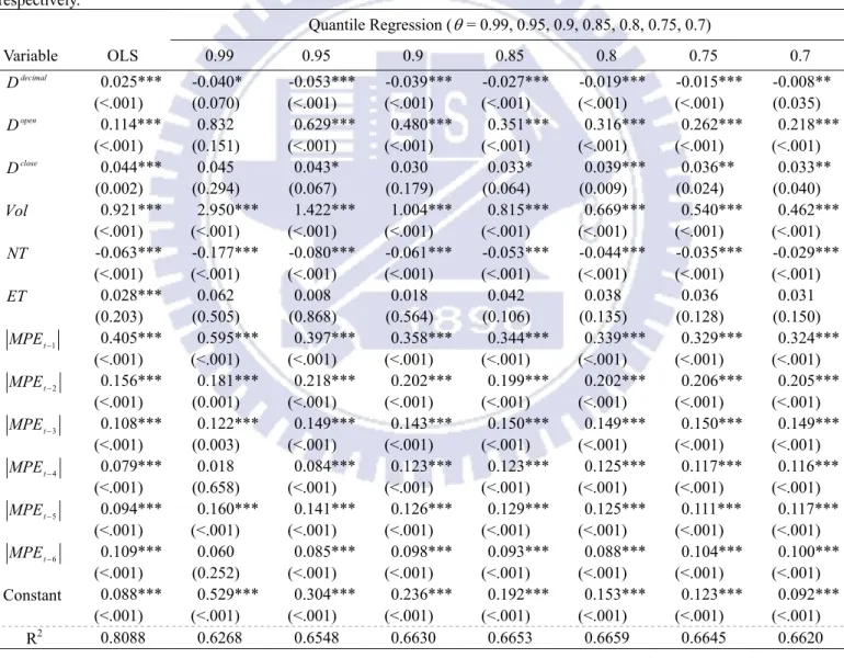
TABLE 6 MISPRICING ANALYSES FOR THE RELATIONSHIP BETWEEN SPDRS AND S&P 500 E-MINI FUTURES USING OLS AND QUANTILE REGRESSION... 30

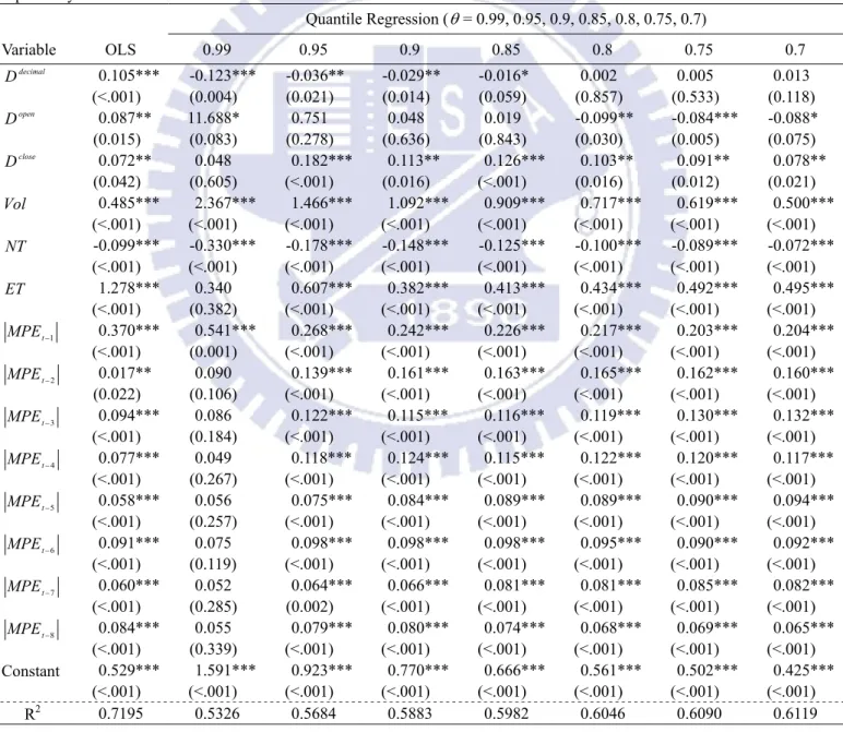
TABLE 7 MISPRICING ANALYSES FOR THE RELATIONSHIP BETWEEN QQQS AND NASDAQ 100 E-MINI FUTURES USING OLS AND QUANTILE REGRESSION... 33

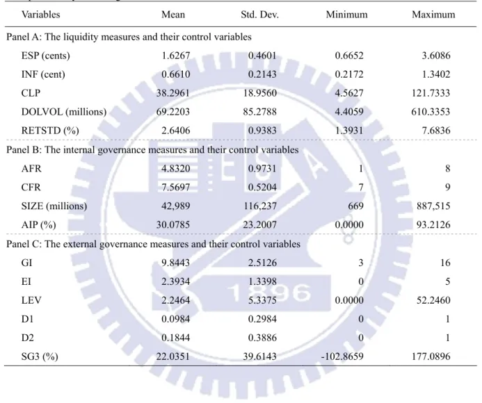
TABLE 8 DESCRIPTIVE STATISTICS OF ALL VARIABLES... 63

TABLE 9 PEARSON CORRELATION COEFFICIENTS OF ALL VARIABLES... 65

TABLE 10 OLS, 3SLS AND GMM ESTIMATION RESULTS OF THE EFFECTIVE SPREAD (ESP), ANNUAL BASIS S&P T&D FINAL RANKING (AFR) AND GOVERNANCE INDEX (GI) ... 69

TABLE 11 OLS, 3SLS AND GMM ESTIMATION RESULTS OF THE EFFECTIVE SPREAD (ESP), ANNUAL BASIS S&P T&D FINAL RANKING (AFR) AND ENTRENCHMENT INDEX (EI)... 70

TABLE 12 OLS, 3SLS AND GMM ESTIMATION RESULTS OF THE EFFECTIVE SPREAD (ESP), COMPOSITE BASIS S&P T&D FINAL RANKING (CFR) AND GOVERNANCE INDEX (GI) ... 71

TABLE 13 OLS, 3SLS AND GMM ESTIMATION RESULTS OF THE EFFECTIVE SPREAD (ESP), COMPOSITE BASIS S&P T&D FINAL RANKING (CFR) AND ENTRENCHMENT INDEX (EI) .... 72

TABLE 14 OLS, 3SLS AND GMM ESTIMATION RESULTS OF THE INFORMATION ASYMMETRY COMPONENT (INF), ANNUAL BASIS S&P T&D FINAL RANKING (AFR) AND GOVERNANCE INDEX (GI) ... 73

TABLE 15 OLS, 3SLS AND GMM ESTIMATION RESULTS OF THE INFORMATION ASYMMETRY COMPONENT (INF), ANNUAL BASIS S&P T&D FINAL RANKING (AFR) AND ENTRENCHMENT INDEX (EI)... 74

TABLE 16 OLS, 3SLS AND GMM ESTIMATION RESULTS OF THE INFORMATION ASYMMETRY COMPONENT (INF), COMPOSITE BASIS S&P T&D FINAL RANKING (CFR) AND GOVERNANCE INDEX (GI) ... 75

TABLE 17 OLS, 3SLS AND GMM ESTIMATION RESULTS OF THE INFORMATION ASYMMETRY COMPONENT (INF), COMPOSITE BASIS S&P T&D FINAL RANKING (CFR) AND ENTRENCHMENT INDEX (EI) ... 76

(9)

CHAPTER 1. INTRODUCTION

The phrase “market microstructure” is conceived by Garman (1976) as the title of his study about market marking and inventory costs. Later, the phrase evolved into a descriptive title for the investigation of the economic forces affecting trades, quotes and prices. Naturally, market microstructure can also be viewed as the branch of financial economics that investigates trading and organization of markets. About the previous studies on market microstructure issues, Biais et al. (2005) provide an excellent review of the literature by surveying topics about price formation and trading process, and the consequences of market organization for price discovery and welfare.

The organization of the market can be seen as the extensive form of the game played by investors and traders. It determines the way in which the private information and strategic behavior of the traders affect the market outcome. Like auction design or mechanism design, market microstructure analyzes how the rules of the game can be designed to minimize frictions and thus optimize the efficiency of the market outcome.

The rate of change in financial markets has accelerated in recent years, with an unprecedented proliferation of new markets and instruments. The goals of this research in microstructure are to improve the understanding of how markets work and to design well functioning markets. This dissertation focuses on several important issues in market microstructure, including tick size, arbitrage efficiency and market liquidity.

The first issue in this dissertation is to discuss the influences of tick size on arbitrage efficiency among markets. Tick size is the minimum price variation allowed for quoting and trading in financial assets, and refers to the smallest amount by which a trader may improve a price. For a considerable time, stocks on the New York Stock Exchange (NYSE) had been quoted in eighths of a dollar; however, on June 24, 1997, the NYSE reduced the tick size from

(10)

one eighth to one sixteenth. Starting from January 29, 2001, all stocks traded on the NYSE and on the American Stock Exchange (AMEX) have been subsequently quoted in decimals (i.e., penny pricing or decimalization). The decimalization of the stock markets represents an important issue for market participants because it had potentially significant influences on market efficiency and market liquidity, and therefore, the overall functioning of the financial markets.

After decimalization, arbitrageurs face higher execution risk because of the lower quoted depth and slower execution speed in the spot market. The financial issue that pricing efficiency and arbitrage opportunities between index futures and their underlying index surrounding decimalization will be important for market participants, since a structural change within one market may have significant impacts on the derivatives markets.

The second issue examined in this dissertation is the relationship between corporate governance and equity liquidity. Corporate governance is an extremely important issue for all investors. Within those firms where poor corporate governance is adopted, managers are more likely to use their information advantage to pursue a private benefit of control, which will ultimately lead to an increase in the agency costs faced by shareholders. As the agency problem worsens, insiders (such as executives or controlling owners) can easily exploit the wealth and the rights of small shareholders; it is for this reason that poor corporate governance is associated with all investors.

The information asymmetry component is a compensation arising from the asymmetric information risk faced by liquidity providers. Since it is difficult to determine who the informed traders are, the providers of liquidity cannot prevent the losses incurred when they actually trade with an informed trader. Effective spread must therefore include an appropriate information asymmetry component in order to compensate for this risk of loss, thereby enabling liquidity providers to maintain their operations against informed trading activities.

(11)

poor corporate governance and higher levels of asymmetric information risk; as a result, liquidity providers will tend to broaden the equity spread of those firms exhibiting poor corporate governance, since such price-protection action will have the effect of reducing the market liquidity of the stock. The effects of internal and external corporate governance mechanisms on equity liquidity, by using the S&P T&D rankings and governance index (entrenchment index) as proxies for internal and external corporate governance respectively, will reveal the importance of corporate governance to market participants.

All in all, the essays of this dissertation provide some insights into the issues of market microstructure, emphasize on the importance of tick size and corporate governance on financial markets. With these points in mind, the research results will furnish us with the empirical evidences to comprehend the occasion of some distinctive phenomena in financial markets.

(12)

(13)

CHAPTER 2. DECIMALIZATION AND THE ETFS AND

FUTURES PRICING EFFICIENCY

1. INTRODUCTION

Tick size is the minimum price variation allowed for quoting and trading in financial assets, and refers to the smallest amount by which a trader may improve a price.1 For some considerable time, stocks on the New York Stock Exchange (NYSE) had been quoted in eighths of a dollar; however, on June 24, 1997, the NYSE reduced the tick size from one eighth to one sixteenth. Starting from January 29, 2001, all stocks traded on the NYSE and on the American Stock Exchange (AMEX) were subsequently quoted in decimals (i.e., penny pricing or decimalization).2 The decimalization of the stock markets represents an important issue for market participants because it had potentially significant influences on market efficiency and market liquidity, and therefore, the overall functioning of the financial markets.

The decimalization of the US stock markets has attracted considerable research attention, albeit producing rather mixed results. Proponents of penny pricing argue that the reduction in tick size would improve market quality and liquidity. They suggest that a smaller tick size would benefit liquidity demanders as competition between liquidity providers increases, which would induce a reduction in overall bid-ask spreads (Bollen and Whaley, 1998; Ronen and Weaver, 2001; Henker and Martens, 2005). Bessembinder (2003) finds that not only small traders placing market orders have benefited, those traders executing large trades are also enjoying reductions in their average execution costs. Furfine (2003) also finds that after

1_{The tick size is normally set by exchange regulations.}

2_{The NYSE lowered the tick size to a penny for seven securities on August 28, 2000, for a further 57 securities} on September 25, 2000, and an additional 94 securities on December 5, 2000. All remaining securities began trading in decimals on January 29, 2001. NASDAQ began converting to decimal pricing on March 12, 2001, and completed the process on April 9, 2001.

(14)

decimalization, actively-traded stocks generally experience an increase in liquidity. Furthermore, Zhao and Chung (2006) find that decimal pricing led to a significant increase in the probability of information-based trading (PIN), arguing that decimal pricing increased the value of private information and raised the informational efficiency of asset price.

Opponents of penny pricing nevertheless argue that while such a change may have benefited certain liquidity demanders, this is to the detriment of liquidity providers. The increase in the costs of providing liquidity would lead to a decline in their willingness to provide liquidity (Harris, 1994; Glodstein and Kavajecz, 2000; Jones and Lipson, 2001; Bollen and Busse, 2006).

Graham et al. (2003) find that while the reduction in spreads reduces the trading costs for small trades, it has no effects on the trading costs for large trades, since the reduction in spreads is accompanied by a simultaneous reduction in depth. Chakravarty et al. (2004) argue that for institutional investors, the influence of penny pricing on trading costs is unclear, since their trades are typically large and require significant inroads into the limit order book, and/or the presence of other suppliers of liquidity, typically in the upstairs market. Furthermore, Bollen and Busse (2006) find that following the switch to decimals, actively-managed mutual funds experience an increase in trading costs.

Regarding the efficiency of the cash/futures pricing system, proponents of decimalization also argue that the lower transaction costs should result in a general reduction in index futures mispricing errors (which provide the trigger for arbitrage trading), because the finer increments of stock prices benefit investors as the pricing increment dictates the smallest possible bid-ask spread for a given stock. However, this particular viewpoint ignores the importance of possible reductions in liquidity due to penny pricing. Not only does decimalization lead to smaller spreads, but it can also cause a reduction in depth, which induces ambiguous changes in market quality.

(15)

Therefore, in order for an arbitrage trade to be profitable, the required positions taken by arbitrageurs are usually large, and thus, will normally require a deep market. Roll et al. (2005) argue that an illiquidity shock may have a lasting effect on arbitrage opportunities as arbitrageurs struggle to close the gap. They empirically demonstrate that market liquidity enhances the efficiency of the futures/cash pricing system.

In their study of the impact of decimalization on institutional traders, Chakravarty et al. (2005) find that decimalization appears to have benefited those institutions with greater patience, whereas it may have hurt those seeking quick execution of trades. Since arbitrageurs require quick execution of their submitted orders, and since they must also be well capitalized, this implies that arbitrageurs are more likely to be institutional investors that demand quick execution of their trades.3 Further, in order to cover transaction costs and make sufficient profits, arbitrageurs tend to take on large positions, which require a deep market. We therefore argue that after decimalization, the benefits obtained by the arbitrageurs, due to the reduction in the bid-ask spread, may have been more than offset by their losses stemming from the reduction in market depth, which may ultimately affect the ability and willingness of arbitrageurs to initiate arbitrage trades.

In this paper, we analyze market pricing efficiency in the pre- and post-decimalization periods by examining the arbitrage relationship between exchange-traded funds (ETFs) and index futures. There are three possible explanations from the literature as to why arbitrageurs’ profits may have suffered as a result of decimalization, as follows.

First of all, arbitrageurs require a deep market when engaging in arbitrage activities. They would be affected by the fall in liquidity if liquidity providers are less willing to provide it due to lowered profitability of supplying liquidity following the move to penny pricing (Anshuman and Kalay, 1998). Furthermore, arbitrageurs are essentially market makers who

3_{Attari et al. (2005) note that if arbitrageurs were not well capitalized, capital constraints would make their} trades predictable.

(16)

simultaneously connect buyers (sellers) in one market, with sellers (buyers) in another market, so they could also be viewed as porters of liquidity. Under normal circumstances, well-capitalized arbitrageurs act as suppliers of liquidity, with their presence being vital to the smooth functioning of the markets. Therefore, if market depth drops subsequent to penny pricing, it would impair the capabilities of arbitrageurs as suppliers or porters of liquidity in the markets.

Second, the execution risk would likely rise due to the reductions in average execution speed. A successful arbitrage trade carries almost no risk except for execution risks. Harris (1991) notes that a smaller tick size leads to an increase in the number of possible prices at which traders can trade, thereby complicating the negotiation process, and reducing the average speed of execution, which results in increased execution risk for arbitrageurs.

Third, a reduction in tick size may weaken the priority rules in the limit order book (Harris, 1994, 1996; Angel, 1997; Seppi, 1997). It lowers the cost of jumping ahead of existing orders in the book and gaining priority. It is likely that this activity, referred to as “front running”, would discourage investors from placing limit orders.4 Front-running tends to reduce the profits of informed traders.5 Harris (2003) argues that the long-run effect of front-running is to make prices less informative. Since front running limit orders placed by arbitrageurs became easier after decimalization, fewer arbitrageurs could consequently make profitable trades and they would have gradually withdrawn from the markets, which would ultimately make the market prices less informative. This implies that market efficiency would be impaired by decimalization.

After decimalization, arbitrageurs face higher execution risk because of decreased quoted depth and slower execution speed in the ETF market. We conjecture that the pricing efficiency

4_{Investors wary of front-runners would be more likely to conceal their true trading interest (depth) in a market} with a lower minimum price variation. Harris (1996) argues that the minimum price increment should be economically significant in order to protect liquidity providers from quote matchers.

5_{Harris (2003) defines informed traders as value traders, news traders, information-oriented technical traders} and arbitrageurs.

(17)

on average may have deteriorated in the post-decimalization period. Arbitragers will only participate in trading only when it is profitable to do so, meaning that only when the mispricing signal is large enough to compensate for the increased execution risk. Therefore, the pricing efficiency is likely to be improved when extreme mispricing signals occur. The purpose of this study is to examine pricing efficiency and arbitrage opportunities between index futures and their underlying index surrounding decimalization. Although many studies have been undertaken on the influence of tick reductions on the equity markets, only a few studies have examined pricing efficiency across related markets following tick reductions (see, for example, Henker and Martens, 2005; Chou and Chung, 2006). This is, however, an important topic, since a structural change within one market may have significant impacts on another.

As has been demonstrated in a number of the prior studies, penny pricing is likely to benefit certain traders while simultaneously hurting certain others. Our paper provides additional evidence on the merits of decimalization from the perspective of the efficacy of the cash/futures pricing system. We use ETFs as the index proxies, which include both the S&P 500 Depositary Receipts (SPDRs) and the NASDAQ 100 Index Tracking Stocks (QQQs).6 The sample index futures include the E-mini versions of the S&P 500 and NASDAQ 100 index futures.

Our study differs from the extant literature in the following ways. First of all, we analyze the influences of penny pricing on pricing efficiency across closely related markets; this is an area which has received relatively little attention in the literature. Examining the pre- and post-decimalization transmission of information between ETFs and index futures, Chou and Chung (2006) find that ETFs began to lead index futures in the price discovery process, and

6_{On November 9, 2004, NASDAQ and the AMEX announced that the NASDAQ 100 Index Tracking Stock} (listed under the symbol “QQQ”), would be transferred from the AMEX to NASDAQ effective from December 1, 2004, where it would trade under the new symbol “QQQQ”. In this study, we use the old symbol “QQQ”, because our sample period covers the time when the old symbol was in effect.

(18)

that there was also a tendency towards an increase in the information shares of ETFs after decimalization. However, they provide no evidence on the ways in which decimalization may have affected pricing efficiency from the perspective of arbitrage opportunities.

Secondly, our paper differs from Henker and Martens (2005), who study the spot-futures arbitrage during the pre- and post-introduction of sixteenths on the NYSE. Their focus is on the examination of the size of the theoretical mispricing signals (i.e., the ex-post arbitrage trading profits) with no consideration of either the transaction costs or the time lag involved in initiating arbitrage trades. Our study explicitly considers transaction costs while also measuring the profits from ex-ante arbitrage trading.

After observing a mispricing signal, arbitrageurs can only trade at the next available prices of ETFs and index futures; thus, when we refer to ex-ante arbitrage trading, we measure the arbitrage profits using the prices immediately after a mispricing signal is observed, as opposed to measuring the profit by the size of the mispricing signal. We believe that our analyses will more closely represent arbitrage profits in the real world and that they will provide valuable evidence on the changes in price efficiency as a result of penny pricing.

Finally, we analyze the regression of average pricing efficiency by the method of ordinary least squares (OLS), as well as the pricing efficiency of the entire distribution of mispricing sizes by the quantile regression. By controlling for the influence of the market characteristics on pricing efficiency, the OLS method would show the change in degree of mispricing on average; however, the quantile regression method could show the change in mispricing under various quantiles. Therefore, the quantile regression is particularly useful when we want to observe the change in pricing efficiency of the entire distribution of mispricing signals.

The remainder of this paper is organized as follows. Section 2 describes the data and discusses the research methodology. Section 3 presents the empirical results on the efficiency of the cash/futures pricing system between ETFs and E-mini futures by the ex-ante arbitrage

(19)

and the regression analyses. Finally, the conclusions are presented in Section 4.

2. DATA AND METHODOLOGY 2.1. The Data

Our analysis focuses on the arbitrage relationship between index ETFs and E-mini futures. ETFs are tradable instruments on the spot index, which makes arbitrage between the spot index and its underlying futures both simple and feasible. The sample ETFs include SPDRs and QQQs, and the sample E-mini futures include S&P 500 and NASDAQ 100 E-mini futures. The ETFs prices are usually scaled down in order to make them comparable to stock prices. The prices of SPDRs are 1/10th of the S&P 500 index level and the prices of QQQs are 1/40th of the NASDAQ 100 index level.7

The respective contract sizes of S&P 500 and NASDAQ 100 E-mini futures are $50 multiplied by the S&P 500 index level, and $20 multiplied by the NASDAQ 100 index level. Thus, for an arbitrage trade with a long or short position in one contract of S&P 500 E-mini futures (NASDAQ 100 E-mini futures), the required offsetting position in SPDRs (QQQs) is 500 (800) shares.

The sample covers the period July 27, 2000 to July 30, 2001, a period which spans six months prior to, and six months after, the date of decimalization.8 The data on ETFs, which include the tick-by-tick quote and trade prices, trading volume and quoted depth, are obtained from the NYSE Trade and Quote (TAQ) database. Only regular AMEX quote and trade prices are used for ETFs. The corresponding data on E-mini futures, which include trade prices and

7_{On February 14, 2000, NASDAQ announced that the Board of Directors of NASDAQ Investment Product} Services, Inc. (the sponsors of QQQs) had approved a two-for-one stock split. The payment date for the stock split was March 17, 2000, payable to all stockholders held on record as at February 28 2000. Therefore, the prices of QQQs became 1/40th_{of the index level form 1/20}th_{at this date of split.}

8_{On 31 July 2001, the NYSE began trading the DIAs, QQQs and SPDRs listed on the AMEX on the unlisted} trading privileges (UTP) basis. Boehmer and Boehmer (2003) showed that the introduction of UTP leads to an improvement in liquidity. In order to avoid any confounding effect, we confine our sample period up to this date.

(20)

number of trades, are obtained from the intraday database of Tick Data Inc..9 The ETF dividend data are obtained from the University of Chicago’s Center for Research in Security Prices database (CRSP). The three-month T-Bill rates on the secondary market, obtained from the web-based Federal Reserve Board database, are used as the risk-free rate (as a proxy for the opportunity costs of arbitrage trades).10 For the intraday analyses, we transform the daily T-Bill rates into continuous compounded rates, assuming constant rates within a day.

In order to ensure the accuracy of our sample data, we delete all trades and quotes that are out of time sequence. We also omit quotes that meet the following three conditions: (i) either the bid or the ask price is equal to, or less than, zero; (ii) either the bid or the ask depth is equal to, or less than, zero; and (iii) either the price or volume is equal to, or less than, zero.

Following Huang and Stoll (1996), we further minimize data errors by eliminating trades and quotes meeting the following additional criteria: (i) all quotes with negative bid-ask spreads, or with bid-ask spreads greater than US$4; (ii) all trades and quotes which took place either before the market opened or after it closed; (iii) all trade, bid and ask prices with consecutive absolute relative changes (i.e., absolute returns) of more than 10%.

The futures prices and ETF quotes are synchronized using the MINSPAN procedure suggested by Harris et al. (1995). We match every reported quote for an ETF with the trading price of an E-mini future so as to form trading pairs. If there is a futures trade at the exact time of the reported ETF quote, then a pair is formed; if there is no futures trade at the exact time of the reported ETF quote, the futures trades within the previous and subsequent seven seconds are then considered. When only one futures trade meets this criterion, a pair is formed. If both leading and lagging futures trades are obtained, the closer of the two trades is used to form the pair with the other trade being discarded.

Although, on each trading day, futures contracts continue to trade until 4:15 p.m. Eastern

9_{The quote data for index futures are unavailable, as is the case in most futures studies.}

(21)

Standard Time (EST), the trading pairs are only formed until 4:00 p.m. The number of matches equals the minimum total number of index futures trades and the minimum total number of ETF quotes. For SPDRs and S&P 500 E-mini futures, there are 301,018 observations in the pre-decimalization period and 322,524 in the post-decimalization period. For QQQs and NASDAQ 100 E-mini futures, there are 387,404 observations in the pre-decimalization period and 463,823 in the post-decimalization period.

2.2. Research Methodology

Using the cost-of-carry model, we establish the ex-post and ex-ante no arbitrage conditions between ETFs and E-mini futures. The focus of the ex-post tests is on the frequency and persistence of boundary violations, while the ex-ante tests calculate the arbitrage profits by explicitly considering the arbitrage trading lags and transaction costs. In a perfect market, the theoretical prices of index futures can be described by the cost-of-carry model, as follows:

( )

_t

[

_S

( )

_t _Div

( )

_t

]

_er(T t)

F = − − (1)

where F(t) is the theoretical futures price at time t for a contract expiring at time T; S(t) is the spot price of the underlying index at time t; r is the risk-free interest rate; and Div(t) is the present value of the dividend for holding the underlying index from time t to time T. In a perfect market, if prices deviate from Equation (1), then arbitrageurs will simultaneously sell the overpriced instrument and buy the underpriced one. This will ultimately bring the prices back to equilibrium.

The impact of transaction costs is to permit futures prices to fluctuate within a band around the theoretical price in Equation (1) without triggering profitable arbitrage opportunities, with the width of the band being dependent upon both the amount of the round-trip commission of trading spot and futures, and the size of the market impact of arbitrage trades. Most studies view such commission as a fixed cost; however, fees vary by

(22)

types of traders as well as by order size. The market impact costs can be measured by bid-ask spread and market depth. Taking transaction costs into consideration, Equation (2) describes the no-arbitrage band for the futures prices:

( )

[

]

( )

{

}

(

)

( )

{

[

( )

]

( )

}

₍

₎

m c t T r m c t T r _C _C _F _t _S _t _Div_t _e _C _C e t Div t S − − ₁− − < < − − ₁+ + ₍₂₎

where Cc and Cm represent commissions and market impact costs, respectively. If the futures

price penetrates the upper bound, a long arbitrage trade will simultaneously buy the spot and short the futures. If the futures price drops below the lower bound, a short arbitrage will make the reverse transactions.

2.2.1 Ex-Post Mispricing Analyses

We use ETFs as the cash proxy and E-mini futures as the sample futures contract. As argued by previous studies (Kurov and Lasser, 2002; Chu and Hsieh, 2002), the introduction of ETFs has provided index futures arbitrageurs with an easy way of taking advantage of arbitrage opportunities, and hence, has also improved price efficiency.

Assume that an arbitrage trade is placed at time t and lifted at the futures expiration date

T. With commissions and spread costs (proxy for the market impact costs), the no-arbitrage bands between SPDRs and S&P 500 E-mini futures (ES) are as shown in Equations (3) and (4):

( )

[

]

( )

{

}

(

c

)

( )

ask t T r bid SDiv t e C ES t t SPDR − − < × − ₁ 10 (3)

( )

[

]

( )

{

}

(

c

)

( )

bid t T r ask SDivt e C ES t t SPDR − + > × − ₁ 10 (4)

and the no-arbitrage band between QQQs and NASDAQ 100 E-mini futures (NQ) is as shown in Equations (5) and (6):

( )

[

]

( )

{

}

(

c

)

( )

ask t T r bid QDiv t e C NQ t t QQQ − − < × − ₁ 40 (5)

(23)

( )

[

]

( )

{

}

(

c

)

( )

bid t T r ask QDiv t e C NQ t t QQQ − + > × − ₁ 40 (6)

where SPDR(t)bid is the SPDR bid price, and SPDR(t)ask is the SPDR ask price, at time t. QQQ(t)bid is the QQQ bid price, and QQQ(t)ask is the QQQ ask price, at time t.

However, the bid and ask quotes for E-mini futures are unavailable. Kurov and Zabotina (2005) demonstrate the minimum E-mini futures bid-ask spread is binding. They estimate effective spreads for the E-mini futures using an average opposite direction absolute price change. We thus use the futures trade prices minus and plus one minimum tick size to proxy for the bid and ask prices of E-mini futures, respectively. Thus, ES(t)bid is the S&P 500 E-mini

bid price, and ES(t)ask is the S&P 500 E-mini ask price, at time t. NQ(t)bid is the NASDAQ

100 E-mini bid price and NQ(t)ask is the NASDAQ 100 E-mini ask price, at time t. SDiv(t)

and QDiv(t) are the respective present values of the dividends of SPDRs and QQQs, from time t to time T. As previously explained, since ETF prices are usually scaled down to make them comparable to those of stocks, adjusting factors of 10 and 40 are added.

We use the bid and ask prices to gauge the market impact costs, assuming that when trading in ETFs and E-mini futures, arbitrageurs can buy at the ask prices and sell at the bid prices. Thus, market impact costs are explicitly considered by the bid-ask spread. The transaction costs, Cc, in Equations (3), (4), (5) and (6) comprise of trading commissions only.

We adopt an approach similar to that of Chung (1991) and Chu and Hsieh (2002), in which several levels of commission are assumed when measuring the arbitrage profits. The levels of one-way transaction costs are set as from 0.05% to 0.5% of the theoretical futures price, with 0.05% increments.11

11_{Stoll and Whaley (1987) estimate that transaction costs are approximately 0.50-0.75% of the underlying index} value. Chung (1991) uses round-trip transaction costs ranging from 0.5 to 1.0% for MMI index arbitrages. Given a reasonable range of the index level, Klemkosky and Lee (1991) calculate that for S&P 500 index arbitrage, the transaction costs are about 0.14% for member firms and 0.24% for institutional investors. Sofianos (1993) assumes that round-trip transaction costs are roughly 0.4%. Neal (1996) estimates the average round-trip cost at 0.31% for buy programs and 0.32% for sell programs. Following Chu and Hsieh (2002) and Kurov and Lasser (2002), our specification of transaction costs covers most of these ranges.

(24)

2.2.2 Ex-Ant Arbitrage Profit Analyses

We further assume that arbitrageurs can trade at the next available ETF quote and futures trade prices immediately after observing a mispricing signal, which would yield more reasonable estimates of the profits that arbitrageurs are expected to make ex-ante. The respective ex-ante profits of long (ESAPL) and short (ESAPS) arbitrage trades, between

SPDRs and S&P 500 E-mini futures, are measured by Equations (7) and (8). Similarly, Equations (9) and (10) measure the ex-ante profits of long (NQAPL) and short (NQAPS)

arbitrage between QQQs and NASDAQ 100 E-mini futures.

( )

{

[

( )

]

( )

}

(

c

)

t T r ask bid L ES t SPDRt SDiv t e C ESAP = + − ₁₀× + − −+ ₁+ ₍₇₎

( )

[

]

( )

{

}

(

c

)

( )ask

t T r bid S SPDRt SDiv t e C ES t ESAP = 10× + − −+ 1− − + (8)

( )

{

[

( )

]

( )

}

(

c

)

t T r ask bid L NQt QQQt QDiv t e C NQAP = + − ₄₀× + − −+ ₁+ ₍₉₎

( )

[

]

( )

{

}

(

c

)

( )ask

t T r bid S QQQt QDivt e C NQt NQAP = 40× + − −+ 1− − + (10) where t+

indicates the time of the first quote (trade) price of ETFs (E-mini futures) immediately after the mispricing signal is observed, and all other variables are defined similarly as those in Equations (3) through (6).

2.2.3 Regression Analyses

Our empirical methodologies up to now focus on the ex-ante mispricing errors, which can be seen as univariate analyses. However, the changes in pricing efficiency can be affected by the changes in market factors other than decimalization. We thus follow Chung (1991) and Kurov and Lasser (2002) to control for other possible factors that are also likely to affect the market pricing efficiency. The simple version of the cost-of-carry model defined in Equation (1) is used to calculate the mispricing series. The mispricing series are calculated for every

(25)

5-minute interval.

We consider the change in average futures mispricing after the introduction of decimalization by using an autoregressive regression model, as defined in the following equation: t i i t i t t t close t open t decimal t t MPE ET NT Vol D D D MPE ε ϕ β β β β β β β τ + + + + + + + + =

∑

=1 − 6 5 4 3 2 1 0 (11)

where t denotes the 5-minute time interval. MPE_t is the average absolute pricing errors during time period t , defined similar to that in Kurov and Lasser (2002):

∑

= ∗ × − = n k tk k t k t t f ETF F F n MPE 1 , , , 1 (12)

where k denotes the kth price data within n observations in t time interval. F_t_,_k is the actual futures price, ∗

k t

F_, is the theoretical value from the cost-of-carry model, and f is the

adjusting factor for ETF_t_,_k prices. decimal t

D is a dummy variable that equals 0 for the pre-decimalization period and 1 afterward; open

t

D and close t

D are dummy variables indicating the opening and closing 5-minute intervals. Vol is the Parkinson (1980) extreme _t

value estimator to proxy for ETF volatility, defined as: 2 log 2 log 4 1 ⎟⎟ ⎠ ⎞ ⎜⎜ ⎝ ⎛ = t t t L H Vol (13)

where H and _t L denote the high and low prices of ETFs during time period t , _t

respectively. NT is the number of ETFs trades during time period t and _t ET is the _t

annualized time to expiration of the futures contract during time period t .

The dummy variable, decimal t

(26)

in mispricing after decimalization. A negative and significant coefficient of the dummy variable will indicate a decrease in average absolute mispricing and vise versa. The dummy variables open

t

D and close t

D are included in the regression to test whether mispricing is larger during the open and close intervals. The variables, Vol , _t ET , and _t NT , are used to control _t

for factors likely to affect pricing errors. The number of lagged error terms, τ , is equal to 6 and 8 periods for SPDRs and QQQs, respectively.12

Market volatility is an important factor affecting the mispricing of futures. Yadav and Pope (1994) show that futures’ mispricing tends to be higher during periods of high spot volatility. They argue that higher volatility makes arbitrage riskier by increasing uncertainty of arbitrage profits. Furthermore, Kurov and Lasser (2002) point out that when market risk is high enough, arbitrage trades will not be initiated even when they appear profitable, as arbitrageurs wait for even larger mispricing that serves as a “buffer” against risk. Chan and Chung (1993) demonstrate that increases in futures mispricing are followed by increases in volatility of spot and futures prices and the mispricing subsequently declines. Therefore, we expect a significant positive relation between volatility and pricing errors. Moreover, changes in spot trading volume may also affect the spot-futures pricing relation. Jones et al. (1994) show that number of trades contains most of the important information for describing trading activity. We conjecture that there is a significant negative relation between number of trades and average mispricing, as number of trades is a proxy for information arrivals.

In addition to the OLS method, to analyze the entire distribution of mispricing, we estimate Equation (11) by a linear quantile regression model proposed by Koenker and Bassett (1978). This approach permits estimating various quantile functions of a conditional distribution, among them, the median (0.5th quantile) function is a special case.13 Each

12_{We use the Durbin’s alternative statistic to test for the serial correlation problem. The test results indicate that} there are no first, second and third order serial correlation presented when the number of lag periods is set to 6 and 8 periods for SPDRs and QQQs, respectively.

(27)

quantile regression characterizes a particular (center or tail) point of a conditional distribution.14 The results from different quantile regressions provide a more complete description of the underlying conditional distribution of pricing errors.15

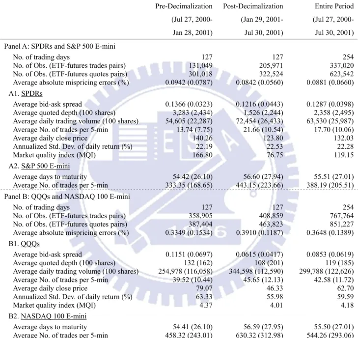
3. EMPIRICAL RESULTS 3.1. Summary Statistics

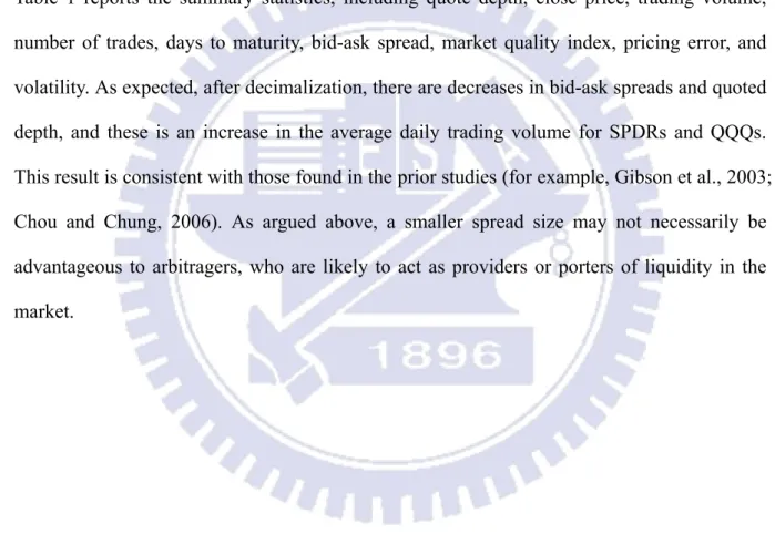
Table 1 reports the summary statistics, including quote depth, close price, trading volume, number of trades, days to maturity, bid-ask spread, market quality index, pricing error, and volatility. As expected, after decimalization, there are decreases in bid-ask spreads and quoted depth, and these is an increase in the average daily trading volume for SPDRs and QQQs. This result is consistent with those found in the prior studies (for example, Gibson et al., 2003; Chou and Chung, 2006). As argued above, a smaller spread size may not necessarily be advantageous to arbitragers, who are likely to act as providers or porters of liquidity in the market.

procedure is provided in Koenker (2005).

14_{We estimate two extreme quantiles, 0.01 and 0.99 quantiles, as well as 0.05 to 0.95 quantiles, with a 0.05} increment.

15_{Koenker and Hallock (2001) mention a faulty notion that quantile regression could be achieved by} segmenting the response variable into subsets according to its unconditional distribution and then doing least squares fitting on these subsets. They indicate that this form of “truncation on the dependent variable” would yield disastrous results. In general, such strategies are doomed to failure for all the reasons so carefully laid out in Heckman’s (1979) work on sample selection.

(28)

Table 1 Summary statistics

The table shows summary statistics for ETFs and their underlying E-mini futures. Quoted depth is calculated as (Qask + Qbid), and bid-ask spread is calculated as (Pask – Pbid), where Pask is the ask price, Pbid is the bid price, Qask is the depth at

ask and Qbid is the depth at bid. The market quality index (MQI) is calculated as [(Qask + Qbid)/10000/2]/[ (Pask – Pbid)/[( Pask + Pbid)/2] x 100] and the absolute mispricing error is calculated as |FM – FT|/(ETF x f ), where f is the

adjusting factor for ETF prices, FM is the futures market price, and FT is the futures theoretical price. Figures in

parentheses are standard deviation.

Pre-Decimalization (Jul 27, 2000-Jan 28, 2001) Post-Decimalization (Jan 29, 2001- Jul 30, 2001) Entire Period (Jul 27, 2000-Jul 30, 2001) Panel A: SPDRs and S&P 500 E-mini

No. of trading days 127 127 254 No. of Obs. (ETF-futures trades pairs) 131,049 205,971 337,020 No. of Obs. (ETF-futures quotes pairs) 301,018 322,524 623,542 Average absolute mispricing errors (%) 0.0942 (0.0787) 0.0842 (0.0560) 0.0881 (0.0660) A1. SPDRs

Average bid-ask spread 0.1366 (0.0323) 0.1216 (0.0443) 0.1287 (0.0398) Average quoted depth (100 shares) 3,283 (2,434) 1,526 (2,244) 2,358 (2,495) Average daily trading volume (100 shares) 54,605 (22,287) 72,454 (26,433) 63,530 (25,987) Average No. of trades per 5-min 13.74 (7.75) 21.66 (10.54) 17.70 (10.06) Average daily close price 140.26 123.80 132.03 Annualized Std. Dev. of daily return (%) 22.19 22.53 22.28 Market quality index (MQI) 166.80 76.75 119.15 A2. S&P 500 E-mini

Average days to maturity 54.42 (26.10) 56.60 (27.94) 55.51 (27.01) Average No. of trades per 5-min 333.35 (168.65) 443.15 (223.66) 388.19 (205.51) Panel B: QQQs and NASDAQ 100 E-mini

No. of trading days 127 127 254 No. of Obs. (ETF-futures trades pairs) 358,905 408,859 767,764 No. of Obs. (ETF-futures quotes pairs) 387,404 463,823 851,227 Average absolute mispricing errors (%) 0.3349 (0.1534) 0.3910 (0.1187) 0.3648 (0.1389) B1. QQQs

Average bid-ask spread 0.1151 (0.0697) 0.0615 (0.0417) 0.0853 (0.0619) Average quoted depth (100 shares) 132 (162) 108 (201) 119 (185) Average daily trading volume (100 shares) 254,978 (116,058) 344,598 (112,590) 299,788 (122,626) Average No. of trades per 5-min 39.52 (10.44) 45.65 (12.13) 42.58 (11.72) Average daily close price 79.07 46.33 62.70 Annualized Std. Dev. of daily return (%) 63.33 55.98 59.59 Market quality index (MQI) 4.37 4.01 4.18 B2. NASDAQ 100 E-mini

Average days to maturity 54.41 (26.10) 56.59 (27.95) 55.50 (27.01) Average No. of trades per 5-min 458.32 (243.01) 630.32 (312.98) 544.26 (293.06)

(29)

Previous studies on equity securities have demonstrated that there is a general reduction in the quoted depth after decimalization, and we also find this to be the case for both SPDRs and QQQs. Such reduction in market depth is likely to harm arbitrageurs, who usually trade large positions in order to realize the arbitrage profits. Even though the average quoted depth for both ETFs seem to be large, the standard deviation of quoted depth indicates that the quoted depth is quite volatile. Thus, it is very likely that arbitragers will experience times when the market depth is low and thus face high execution risk. This prompts us to empirically examine the arbitrage opportunity between ETFs and E-mini futures.

From Table 1, we find decrease (increase) in the average absolute mispricing errors for QQQs (SPDRs) after decimalization. From the summary statistics of pricing errors, it seems that no definite conclusions can be made regarding the cash/futures pricing efficiency after decimalization, which might be caused by failing to control for changes in other market factors, an issue will be addressed later by the method of OLS and quantile regressions. We further gauge the overall market quality by adopting a market quality index (MQI) similar to that proposed by Bollen and Whaley (1998). We define MQI in this study as the ratio between the half quoted depth of the prevailing bid-ask quotes and the percentage quoted spread. As can be seen from Table 1, there is a significant deterioration in market quality after decimalization, as measured by the MQI.

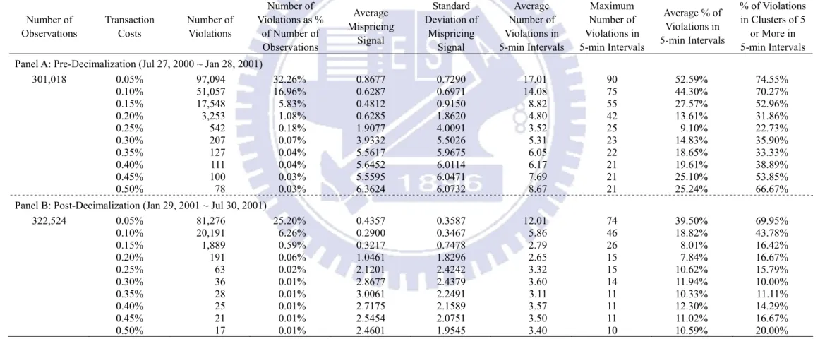
3.2. Ex-Post Mispricing Analyses

The mispricing signals are identified by Equations (3) and (4) for SPDRs and Equations (5) and (6) for QQQs with various levels of transaction costs based on the theoretical futures prices. The total number of violations, the number of violations as percentage of number of observations, the average mispricing signal, the standard deviation of signals, and the statistics of violation within a 5-minute interval, are summarized in Table 2 (for SPDRs), and Table 3 (for QQQs), for both the pre- and post-decimalization periods. As the tables show, an increase in

(30)

transaction costs tends to lead to reductions in the number of violations and the percentage of violations.

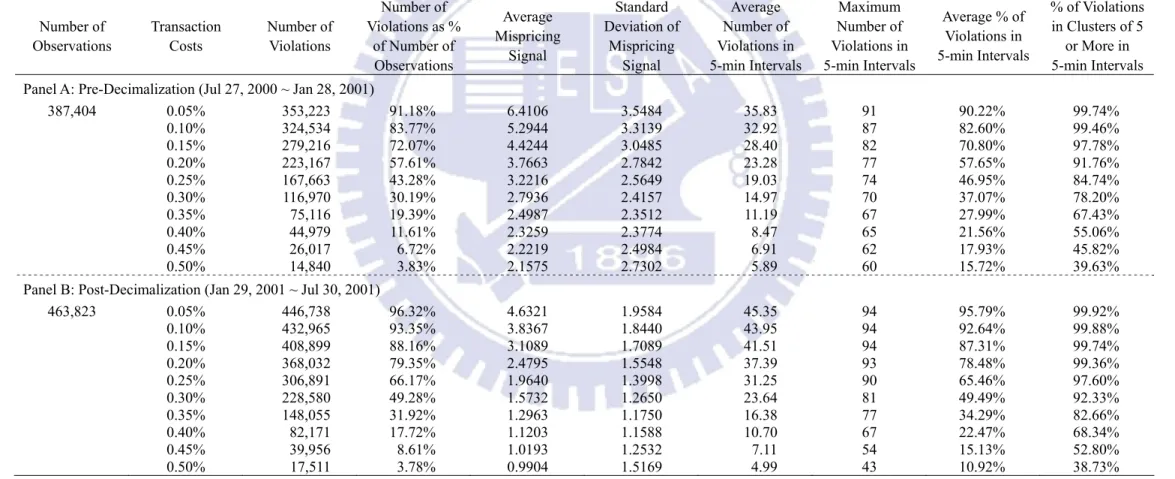
For SPDRs, comparing Panel A and Panel B of Table 2, we can see that after decimalization there is a substantial decrease in number of violations and the percentage of violations. In contrast, from Table 3, the number of violations and the percentage of violations generally increase for QQQs. As a result, no general conclusions regarding pricing efficiency can be made from the number and frequency of pricing errors.

The ex-post profit (i.e., the average mispricing signal) is defined as the difference between the futures quoted price and the appropriate upper or lower boundary when an mispricing signal is observed. When comparing the mispricing signal sizes in the pre- and post-decimalization periods, we find that the average signal sizes are generally smaller after penny pricing than before for both ETFs. It appears that the smaller mispricing signals indicate an improvement in pricing efficiency, but it is also likely that the somewhat smaller average signal sizes in the post-decimalization period are partially attributable to a reduction in the bid-ask spread. More importantly, a decreased mispricing size also implies that the potential arbitrage profits are smaller after decimalization, which may weaken arbitragers’ incentive to participate in trading.

Table 2 and Table 3 also show that most of the boundary violations before and after penny pricing are clustered. From Panel B in Table 2, for the case with transaction cost of 0.5%, although the total number of violations is only 17, the maximum number of violations in a 5-minute interval is as high as 10.16 Similar results are also obtained with various levels of transaction costs for both ETFs. This result supports the argument proposed by Chung (1991) that mispricing signals tend to occur in clusters.

16_{Note that the average number of violations in 5-minute intervals, the average percentage of violations in} 5-minute intervals and the percentage of violations in clusters of 5 or more in 5-minute intervals are calculated based on those 5-minute intervals with mispricing signals observed.

(31)

Table 2 Ex-post boundary violations of SPDRs and S&P 500 E-mini futures

The ex-post tests refer to the frequency and persistence of boundary violations. No-arbitrage boundaries are constructed with the SPDR and S&P 500 E-mini (ES) prices, which are defined as: ( ) ( )

[

]

( )

{

}

( c) ( )ask t T r bid SDivt e C ES t t SPDR − − < × − ₁ 10 or

{

[

( ) ( )

]

( )

}

( c) ( )bid t T r ask SDivt e C ES t t SPDR − + > × − ₁ 10

where SPDR(t)bid is the SPDR bid price and SPDR(t)ask is the SPDR ask price at time t; ES(t)bid is the S&P 500 E-minis bid price and ES(t)ask is the S&P 500 E-minis ask price at time t; SDiv(t)

refers to the present value of the SPDR dividend from time t to time T; and Cc is the trade commission. Since SPDR prices are 1/10th of the index level, an adjustment factor of 10 is applied.

Transaction costs are measured as a percentage of the theoretical futures value under the cost-of-carry model. Number of Observations Transaction Costs Number of Violations Number of Violations as % of Number of Observations Average Mispricing Signal Standard Deviation of Mispricing Signal Average Number of Violations in 5-min Intervals Maximum Number of Violations in 5-min Intervals Average % of Violations in 5-min Intervals % of Violations in Clusters of 5 or More in 5-min Intervals Panel A: Pre-Decimalization (Jul 27, 2000 ~ Jan 28, 2001)

301,018 0.05% 97,094 32.26% 0.8677 0.7290 17.01 90 52.59% 74.55% 0.10% 51,057 16.96% 0.6287 0.6971 14.08 75 44.30% 70.27% 0.15% 17,548 5.83% 0.4812 0.9150 8.82 55 27.57% 52.96% 0.20% 3,253 1.08% 0.6285 1.8620 4.80 42 13.61% 31.86% 0.25% 542 0.18% 1.9077 4.0091 3.52 25 9.10% 22.73% 0.30% 207 0.07% 3.9332 5.5026 5.31 23 14.83% 35.90% 0.35% 127 0.04% 5.5617 5.9675 6.05 22 18.65% 33.33% 0.40% 111 0.04% 5.6452 6.0114 6.17 21 19.61% 38.89% 0.45% 100 0.03% 5.5595 6.0471 7.69 21 25.10% 53.85% 0.50% 78 0.03% 6.3624 6.0732 8.67 21 25.24% 66.67%

Panel B: Post-Decimalization (Jan 29, 2001 ~ Jul 30, 2001)

322,524 0.05% 81,276 25.20% 0.4357 0.3587 12.01 74 39.50% 69.95% 0.10% 20,191 6.26% 0.2900 0.3467 5.86 46 18.82% 43.78% 0.15% 1,889 0.59% 0.3217 0.7478 2.79 26 8.01% 16.42% 0.20% 191 0.06% 1.0461 1.8296 2.65 15 7.84% 16.67% 0.25% 63 0.02% 2.1201 2.4242 3.32 15 10.62% 15.79% 0.30% 36 0.01% 2.8677 2.4379 3.60 14 11.94% 10.00% 0.35% 28 0.01% 3.0061 2.2491 3.11 11 10.33% 11.11% 0.40% 25 0.01% 2.7175 2.1589 3.57 11 12.30% 14.29% 0.45% 21 0.01% 2.5454 2.0751 3.50 11 11.02% 16.67% 0.50% 17 0.01% 2.4601 1.9545 3.40 10 10.59% 20.00%

(32)

Table 3 Ex-post boundary violations of QQQs and NASDAQ 100 E-mini futures

The ex-post tests refer to the frequency and persistence of boundary violations. No-arbitrage boundaries are constructed with the QQQ and NASDAQ E-mini (NQ) prices, which are defined as:

( )

[

]

( )

{

}

(

c

)

( )

ask t T r bid QDivt e C NQt t QQQ − − < × − ₁ 40 or

{

[

( )

]

( )

}

(

c

)

( )

bid t T r ask QDivt e C NQt t QQQ − + > × − ₁ 40

where QQQ(t)bid is the QQQ bid price and QQQ(t)ask is the QQQ ask price at time t; NQ(t)bid is the NASDAQ 100 E-minis bid price and NQ(t)ask is the NASDAQ 100 E-minis ask price at

time t; QDiv(t) refers to the present value of the QQQ dividend from time t to time T; and Cc is the trade commission. Since QQQ prices are 1/40th of the index level, an adjusting factor of

40 is applied. Transaction costs are measured as a percentage of the theoretical futures value under the cost-of-carry model. Number of Observations Transaction Costs Number of Violations Number of Violations as % of Number of Observations Average Mispricing Signal Standard Deviation of Mispricing Signal Average Number of Violations in 5-min Intervals Maximum Number of Violations in 5-min Intervals Average % of Violations in 5-min Intervals % of Violations in Clusters of 5 or More in 5-min Intervals Panel A: Pre-Decimalization (Jul 27, 2000 ~ Jan 28, 2001)

387,404 0.05% 353,223 91.18% 6.4106 3.5484 35.83 91 90.22% 99.74% 0.10% 324,534 83.77% 5.2944 3.3139 32.92 87 82.60% 99.46% 0.15% 279,216 72.07% 4.4244 3.0485 28.40 82 70.80% 97.78% 0.20% 223,167 57.61% 3.7663 2.7842 23.28 77 57.65% 91.76% 0.25% 167,663 43.28% 3.2216 2.5649 19.03 74 46.95% 84.74% 0.30% 116,970 30.19% 2.7936 2.4157 14.97 70 37.07% 78.20% 0.35% 75,116 19.39% 2.4987 2.3512 11.19 67 27.99% 67.43% 0.40% 44,979 11.61% 2.3259 2.3774 8.47 65 21.56% 55.06% 0.45% 26,017 6.72% 2.2219 2.4984 6.91 62 17.93% 45.82% 0.50% 14,840 3.83% 2.1575 2.7302 5.89 60 15.72% 39.63%

463,823 0.05% 446,738 96.32% 4.6321 1.9584 45.35 94 95.79% 99.92% 0.10% 432,965 93.35% 3.8367 1.8440 43.95 94 92.64% 99.88% 0.15% 408,899 88.16% 3.1089 1.7089 41.51 94 87.31% 99.74% 0.20% 368,032 79.35% 2.4795 1.5548 37.39 93 78.48% 99.36% 0.25% 306,891 66.17% 1.9640 1.3998 31.25 90 65.46% 97.60% 0.30% 228,580 49.28% 1.5732 1.2650 23.64 81 49.49% 92.33% 0.35% 148,055 31.92% 1.2963 1.1750 16.38 77 34.29% 82.66% 0.40% 82,171 17.72% 1.1203 1.1588 10.70 67 22.47% 68.34% 0.45% 39,956 8.61% 1.0193 1.2532 7.11 54 15.13% 52.80% 0.50% 17,511 3.78% 0.9904 1.5169 4.99 43 10.92% 38.73%

(33)

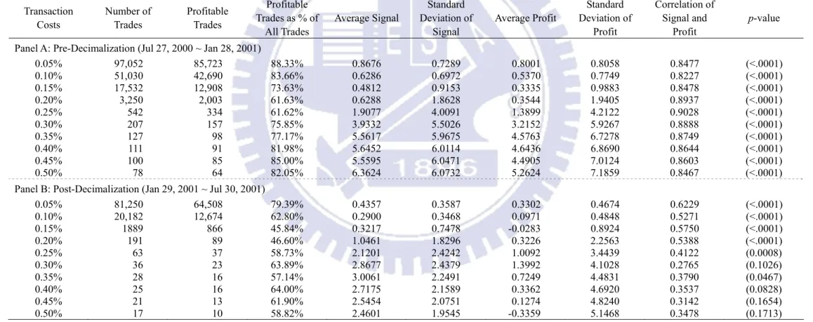
Table 4 Ex-ante arbitrage analyses for SPDRs and S&P 500 E-mini futures

The ex-ante tests impose an execution lag for trading in SPDRs and S&P 500 E-mini futures, and thus the ex-ante mean profits are arbitrage profits after considering the transaction lag. A long arbitrage (ESAPL), triggered by futures overpricing, buys 500 SPDR shares and shorts an S&P 500 E-mini futures contract after observing an upper-boundary violation, whereas a short

arbitrage (ESAPS), triggered by futures underpricing, executes the reverse transactions. Profits for long and short arbitrage are measured as:

( )

{

[

( )

]

( )

}

₍

₎

c t T r ask bid L ESt SPDRt SDivt e C ESAP = ₊ − × ₊ − ₊ ₋+ + 1 10 and

{

[

( )

]

( )

}

(

c

)

( )

ask t T r bid S SPDRt SDivt e C ESt ESAP ₌ _× + ₋ + −+ ₋ ₋ + 1 10

where t+ indicates the time of the first quote (trade) price of ETFs (E-minis) immediately after observation of the mispricing signal. SPDR(t+)bid is the SPDR bid price and SPDR(t+)ask is the

SPDR ask price at time t+. ES(t+)bid is the S&P 500 E-mini futures bid price and ES(t+)ask is the S&P 500 E-mini futures ask price at time t+; SDiv(t+) refers to the present value of the SPDR

dividend from time t+ to time T; and Cc is the trade commission. Since SPDR prices are 1/10th of the index level, an adjustment factor of 10 is applied.

Transaction Costs Number of Trades Profitable Trades Profitable Trades as % of All Trades Average Signal Standard Deviation of Signal Average Profit Standard Deviation of Profit Correlation of Signal and Profit p-value

Panel A: Pre-Decimalization (Jul 27, 2000 ~ Jan 28, 2001)

0.05% 97,052 85,723 88.33% 0.8676 0.7289 0.8001 0.8058 0.8477 (<.0001) 0.10% 51,030 42,690 83.66% 0.6286 0.6972 0.5370 0.7749 0.8227 (<.0001) 0.15% 17,532 12,908 73.63% 0.4812 0.9153 0.3335 0.9883 0.8478 (<.0001) 0.20% 3,250 2,003 61.63% 0.6288 1.8628 0.3544 1.9405 0.8937 (<.0001) 0.25% 542 334 61.62% 1.9077 4.0091 1.3899 4.2122 0.9028 (<.0001) 0.30% 207 157 75.85% 3.9332 5.5026 3.2152 5.9267 0.8888 (<.0001) 0.35% 127 98 77.17% 5.5617 5.9675 4.5763 6.7278 0.8749 (<.0001) 0.40% 111 91 81.98% 5.6452 6.0114 4.6436 6.8690 0.8644 (<.0001) 0.45% 100 85 85.00% 5.5595 6.0471 4.4905 7.0124 0.8603 (<.0001) 0.50% 78 64 82.05% 6.3624 6.0732 5.2624 7.1859 0.8467 (<.0001)

0.05% 81,250 64,508 79.39% 0.4357 0.3587 0.3302 0.4674 0.6229 (<.0001) 0.10% 20,182 12,674 62.80% 0.2900 0.3468 0.0971 0.4848 0.5271 (<.0001) 0.15% 1889 866 45.84% 0.3217 0.7478 -0.0283 0.8924 0.5750 (<.0001) 0.20% 191 89 46.60% 1.0461 1.8296 0.3226 2.2563 0.5388 (<.0001) 0.25% 63 37 58.73% 2.1201 2.4242 1.0092 3.4439 0.4122 (0.0008) 0.30% 36 23 63.89% 2.8677 2.4379 1.3992 4.1028 0.2765 (0.1026) 0.35% 28 16 57.14% 3.0061 2.2491 0.7249 4.4831 0.3790 (0.0467) 0.40% 25 16 64.00% 2.7175 2.1589 0.3362 4.6920 0.3537 (0.0828) 0.45% 21 13 61.90% 2.5454 2.0751 0.1274 4.8240 0.3142 (0.1654) 0.50% 17 10 58.82% 2.4601 1.9545 -0.3359 5.1468 0.3478 (0.1713)

(34)

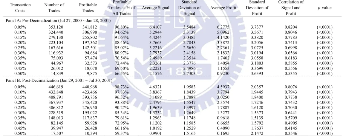
Table 5 Ex-ante arbitrage analyses for QQQs and NASDAQ 100 E-mini futures

The ex-ante tests impose an execution lag for trading QQQs and NASDAQ 100 E-mini futures, and thus the ex-ante mean profits are arbitrage profits after considering the transaction lag. A long arbitrage (NQAPL), triggered by futures overpricing, buys 800 QQQ shares and shorts a NASDAQ 100 E-mini futures contract after the observation of an upper-boundary violation,

whereas a short arbitrage (NQAPS), triggered by futures underpricing, executes the reverse transactions. Profits for the long and short arbitrage are measured as:

( )

{

[

( )

]

( )

}

₍

₎

c t T r ask bid L NQt QQQt QDivt e C NQAP = ₊ − × ₊ − ₊ ₋+ + 1 40 and

{

[

( )

]

( )

}

(

c

)

( )

ask t T r bid S QQQt QDivt e C NQt NQAP ₌ _× + ₋ + −+ ₋ ₋ + 1 40

where t+ indicates the time of the first quote (trade) price of ETFs (E-minis) immediately after observation of the mispricing signal. QQQ(t+)bid is the QQQ bid price and QQQ(t+)ask is the

QQQ ask price at time t+. NQ(t+)bid is the NASDAQ 100 E-mini futures bid price and NQ(t+)ask is the NASDAQ 100 E-mini futures ask price at time t+; QDiv(t+) refers to the present value

of the QQQ dividend from time t+ to time T; and Cc is the trade commission. Since QQQ prices are 1/40th of the index level, an adjustment factor of 40 is applied.

Transaction Costs Number of Trades Profitable Trades Profitable Trades as % of All Trades Average Signal Standard Deviation of Signal Average Profit Standard Deviation of Profit Correlation of Signal and Profit p-value

Panel A: Pre-Decimalization (Jul 27, 2000 ~ Jan 28, 2001)

0.05% 353,120 341,812 96.80% 6.4107 3.5484 6.2775 3.7377 0.8204 (<.0001) 0.10% 324,440 306,998 94.62% 5.2944 3.3139 5.0962 3.5671 0.8046 (<.0001) 0.15% 279,138 255,802 91.64% 4.4244 3.0485 4.1420 3.3820 0.7783 (<.0001) 0.20% 223,104 197,362 88.46% 3.7663 2.7843 3.3872 3.2056 0.7413 (<.0001) 0.25% 167,616 142,501 85.02% 3.2216 2.5650 2.7361 3.0725 0.6998 (<.0001) 0.30% 116,932 94,684 80.97% 2.7937 2.4158 2.1832 3.0194 0.6566 (<.0001) 0.35% 75,093 57,474 76.54% 2.4989 2.3514 1.7402 3.0558 0.6183 (<.0001) 0.40% 44,967 32,573 72.44% 2.3261 2.3776 1.4054 3.1803 0.5855 (<.0001) 0.45% 26,012 18,078 69.50% 2.2221 2.4986 1.1553 3.3699 0.5556 (<.0001) 0.50% 14,839 9,875 66.55% 2.1576 2.7303 0.9230 3.6393 0.5355 (<.0001)

0.05% 446,619 440,968 98.73% 4.6321 1.9583 4.5937 2.0357 0.8076 (<.0001) 0.10% 432,848 423,466 97.83% 3.8367 1.8439 3.7794 1.9445 0.7943 (<.0001) 0.15% 408,791 393,736 96.32% 3.1089 1.7088 3.0250 1.8400 0.7738 (<.0001) 0.20% 367,937 345,420 93.88% 2.4794 1.5547 2.3574 1.7246 0.7432 (<.0001) 0.25% 306,812 276,950 90.27% 1.9639 1.3997 1.7887 1.6120 0.7030 (<.0001) 0.30% 228,519 195,022 85.34% 1.5732 1.2649 1.3277 1.5373 0.6441 (<.0001) 0.35% 148,013 117,837 79.61% 1.2963 1.1748 0.9618 1.5139 0.5709 (<.0001) 0.40% 82,145 59,928 72.95% 1.1202 1.1585 0.6655 1.5792 0.4905 (<.0001) 0.45% 39,947 26,428 66.16% 1.0192 1.2529 0.4090 1.7637 0.4145 (<.0001) 0.50% 17,507 10,394 59.37% 0.9901 1.5165 0.1695 2.1472 0.3546 (<.0001)

(35)

3.3. Ex-Ante Arbitrage Profit Analyses

In this section, we report the results of the ex-ante analyses under the assumption that arbitragers can only transact at the next available futures trade price and ETF quote price after observing a mispricing signal.17 Table 4 and Table 5 present the results for SPDRs and QQQs surrounding decimalization, respectively. As Table 4 shows, under different levels of transaction costs, there are significant decreases in the number and percentage of profitable trades for SPDRs after decimalization. Table 5, on the contrary, shows substantial increases in the number and percentage of profitable trades for QQQs after decimalization.

It would seem, therefore, that there are no consistent results in the frequencies of profitable trades after the reduction in tick size. Nevertheless, from Table 4 and Table 5, it is seen that the ex-ante mean arbitrage profits decrease for both SPDRs and QQQs, and the correlation of signal and profit is lower after penny pricing. Interestingly, the decreases in mean arbitrage profits are relatively more significant at higher levels of transaction costs, when the required mispricing signals are large. This indicates that pricing efficiency changes are likely to be different for mispricing signals of different sizes.

These seem to indicate that the efficiency of market pricing may have been improved as a result of decimalization. However, the decrease in minimum tick size makes the boundary conditions to be tighter and tends to make smaller mispricing signals, thus a decrease in mispricing signals also implies that the mean arbitrage profits after decimalization are lower and this does not necessarily indicate an improvement in pricing efficiency. We suggest that the decreases in mispricing signals and mean arbitrage profits are caused, at least partially, by the narrower spreads of ETFs in the post-decimalization period. However, due to the simultaneous reduction in quoted depth, and the increase in execution risk, it is much more

17_{The assumption of trading at the next available quotes should be reasonable because the average time span} between the tick-by-tick trades are about 9.46 and 6.94 seconds for SPDRs and QQQs, respectively, which would be sufficient for arbitragers that closely monitor the market conditions to react to the mispricing signals.

金融市場微結構之探討：升降單位與流動性議題之分析

國

立

交

通

大

學

管理科學系

博

士

論

文

No. 28

金融市場微結構之探討：升降單位與流動性議題之分析

Essays on the Microstructure Issues of Tick Size and Equity Liquidity

研 究 生：陳煒朋

指導教授：鍾惠民 教授

Essays on the Microstructure Issues of Tick Size and Equity Liquidity

研 究 生：陳煒朋 Student: Wei-Peng Chen

指導教授：鍾惠民 博士 Advisor: Dr. Huimin Chung

國 立 交 通 大 學

管 理 科 學 系

財 務 金 融 組

博 士 論 文

金融市場微結構之探討：升降單位與流動性議題之分析

研究生：陳煒朋 指導教授：鍾惠民 博士

國立交通大學管理科學系財務金融組博士班

中文摘要

Essays on the Microstructure Issues of Tick Size and

Equity Liquidity

Student: Wei-Peng Chen Advisor: Dr. Huimin Chung

Finance Division

Department of Management Science

National Chiao Tung University

ABSTRACT

ACKNOWLEDGEMENTS

TABLE OF CONTENTS

LIST OF TABLES

CHAPTER 1. INTRODUCTION

CHAPTER 2. DECIMALIZATION AND THE ETFS AND

FUTURES PRICING EFFICIENCY

( )

[

( )

( )

]

( )

( )

[

]

{

}

(

)

( )

{

[

( )

( )

]

}

(

)

( )

( )

[

]

{

}

(

)

( )

( )

( )

[

]

{

}

(

)

研究生：陳煒朋

指導教授：鍾惠民教授

研究生：陳煒朋 Student: Wei-Peng Chen

指導教授：鍾惠民博士 Advisor: Dr. Huimin Chung

國立交通大學

管理科學系

財務金融組

博士論文

研究生：陳煒朋指導教授：鍾惠民博士

₍

₎