國
立
交
通
大
學
資訊科學與工程研究所
碩
士
論
文
針對多重通道的無線網狀網路,整合動態頻
段分配和路由選擇協定以解決節點失聰問
題
Combining dynamic channel assignment and routing
protocol for solving deafness problems in multi-channel
wireless mesh networks
研 究 生:張瑋倫
指導教授:簡榮宏 教授
針對多重通道的無線網狀網路,整合動態頻段分配和路由選擇協定以
解決節點失聰問題
Combining dynamic channel assignment and routing protocol for solving
deafness problems in multi-channel wireless mesh networks
研 究 生:張瑋倫 Student:Wei-Lun Chang
指導教授:簡榮宏 Advisor:Rong-Hong Jan
國 立 交 通 大 學
資 訊 科 學 與 工 程 研 究 所
碩 士 論 文
A ThesisSubmitted to Institute of Computer Science and Engineering College of Computer Science
National Chiao Tung University in partial Fulfillment of the Requirements
for the Degree of Master
in
Computer Science
July 2006
針對多重通道的無線網狀網路,整合動態頻段分配和
路由選擇協定以解決節點失聰問題
研究生:張瑋倫
指導教授:簡榮宏 博士
國立交通大學資訊科學與工程研究所
摘
要
近年來因為無線網路的便利性和可攜帶性,使用無線網路作為溝通的媒介, 已經越來越普及。因此,當多人同時使用無線網路時,提高傳送的頻寬是非常重 要議題。在 IEEE 802.11 無線網路上,雖然擁有多個不會互相干擾的頻段。但在 此協定中,所有的使用者卻只能利用相同頻段來存取無線網路。如此會造成相同 頻段上嚴重的干擾,使得傳送頻寬下降。在多重頻段、單一天線的網狀網路環境 下,可以使用動態的頻段分配來減低干擾,增加傳輸頻寬。但動態的頻段分配將 會產生節點失聰的問題,這是因為傳送方和接收方彼此都可能會改變頻段。So 和 Vaidya 提出一結合動態頻段分配和路由選擇的協定,來解決此節點失聰問題。 但此方法侷限在同一路由路徑須使用相同頻段,因而降低了頻段使用效能。本篇 論文針對此一問題,提出一個新的結合動態頻段分配和路由選擇方法,讓同一路 由路徑可以使用一個以上的頻段來增進系統效能。除此之外,我們亦改進 So 和 Vaidya 的方法,讓傳輸頻寬做進一步的提升Combining dynamic channel assignment and routing
protocol for solving deafness problems in multi-channel
wireless mesh networks
Student:Wei-Lun Chang
Advisor:Dr. Rong-Hong Jan
I
NSTITUTE OF
C
OMPUTER
S
CIENCE AND
E
NGINEERING
N
ATIONAL
C
HIAO
T
UNG
U
NIVERSITY
Abstract
Abstract— In the recent years, because of convenience and portability in the wireless network, wireless communications become more and more popular. It is important to increase the network throughput when the number of users becomes higher. In the IEEE 802.11 standard, it provides multiple orthogonal channels, but all users can only access the same channel for data transmissions. This situation causes the high co-channel interference to decrease the network throughput. In a multi-channel single-radio environment, dynamic channel assignment can help to decrease interference and increase network throughput. However, dynamic channel assignment will suffer the deafness problem. It is because both sender and receiver may change their channels without informing each other. So and Vaidya proposed a protocol which combines dynamic channel assignment and routing protocol to solve the deafness problem. However, this method restricts on assigning the same channel on the routing path which decreases the channel utilization. In this thesis, we propose a new method which combines dynamic channel assignment and routing protocol to assign more than one channel on the routing path to improve network performance. Besides, we also enhance So and Vaidya’s method to increase the transmission bandwidth.
Contents
1 Introduction 6 2 Related Works 9
2.1 Single-Channel Single-Radio Environment . . . 9
2.2 Multi-Channel Single-Radio Environment . . . 10
2.3 A Previous Work to Solve The Deafness Problem . . . 13
2.4 Disadvantages of MCRP . . . 17
3 Modified-MCRP 20 3.1 MCRP . . . 20
3.1.1 Node Classification . . . 20
3.1.2 Gather Channel Usage Information in Each Node’s Neigh-borhood . . . 21
3.1.3 Route Discovery . . . 22
3.2 Enhanced MCRP (EMCRP) . . . 27
3.2.1 Node Classification . . . 28
3.2.2 Route Discovery . . . 29
3.3 Split Enhanced MCRP (SEMCRP) . . . 31
4 Simulation 51 5 Conclusion and Future Work 57
List of Figures
1.1 The illustration of routing metrics on links. . . 7
2.1 The illustration of co-channel interference. . . 10
2.2 The illustration of the deafness problem. . . 12
2.3 The initial random channel assignment in MCRP. . . 15
2.4 The way to send RREQ in MCRP. . . 15
2.5 The way to send RREP in MCRP. . . 16
2.6 Node C has the deafness problem. . . 16
2.7 Switching node C changes its channel from 1 to 2. . . 18
2.8 Switching node C changes its channel from 2 to 1. . . 19
2.9 Two adjacent switching nodes will cause the deafness problem. . . 19
3.1 Four kinds of node states . . . 21
3.2 Flow table in each node . . . 22
3.3 Each node sets up its own flow table . . . 23
3.4 Channel table in RREQ . . . 23
3.5 The procedure of updating channel table and flow table from A to D 25 3.6 Traffic flow from A to D can assign channel 2 or channel 3 . . . 26
3.7 Destination node G can choose one of the routing paths with the lowest interference one . . . 27
3.8 MCRP discards the feasible channel 3 . . . 28
3.9 Sender’s channel and state information . . . 30
3.10 Rules to generate and update channel table in RREQ . . . 39
3.11 EMCRP updates channel table from source to destination . . . 40
3.12 The dotted traffic flow can be assigned channel 3 without the deaf-ness problem . . . 40
3.13 MCRP or EMCRP can assign all channels with the same bottleneck channel load 1 . . . 41
3.14 SEMCRP can assign channel 3 from F to H, and channel 1 from H to J with the bottleneck channel load 0 . . . 42
3.15 MCRP can’t find any feasible channels on the dotted routing path . 42 3.16 Split Enhanced MCRP can find a feasible channel assignment on the routing path . . . 43
3.17 Destination F will have channel, flow and state information of all nodes on the routing path . . . 44
3.18 Destination node F sets up the front table . . . 45
3.19 Destination node F sets up the rear table . . . 45
3.20 Rules to generate and update the front table . . . 46
3.21 Rules to generate and update the rear table . . . 47
3.22 Front split table and rear split table . . . 48
3.23 Destination node F sets up the front split table . . . 48
3.24 Destination node F sets up the rear split table . . . 48
3.25 The routing path is from A to F,A to C is on channel 1; C to F is on channel 3 . . . 48
3.26 The routing path is from A to F, A to D is on channel 2; D to F is
on channel 3 . . . 49
3.27 Both two channel assignments have the same bottleneck load 3 . . . 50
4.1 100 nodes grid topology . . . 53
4.2 49 nodes grid topology . . . 54
4.3 Network throughput with different number of flows . . . 55
4.4 Network throughput with different traffic rates . . . 55
Chapter 1
Introduction
Recently, wireless network is more and more popular. Because it supports high mobility, using wireless network is more convenient than using wired network. The maximum transmission rate of wireless local area network (WLAN) has been improved from 11Mbps (802.11b) to 54Mbps (802.11a). The high transmission rate means short transmission delay. In the IEEE 802.11 network, because all nodes use the same channel to access the network, the co-channel interference is direct proportion to the number of users in the network. As a result, many routing and channel assignment protocols have been proposed to reduce the co-channel interference.
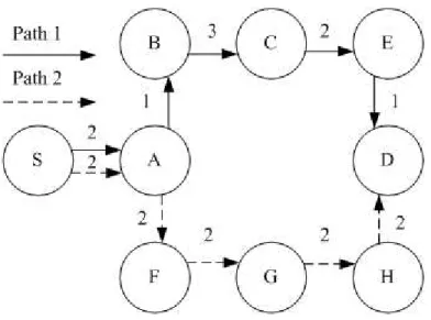
In single channel environment, routing protocols with new metrics can help to reduce the co-channel interference. Some pervious works [1, 2, 3, 4, 5, 6] pro-posed routing metrics with considering interference to find better routing paths. For example, in Figure 1.1, there are two routing paths which can be chosen from source to destination. We can choose a least interference path, according to the metrics on links.
Figure 1.1: The illustration of routing metrics on links.
Other routing protocols with link schedule to decrease the interference. The main idea is to activate links at different time slots which can decrease the co-channel interference. Although link schedule can help to decrease the interference, each node needs to maintain time synchronization. For wireless network, it is known that maintaining the time synchronization is difficult.
In multiple channels environment, such as multi-channel wireless mesh net-works, we can assign orthogonal channels to different nodes to decrease the co-channel interference. Only nodes with the same co-channels will interfere with each other when they are in the interference range.
In multi-channel wireless networks, because the channel switching delay is very short (e.g. 80µs) [7], this thesis presents a dynamic channel assignment to improve the network performance. For easy to implement in the future, we do not consider the link schedule method in our protocol which needs to maintain time
synchronization for all nodes. However, the dynamic channel assignment without link schedule will cause the deafness problem. The deafness problem happens when sender and receiver are both on different channels causing transmission failures to decrease the network throughput. In this thesis, we also propose a method to solve the deafness problem. In the next chapter, the deafness problem will be discussed in detail.
The outline of the rest in this thesis is as follows. In Chapter 2, we discuss several routing and channel assignment protocols in multi-channel single-radio en-vironment. In Chapter 3, we present our methods for channel assignment. In Chapter 4, we show our performance is better than pervious works in simulation. In Chapter 5, the conclusion and the direction of future works are given.
Chapter 2
Related Works
In this chapter, we discuss pervious works about increasing the wireless net-work throughput by designing channel assignment or routing protocols. In wireless local area network, we classify the network environment into two parts. Single-Channel Single-Radio (SCSR) and Multi-Single-Channel Single-Radio (MCSR) are two network environments of pervious works for increasing throughput. We will show their methods in different network models as follows.
2.1
Single-Channel Single-Radio Environment
In SCSR environment, channel assignment protocols can’t improve the net-work throughput at all. As a result, we only consider routing protocols here. In traditional routing protocols, hop count is the most common metric. However, us-ing hop count would cause the hot spot problem, and it doesn’t consider packet loss ratio on links. This routing metric won’t have a good performance in throughput. Therefore, many new routing metrics considering link transmission rate [1, 2], packet loss ratio [3, 4, 5], or co-channel interference [6] are proposed. Low packet loss ratio, low co-channel interference and high transmission rate on links all help
to increase the throughput. As a result, those new metrics all cause a better per-formance than the traditional hop count metric.
Besides, there are some routing protocols using the link schedule method [8, 9] to improve throughput. The main idea is to let links interfering with each other won’t be active at the same time. Although routing protocols with the link schedule method can increase throughput, it needs to maintain all nodes’ time synchronization which is hard to implement in wireless networks.
2.2
Multi-Channel Single-Radio Environment
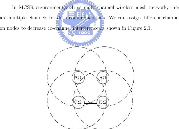
In MCSR environment,such as multi-channel wireless mesh network, there are multiple channels for data communications. We can assign different channels on nodes to decrease co-channel interference as shown in Figure 2.1.
In Figure 2.1, there are four nodes A, B, C and D. In each node’s interfer-ence range, they can’t transmit on the same channel at the same time. Therefore, link AB and CD can’t transmit simultaneously in traditional SCSR environment. However, in multi-channel environment, we can assign A, B on channel 1 and C, D on channel 2. This simple channel assignment can let link AB and CD transmit at the same time without collisions.
Many channel assignment protocols have been proposed to improve net-work throughput in MCSR environment. We classify them into two parts, static channel assignment and dynamic channel assignment. Static channel assignment means nodes need to stay on a fixed channel, and dynamic channel assignment allows nodes can switch to different channels.
In single-radio environment, static channel assignment may not have a good performance in throughput. Although assigning different channels can decrease co-channel interference as shown in figure 2.1, it would cause connectivity problem from A to D. Because A and C on different channels can’t communicate with each other, B and D on different channels also can’t communicate either. Because there is no routing path from A to D, static channel assignment is not suitable in MCSR environment to increase throughput.
In dynamic channel assignments, we can also classify these assignments into two parts, negotiation-based and receiver-based channel assignment. Both of them can utilize multiple channels to increase the network throughput without the con-nectivity problem.
In negotiation-based channel assignments, such as [10, 11], sender and re-ceiver both tune to the same control channel at the same time to negotiate a data channel before each transmission. Because each communication chooses a data channel dynamically, it is suitable in unstable network environment, such as nodes with high mobility. On the other hand, because all nodes tune to the same com-mon channel at the same time periodically before sending data, the control channel bottleneck will happen, and all nodes need to maintain time synchronization.
In receiver-based channel assignments, each node has its own receiving chan-nel. When there is a transmission, sender tunes to receiver’s receiving channel for data transmissions. If the number of orthogonal channels is enough, all nodes’ receiving channels can be different in their neighborhood. Therefore, all transmis-sions are on low interference channels to increase throughput. But at the same time, receiver-based dynamic channel assignment may cause the deafness problem, as shown in figure 2.2.
Figure 2.2: The illustration of the deafness problem.
3 respectively. After a while, when B wants to send data to C; B tunes to C’s receiving channel (channel 3). At the same time, if A also wants to communicate with B, A also tunes to B’s receiving channel (channel 2). Because B is not on its receiving channel, it can’t hear the transmission from A. As a result, there is a deafness problem on B to decrease throughput. The deafness problem can be solved by designing routing protocols with the link schedule method. Link schedule methods can let some links not be active at the same time to avoid this problem. For example, it could let link AB and BC not be active at the same time. Al-though link schedule methods can avoid this problem, it still needs to maintain time synchronization which is hard to implement in wireless networks.
2.3
A Previous Work to Solve The Deafness
Prob-lem
In the pervious section, we know the MCSR is the better network environ-ment for increasing throughput. Therefore, we want to design a channel assignenviron-ment on it. For increasing throughput, dynamic channel assignment is our best choice which has the high channel utilization without the connectivity problem. For easy to implement, we don’t use control channel or link schedule method which need to maintain the time synchronization of all nodes. As a result, we want to design a receiver-based dynamic channel assignment to improve the network throughput. But the receiver-based dynamic channel assignment without the link schedule may cause the deafness problem discussed in section 2.2. Because the deafness problem will decrease the throughput largely, there is a previous work to solve it.
In MCSR, J. So and N. Vaidya proposed a joint channel assignment and routing protocol called Multi-Channel Routing Protocol (MCRP) [12] to avoid the deafness problem . We show their method as follows.
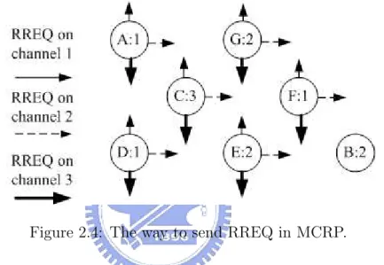
MCRP is modified from traditional AODV, and the procedure of route dis-covery is as follows. At the beginning, each node has assigned an random initial channel as shown in Figure 2.3. Assuming the number of non-overlapping channels is 3 (such as 802.11b), if node A wants to communicate with node B, A will send RREQ on all channels and intermediate nodes also rebroadcast it on all channels, as shown in Figure 2.4.
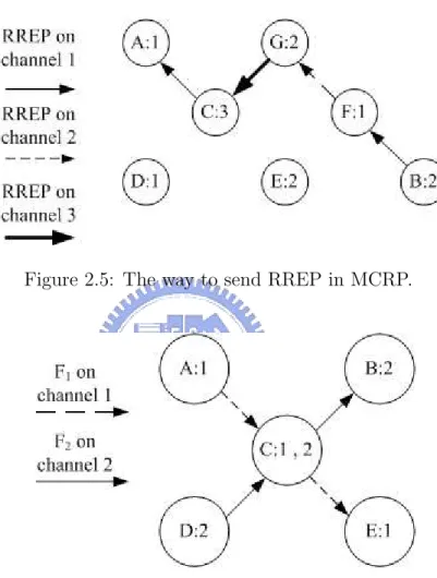
RREQ is modified from AODV by adding extra fields to gather nodes’ chan-nel information on a path. After destination node B receives a RREQ packet, it assigns a channel for this traffic flow and adds this assigned channel information in RREP packet. Then B sends RREP back to A using the reverse path to notify all intermediate nodes on the path their new channel. Not as RREQ, those RREP packets can be sent back on the channel which is recorded in RREQ before, as showed in Figure 2.5.
After that, all nodes on the routing path tune to the new channel to set up this traffic flow. Because nodes on the same traffic flow all stay on the same channel, they won’t have the deafness problem. However, if two traffic flows with different channels intersect on the same node, the deafness problem will happen again, as shown in Figure 2.6.
Figure 2.3: The initial random channel assignment in MCRP.
Figure 2.4: The way to send RREQ in MCRP.
There are two traffic flows F1 and F2. F1 is from A to E using channel 1; F2
is from D to B using channel 2. F1 and F2 intersect on node C. Because C is
as-signed multiple channels, we call C a switching node. When C communicates with E on channel 1, C can’t hear the message from D on channel 2 at the same time. Therefore, the deafness problem will happen again. For avoiding this problem, authors let each switching node send Join and Leave message to notify neighbors its operating channel before switching channels. Join message means to enter this channel; Leave message refers to leave this channel.
to tune to channel 2, it will send Leave message on channel 1 to notify neighbors that it will leave this channel, and then switch to channel 2 to send Join message to notify neighbors that it is on this channel now, as shown in Figure 2.7.
Figure 2.5: The way to send RREP in MCRP.
Figure 2.6: Node C has the deafness problem.
Therefore, A and E won’t send data to C to avoid the problem; D and B both know they can communicate with C. If C wants to tune to channel 1 again, it will also send Leave message on channel 2, and then send Join message on channel 1, as shown in Figure 2.8. As a result, B and D won’t send data to C to avoid the deafness problem; A and E also know they can communicate with C now.
However, this method can’t solve the deafness problem when there are two consecutive switching nodes, as shown in Figure 2.9.
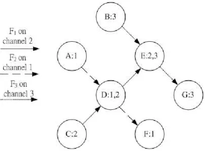
In Figure 2.9, there are three traffic flows F1, F2 and F3. F1 is from C to
E on channel 2; F2 is from A to F on channel 1; F3 is from B to G on channel
3. E and D are two consecutive switching nodes. For example, assuming E is on channel 2 first. When E wants to change channel from 2 to 3, E will send Leave message on channel 2, and then send Join message on channel 3 to its neighbors. But one of E’s neighbors (D) is also a switching node; it may not stay on channel 2 to hear this Leave message at time. Therefore, D may send data to E, when E is not on channel 2 which causes the deafness problem. Authors avoid the deafness problem in this situation by avoiding two consecutive switching nodes on traf-fic flows. For this reason, Authors design a channel table to gather the channel information of all nodes on the traffic flow from source to the destination. The channel table is added in RREQ. After nodes receiving RREQ, they update the channel table according to its own channel information, and then rebroadcast it. When destination node receives RREQ, it can choose a channel for this traffic flow by using the channel information without causing two consecutive switching nodes.
2.4
Disadvantages of MCRP
Although the previous work MCRP can avoid the deafness problem in MCSR environment, this method still has some disadvantages. First, the method of MCRP to avoid two adjacent nodes will cause over-count problem. That means
they also discard some routing paths without the deafness problem. We will dis-cuss it in the next chapter. Second, assigning only one channel on the traffic flow is not a good idea. Because different parts of the routing path may have differ-ent interferences levels on the same channel, choosing only one channel may cause some parts of the traffic flow with the high co-channel interference. Third, they won’t allow to assign more than two channels on a node. This restriction may also discard some routing paths without the deafness problem. When the number of traffic flows becomes larger, finding a new routing path without deafness problems becomes harder. It is possible that we can’t find any routing path without the deafness problem, but it truly exists.
Regardless those shortcomings, MCRP still has a good performance than traditional routing protocol (ex.AODV). And it is also an easy way to solve the deafness problems in dynamic channel assignment without time synchronization method. Therefore, in the next chapter, we will propose our enhanced methods which are based on MCRP without those weaknesses in MCSR environment to solve the deafness problem.
Figure 2.8: Switching node C changes its channel from 2 to 1.
Chapter 3
Modified-MCRP
In this chapter, first, we show how MCRP does to avoid the deafness prob-lem in detail. And then, we propose our Enhanced-MCRP (one-channel version) to find all feasible channel assignments on the path. Finally, we propose our Split Enhanced-MCRP (two-channels version) to find all feasible channel assignments on the path.
3.1
MCRP
3.1.1
Node Classification
In MCRP, nodes can be classified into 4 states.
1. Free node: A node has no traffic flows on it, and it is free to assign any channel.
2. Locked node: A node has a traffic flow with a certain channel on it.
3. Switching node: A node is assigned multiple channels (at most 2)for different traffic flows on it.
4. Hard-locked node: A node has a traffic flow with a certain channel on it. Because it is a adjacent node of a switching node, it can’t be assigned multiple channels to become a switching node.
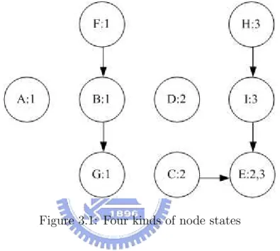
For example, in Figure 3.1, A and D are free nodes; B, F, G and H are locked nodes; E is a switching node; C and I are both hard-locked nodes.
Figure 3.1: Four kinds of node states
3.1.2
Gather Channel Usage Information in Each Node’s
Neighborhood
MCRP lets each node to set up its own flow table to maintain traffic flow information on all channels in its neighborhood. The traffic flow information can be seen as the number of flows on each channel to represent the channel usage in its neighborhood as shown in Figure 3.2. Fi is the load of channel i in its
neigh-borhood. And each node sets up its own flow table as follows.
F
1 F2 ... Fk
Figure 3.2: Flow table in each node
2. Hello messages contain the number of traffic flows through a node on each channel.
3. After receiving Hello messages, each node builds up its own flow table, ac-cording to the number of flows on each channel in the Hello messages from its neighbors and itself.
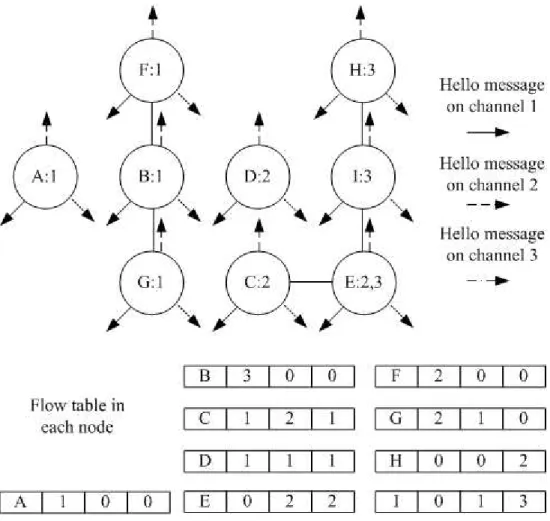
For example, in Figure 3.1, each node can finally set up its own flow table, as shown in figure 3.3.
Take node D for instance, D can receive the Hello message from B, C and I. Therefore, D knows B has one flow on channel 1; C has one flow on channel 2; I has one flow on channel 3; and D itself has no traffic flow. Finally, D can set up its flow table (1,1,1) as shown in Figure 3.3.
3.1.3
Route Discovery
When a node wants to communicate with another node, it will send RREQ and intermediate nodes also rebroadcast it until the destination node receives. Channel table and flow table are added in RREQ to gather all nodes information on the path from source to destination. The channel table is used for destination to determine which channel can be assigned without the deafness problem, and the flow table is used to assign the lowest load channel from those feasible channels on the path. The channel table and the flow table in RREQ contain a field for each
channel as shown in Figure 3.4 and Figure 3.2.
Figure 3.3: Each node sets up its own flow table
C
1 C2 ... Ck
Figure 3.4: Channel table in RREQ
After a node receives RREQ, it will update the channel table in the RREQ. The way to update the channel table is depended on different nodes’ states as follows.
1. Free node: Do nothing.
2. Locked node: If the assigned channel is channel i, add 1 on chi.
3. Switching node: If the two assigned channels are channel i and j, add 1 on both chi and chj
4. Hard-locked node: If the assigned channel is channel i, add 2 in chi.
After updating the channel table, node i also updates the flow table. The way to update the flow table in RREQ is as follows. For each channel c, if Fc(i) > Fc,
then update Fc to Fc(i). Fc(i) is the cth field of node i’s flow table; Fc is the cth
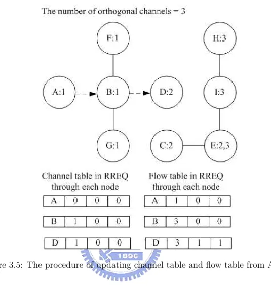
field of RREQ’s flow table. The idea to update the flow table is to record the highest number of flows on each channel along the routing path. For example, in Figure 3.3, if node A wants communicate with D, A will update and send RREQ. After B receives RREQ, B also updates and rebroadcasts it. After destination node D receives the RREQ from B and updates it, we can see channel table and flow table in RREQ, as shown in Figure 3.5
In Figure 3.5, according to Figure 3.3, because node A is a free node and
F1(A) > F1, A does nothing in the channel table (0,0,0) and updates the flow
table to be (1,0,0). Because node B is a locked node on channel 1 and F1(B) > F1,
B updates the channel table to be (1,0,0) ; updates the flow table to be (3,0,0). Because D is a free node, F2(D) > F2 and F3(D) > F3, D does nothing in the
channel table (1,0,0) and updates the flow table to be (3,1,1).
After the destination node receives and updates the channel table and the flow table in RREQ, it will determine if there is a feasible channel without causing
Figure 3.5: The procedure of updating channel table and flow table from A to D two adjacent switching nodes or not by checking the channel table in RREQ in the following rules.
1. Multiple channels have values grater than or equal to 2. 2. More than two channels have values grater than or equal to 1.
If one of those conditions matches, then the route has no feasible channels to assign, and then drops the RREQ. Otherwise, the route is feasible and the des-tination node will choose a channel considering the flow table in RREQ, according to following rules.
1. If a channel in the channel table has a value grater than or equal to 2, this channel has to be selected.
2. If two channels in the channel table have a value 1, then one of these two channels which has the lower traffic load in the flow table is selected.
3. If only one channel in the channel table has a value 1 and all other channels have 0, then among all channels, a channel with the minimum traffic load in the flow table is selected.
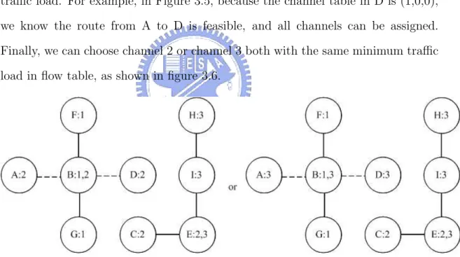
As a result, we use the flow table to choose a feasible channel with the lowest traffic load. For example, in Figure 3.5, because the channel table in D is (1,0,0), we know the route from A to D is feasible, and all channels can be assigned. Finally, we can choose channel 2 or channel 3 both with the same minimum traffic load in flow table, as shown in figure 3.6.
Figure 3.6: Traffic flow from A to D can assign channel 2 or channel 3 For increasing the routing path candidates, destination node can delay a pe-riod of time to send RREP back to the source node after receiving the first RREQ. During this time period, destination node can receive many RREQ messages from
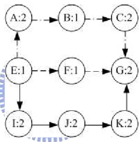
different nodes as shown in Figure 3.7, and then record the best one. After this time period, destination node will send the RREP back to the best routing path.
In Figure 3.7, source node E wants to communicate with destination node G. After destination node G receives the first RREQ from node F. It will delay a time preiod to receives more RREQ messages. After a time period, G will receive the RREQ from node C, F and K. Then it can choose the lowest load routing path, and send RREP back.
Figure 3.7: Destination node G can choose one of the routing paths with the lowest interference one
3.2
Enhanced MCRP (EMCRP)
In the pervious section, we show how MCRP works to avoid two adjacent switching nodes. Unfortunately, besides discarding infeasible channels, they also discard some feasible channels without the deafness problem. For example, in Fig-ure 3.8, although the dotted traffic flow from A to E can assign channel 3 without two adjacent nodes, there are more than 2 fields in the channel table with the value
grater than or equal to 1. Therefore, MCRP can’t find it and cause no feasible channels on the path. Finally, the path will be seen as an infeasible routing path. If there are already many flows in the network, it is hard to find a feasible path for new traffic demands. It is not a good idea to discard any feasible channels. Besides, it is possible to discard routing paths with lower traffic load. Therefore, we design a method to find all feasible channels as follows.
Figure 3.8: MCRP discards the feasible channel 3
3.2.1
Node Classification
First, because MCRP can only assign two channels on switching nodes, it also discards some feasible channels which cause switching nodes with more than 2 channels. For finding these feasible channels, we can set the upper bound of the
number of channels which can be assigned on switching nodes. If the number of channels on a switching node is lower than the upper bound, we can still assign more channels on it. Therefore, we classify switching nodes again into two parts as follows.
1. Switching node (A): A node has multiple traffic flows on different channels through it, and the number of channels is below the upper bound which means it can still assign a new channel.
2. Switching node (B): A node has multiple traffic flows on different channels through it, and the number of channels is equal to the upper bound which means it can’t assign a new channel any more.
3.2.2
Route Discovery
Second, as MCRP, we also add channel table and flow table in RREQ. The flow table is the same as MCRP, but the channel table is the totally different meaning. The channel table contains a field for each channel as shown in Figure 3.4, but the value of each field is 0 or 1. 0 means the channel is infeasible to assign; 1 means the channel is feasible to use.
Third, excepting channel table and flow table, we add the sender informa-tion which contains sender’s assigned channels and state informainforma-tion as shown in Figure 3.9.
The sender doesn’t mean the source node of the routing path. When a node broadcasts or rebroadcasts the RREQ, it is the sender of RREQ message. The
ch1
Sender channel information
S1
S2
S3
S4
Sender state information
S5
ch2
...
chk
Figure 3.9: Sender’s channel and state information
sender channel information records channels it has assigned. All fields in sender channel information are boolean. 1 means sender has assigned the channel, and 0 means sender has not assigned it. The sender state information records which state it is. S1 refers to free node, S2 refers to locked node, S3 refers to hard-locked node, S4 refers to switching (A) node, and S5 refers to switching (B) node. All fields in sender state information are also Boolean. 1 means sender is on this state, and 0 means not.
Forth, after receiving RREQ, nodes can update the channel table, the flow table and the sender information in RREQ. The way to update the flow table is the same as MCRP, but the way to update channel table is different from MCRP as follows. S is the sender of RREQ, R is the receiver of RREQ and C presents the channel table in RREQ. Source node needs to generate the channel table in RREQ, and intermediate nodes also have to update the channel table, according to Figure 3.10.
The main idea to update the channel table is to set all channels can be as-signed first, and then delete infeasible channels node by node. Infeasible channels are channels which will cause two adjacent switching nodes. After a node receives
RREQ, because we add the sender information in RREQ, it will have two adja-cent nodes information (sender and itself) to avoid two adjaadja-cent switching nodes causing infeasible channels. Finally, destination node can choose the lowest load channel from those feasible channels by using the same way as shown in MCRP.
For example, we use our extended method on the same traffic flow in Figure 3.8. And we can find a feasible channel as shown in Figure 3.11
According to Figure 3.10, node A is a free node, and it is also a source node. Therefore, it sets up the channel table to be (1,1,1). After B receives RREQ, it knows sender A is free, and receiver B is a locked node , then updates the channel table to be (1,1,1). After C receives RREQ, it knows sender B is a locked node on channel 1, and receiver C is a locked node on channel 3, then updates the channel table to be (1,0,1). After D receives RREQ, it knows sender C is a locked node on channel 3, and receiver D is a locked node on channel 2, then updates the channel table to be (0,0,1). After E receives RREQ, it knows sender D is a locked node on channel 2, and receiver E is a free node, then updates the channel table to be (0,0,1). Because the field of channel 3 in the channel table is one, node E can assign channel 3 on the routing path without the deafness problem as shown in Figure 3.12.
3.3
Split Enhanced MCRP (SEMCRP)
There are two advantages of having the possibility to assign multiple channels on the routing path. We show the details as follows.
First, it may decrease the bottleneck channel load on the path. In MCRP, destination node can only assign one channel on the traffic flow. But when the routing path is long, different parts of the path may have different traffic load on the same channel. It is not a good idea to assign only one channel on the routing path. Therefore, assigning multiple channels according to different traffic load in-formation each node can decrease bottleneck channel load on the path.
For example, in Figure 3.13, the dotted line is a candidate routing path from F to J. Because MCRP and EMCRP can only assign one channel on the routing path, it can assign channel 1, 2 or 3 all with the same bottleneck channel load 1. But if we use SEMCRP to assign channels as shown in Figure 3.14, we can assign channel 3 from F to H, and channel 1 from H to J with the bottleneck channel load 0. Therefore, SEMCRP can assign multiple channels to decrease the bottleneck channel load for increasing throughput.
Second, it can find more feasible channel assignments. In some situations, assigning one channel on the routing path can’t find any feasible channels as shown in Figure 3.15. After destination node F receives RREQ and updates it, F finds the channel table which has more than 2 fields with value grater than or equal to 1. Therefore, there are no feasible channels in MCRP.
But, if we assign multiple channels on the routing path, there are still some feasible channels which can be assigned as shown in Figure 3.16. We can assign channel 2 from A to D, and assign channel 3 from D to F. And there are no two
adjacent switching nodes after this channel assignment.
As a result, we design a Split Enhanced MCRP to split the routing flow into two parts, and find all feasible channels to assign on each part without causing two adjacent switching nodes.
3.3.1
Route Discovery
In SEMCRP, we also classify the switching nodes into two types as shown in EMCRP. For assigning multiple channels on the path, We need to gather more information for destination to assign multiple channels without the deafness prob-lem. Without adding channel table and flow table in RREQ, RREQ needs to add each node’s channel information (C[A][B]), flow information (f [A][B]) and state information (S[A][B]) on the path as shown in Figure 3.17. C[A][B] and f [A][B] are both n × M matrixes; S[A][B] is a n × 5 matrix. n is the number of nodes on the path, and M is the number of orthogonal channels. C[A][B] = 1 means that node A is assigned channel B, f [A][[B] is the number of traffic flows on channel B in node A’s neighborhood. S[A][B] = 1 means node A’s state is B.
In Figure 3.17, when A sends RREQ, it appends its channel, state and flow information in RREQ. After B receives RREQ, it also appends its channel, state and flow information in the RREQ. Finally, destination node F can gather all nodes information on the routing path.
table (F [A][B]) and rear table (R[A][B]) by using channel and state information in RREQ. Front table can figure out feasible channels on the path from source node to intermediate nodes. The way to set up front table is the same as to set up channel table in RREQ from source to destination as EMCRP. The procedure is shown in Figure 3.18.
We set up the front table by checking nodes information from source to destination in RREQ. We modify Figure 3.10 to Figure 3.20 which is suitable for setting the front table. According to Figure 3.20, because A is the source node, and the state is free, it can assign all channels to be 1 on its fields in the front table. And receiver node B is a locked node on channel 1; sender A is a free node, B can assign all channels to be 1 on its fields in the front table. After the last field is established in the front table, the front table is completed.
Rear table can figure out the feasible channels on the path from destination node to intermediate nodes. The way to set up rear table is the same as to set up front table with different direction from destination to source. The procedure is shown in Figure 3.19.
We set up the rear table by checking nodes information in different direction from destination to source in RREQ. We also modify Figure 3.10 to Figure 3.21 which is suitable for setting the rear table. Assume there is another traffic flow k from F to A on the same dotted path. According to Figure 3.21, because F is a source node in traffic flow k, and the state is free, it can assign all channels to be 1 on its fields in the rear able. And receiver E is a hard-locked node on channel 3;
sender F is a free node. Therefore, E can assign channel 3 to be 1 on its fields in the rear table. After the first field is set up in the rear table, the rear table is completed.
After creating front table and rear table, we can set up front split table by using front table; set up rear split table by using rear table. Front split table (FS[A][B]) and rear split table (RS[A][B]) are both n − 2 × M matrixes as shown in Figure 3.22.
Front split table is to determine which node can be a split node without causing two adjacent switching nodes in the first part of the routing path. A split node means a node will be a switching node, and splits the routing path into two parts. The first part is assigned one channel, and the second part is assigned an-other. F S[A][B] = 1 means node A can be a split node when the first part of the routing path is assigned channel B. Rear split table is to determine which node can be a split node without causing two adjacent switching nodes in the second part of the routing path. RS[A][B] = 1 means node A can be a split node when the second part of the routing path is assigned channel B. If node A can be a split node in both front split table and rear split table, the routing path can be assigned one channel from source to A, and another from A to destination without deafness problems as shown in Figure 3.16. The way to set up front split table is as follows.
1. A routing path can only be split from node 2th to node n-1th, we only consider those nodes.
those either.
3. If F [A][B] == 1 and node A-1th is a free or hard-locked node, then F S[A][B] = 1
4. If F [A][B] == 1 and node A-1th is a locked node and C[A − 1][B] == 1, then F S[A][B] = 1
Therefore, we can set up the front split table by using the front table in Figure 3.18 and node information in Figure 3.17, as shown in Figure 3.23
The way to set up the rear split table is as follows
1. A routing path can only be split from node 2th to node n-1th, we only consider those nodes.
2. Hard-locked nodes can’t be assigned more than 2 channels, we don’t consider them either.
3. If R[A][B] = 1 and node A+1th is a free or hard-locked node, then RS[A][B] = 1
4. If R[A][B] = 1 and node A+1th is a locked node and C[A + 1][B] == 1, then
RS[A][B] = 1
Therefore, we can use the rear table in Figure 3.19 and node information in Figure 3.17 to set up the rear split table as shown in Figure 3.24.
Finally, according to those two split tables, if node A exists a channel C and a channel B, lets F S[A][B] == 1 and RS[A][C] == 1, B 6= C, then the first part of the path can be assigned channel B from source to A, and the second part can be assigned channel C from A to destination. For example, because F S[C][1] == 1 in Figure 3.23 and RS[C][3] == 1 in Figure 3.24, C can be the split node. The first part of the path can be assigned channel 1 from source to C, and the second part can be assigned channel 3 from C to destination, as shown in Figure 3.25.
Furthermore, F S[D][2] and RS[D][3] are equal to 1, D can also be a split node. The first part of the path can be assigned channel 2 from source to D, and the second part of the path can be assigned channel 3 from D to destination, as shown in Figure 3.26.
As we can see, there are two feasible channel assignments in Figure 3.25 and Figure 3.26. We choose the assignment with the lowest bottleneck channel load. The bottleneck channel load is the highest channel load on the routing path after channel assignment. In Figure 3.27, destination node F can use the flow information table in RREQ to find the bottleneck load for each assignment. The way to find the bottleneck load is the same as MCRP which records the highest number of traffic flow on assigned channels along the path. After checking the flow information, the bottleneck load in Figure 3.25 and 3.26 are the same. Therefore, we can choose any of those two assignments for the routing path.
Besides, before we create rear table to assign multiple channels on the rout-ing path, we can also use front table to find the feasible channels for the routrout-ing
path without splitting it. If F [D][B] = 1, D is the destination node, then chan-nel B can be assigned on the routing path. Therefore, we can choose a chanchan-nel assignment with the lowest bottleneck load from one channel and two-channel as-signments.
As a result, our Split Enhanced MCRP can not only find more feasible chan-nels than MCRP, but also assign different chanchan-nels on each part to decrease the bottleneck channel load. In the next chapter, we will show our extend MCRP methods cause better performance in different simulations.
Source node Free Locked Hard-locked Switching(A) Switching(B) Channel table All channels = 1 All channels = 1 Assigned channel = 1 All channels = 1 Assigned channels = 1 Generate channel table
Update channel table R(Receiver) Free Locked Hard-locked Switching(A) Switching(B) Channel table C = C C = C
C = C joint the channel of R C = C
C = C joint the channels of R S(Sender) Free or Hard-locked R(Receiver) Free Locked Hard-locked Switching(A) Switching(B) Channel table C = C
C = C joint (the channel of S
union the channel of R ) C = C joint the channel of R
C = C
C = C joint the channels of R S(Sender) Locked R(Receiver) Free Locked Hard-locked Switching(A) Switching(B) Channel table C = C
C = C joint the channel of R C = C joint the channel of R Empty
Empty S(Sender)
Switching (A) or (B)
(C is the channel table in RREQ)
Figure 3.11: EMCRP updates channel table from source to destination
Figure 3.12: The dotted traffic flow can be assigned channel 3 without the deafness problem
Figure 3.13: MCRP or EMCRP can assign all channels with the same bottleneck channel load 1
Figure 3.14: SEMCRP can assign channel 3 from F to H, and channel 1 from H to J with the bottleneck channel load 0
Figure 3.16: Split Enhanced MCRP can find a feasible channel assignment on the routing path
Figure 3.17: Destination F will have channel, flow and state information of all nodes on the routing path
Ch A 1 1 2 1 3 1 Ch A 1 1 2 1 3 1 Ch A 1 1 2 1 3 1 B 1 1 1 B 1 1 1 C 1 1 0 Ch A 1 1 2 1 3 1 B 1 1 1 C 1 1 0 D 1 1 0 Ch A 1 1 2 1 3 1 B 1 1 1 C 1 1 0 D 1 1 0 E 0 0 0 Ch A 1 1 2 1 3 1 B 1 1 1 C 1 1 0 D 1 1 0 E 0 0 0 F 0 0 0
Figure 3.18: Destination node F sets up the front table
Ch F 1 1 2 1 3 1 Ch E 1 0 2 0 3 1 Ch D 1 0 2 0 3 1 F 1 1 1 E 0 0 1 F 1 1 1 Ch C 1 0 2 0 3 1 D 0 0 1 E 0 0 1 F 1 1 1 Ch B 1 0 2 0 3 0 C 0 0 1 D 0 0 1 E 0 0 1 F 1 1 1 Ch A 1 0 2 0 3 0 B 0 0 0 C 0 0 1 D 0 0 1 E 0 0 1 F 1 1 1
Source node Free Locked Hard-locked Switching(A) Switching(B) Front table
All channels = 1 on the first field
Only assigned channel = 1 on the first field All channels = 1 on the first field
Only assigned channels = 1 on the first field Generate front table
Update front table
R(Receiver) Free Locked Hard-locked Switching(A) Switching(B) Front table F[R] = F[S] F[R] = F[S]
F[R] = F[S] joint the channel of R F[R] = F[S]
F[R] = F[S] joint the channels of R S(Sender) Free or Hard-locked R(Receiver) Free Locked Hard-locked Switching(A) Switching(B) Front table F[R] = F[S]
F[R] = F[S] joint (the channel of S
union the channel of R ) F[R] = F[S] joint the channel of R
F[R] = F[S]
F[R] = F[S] joint the channels of R S(Sender) Locked R(Receiver) Free Locked Hard-locked Switching(A) Switching(B) Front table F[R] = F[S]
F[R] = F[S] joint the channel of R F[R] = F[S] joint the channel of R Empty
Empty S(Sender)
Switching (A) or (B)
( F[S] means fields on sender node in the front table ) ( F[R] means fields on receiver
node in the front table )
Source node Free Locked Hard-locked Switching(A) Switching(B) Rear table
All channels = 1 on the first field
Only assigned channel = 1 on the first field All channels = 1 on the first field
Only assigned channels = 1 on the first field Generate rear table
Update rear table
R(Receiver) Free Locked Hard-locked Switching(A) Switching(B) Rear table R[r] = R[s] R[r] = R[s]
R[r] = R[s] joint the channel of R R[r] = R[s]
R[r] = R[s] joint the channels of R S(Sender) Free or Hard-locked R(Receiver) Free Locked Hard-locked Switching(A) Switching(B) Rear table R[r] = R[s]
R[r] = R[s] joint (the channel of S
union the channel of R ) R[r] = R[s] joint the channel of R
R[r] = R[s]
R[r] = R[s] joint the channels of R S(Sender) Locked R(Receiver) Free Locked Hard-locked Switching(A) Switching(B) Rear table R[r] = R[s]
R[r] = R[s] joint the channel of R R[r] = R[s] joint the channel of R Empty
Empty S(Sender)
Switching (A) or (B)
( R[s] means fields on sender node in the rear table ) ( R[r] means fields on receiver
node in the rear table )
Figure 3.22: Front split table and rear split table Ch B 1 1 2 1 3 1 C 1 0 0 D 0 1 0 E 0 0 0
Figure 3.23: Destination node F sets up the front split table
Ch B 1 0 2 0 3 0 C 0 0 1 D 0 0 1 E 0 0 0
Figure 3.24: Destination node F sets up the rear split table
Figure 3.25: The routing path is from A to F,A to C is on channel 1; C to F is on channel 3
Figure 3.26: The routing path is from A to F, A to D is on channel 2; D to F is on channel 3
Chapter 4
Simulation
In this chapter, we use the ns-2 simulator to evaluate the performance of our enhanced MCRP methods, original MCRP and traditional AODV. We measure the throughput in the network with traffic flows to be our performance metric. At first, we evaluate the network throughput in different number of traffic flows. And then, we figure out the throughput in different traffic rate. The traffic flow is the pair of the source node and the destination node. We randomly generate several sets of traffic flows to find the average throughput in different number of traffic flows and in different traffic rate. Finally, we will show our methods which can have the better performance than original MCRP and AODV.
Each node is fixed in the network. The transmission range of each node is approximately 20m, and the IEEE 802.11 DCF is used as the MAC protocol. The number of orthogonal channels is 3 and the maximum bandwidth on each channel is 11 Mbps, such as 802.11b. And we set the maximum number of channels which can be assigned on a node is 2. For the traffic flow, we use the constant bit rate traffic with the packet size 512 bytes. When a node is a switching node, it needs to switch its operating channel every 50ms.
In the first simulation, we want to figure out the average network through-put with varying the number of traffic flows (5, 10, 15, 20, 25, 30). There are 100 nodes in the network, and the network topology is grid, as shown in Figure 4.1. Each traffic flow has the bit rate 4Mbps, and we add it one by one every 10 sec in the network. With this high transmission rate, the channel bandwidth will be saturated when the number of flows increases. The result is shown in Figure 4.3. There are four methods AODV, MCRP, Enhanced MCRP(EMCRP), and Split Enhanced MCRP(SEMCRP). When the number of traffic flows increases, the throughput decreases gradually. Because AODV only has one single channel to use, the performance is the worst one. MCRP, EMCRP and SEMCRP all have multiple channels to use, therefore they can improve the throughput largely. Fur-thermore, EMCRP have the better performance than MCRP, because it doesn’t discard any feasible routing paths. When the traffic load is high, SEMCRP can has a better performance than EMCRP, because it can assign a path with at most 2 channels to decrease the load of bottleneck channel. A path with the lower bot-tleneck channel load can help to increase throughput.
In the second simulation, we want to determine the average network through-put with different the traffic rates. We vary the traffic rates (32Kbps, 64Kbps, 128Kbps, 256Kbps, 512Kbps, 1024Kbps, 2048Kbps, 4096Kbps) with 15 traffic flows. There are 49 nodes in the network, and the network topology is also grid, as shown in Figure 4.2. The result is shown in Figure 4.4. We can see MCRP, EMCRP and SEMCRP all have higher throughput than AODV. When the traffic rate is low, all methods almost have the same performance, because channels are
Figure 4.1: 100 nodes grid topology
still not saturated. Because EMCRP and SEMCRP can choose the routing path without discarding any feasible ones, they have more chances to choose the path with lower bottleneck channel load than MCRP. As a result, when the traffic rate is high, choosing the path with the lower bottleneck channel load can help to in-crease throughput largely. Besides, SEMCRP is also better than EMCRP when the traffic rate is high, because it can assign multiple channels on a routing path to decrease the load of bottleneck channel on the routing path.
In the third simulation, we want to know the route discovery overhead be-tween MCRP, EMCRP and SEMCRP with different number of traffic flows (5, 10, 15, 20, 25, 30). We use the control packet RREQ and RREP to be the route discovery overhead. The network topology is the same with the first simulation, as shown in Figure 4.1. Each traffic flow has the bit rate 4Mbps, and we add it one by one every 10 sec in the network. The result is shown in Figure 4.5. The
route discovery overhead is SEMCRP > EMCRP > MCRP. Because the packet size of RREQ and RREP in MCRP is the smallest one, it has the lowest overhead than others. In SEMCRP, for gathering all nodes information on the path, it has the largest control packet RREQ causing the highest overhead. When the number of traffic flows increases in the network, the route discovery becomes harder and harder. As a result, when the number of traffic flows is higher, the difference of overhead between SEMCRP and MCRP is larger.
According to Figure 4.3 and 4.4, the simulation result shows our EMCRP and SEMCRP both have a better performance than MCRP when the traffic load is heavy. And SEMCRP also has a better throughput than EMCRP when the traffic load is high. In Figure 4.5, because of the largest RREQ in SEMCRP, SEMCRP has the highest route discovery overhead than others.
0 5 10 15 20 25 30 35 0 0.5 1 1.5 2 2.5 3 3.5 4
Number of traffic flows
Network throughput (Mbps)
AODV MCRP EMCRP SEMCRP
Figure 4.3: Network throughput with different number of flows
0 500 1000 1500 2000 2500 3000 3500 4000 4500 0 1 2 3 4 5 6 Traffic rate (Kbps) Network throughput (Mbps) AODV MCRP EMCRP SEMCRP
0 5 10 15 20 25 30 35 0 500 1000 1500 2000 2500 3000 3500 4000
Number of traffic flows
Cumulative route discovery overhead (KB)
MCRP EMCRP SEMCRP
Chapter 5
Conclusion and Future Work
In this thesis, we propose EMCRP and SEMCRP methods to overcome short-ages of MCRP. In EMCRP, we can choose a routing path without ignoring any feasible candidates. In SEMCRP, we can not only choose a routing path with-out discarding any feasible paths, but also have the ability to assign at most two channels on a path to reduce the interference. Because the channel usage may be different from source to destination in a long routing path, SEMCRP can assign multiple channels, according to different parts of the routing path. In the simula-tion result, we learn that both EMCRP and SEMCRP have the better performance than MCRP when the traffic load is heavy.
However, the MCRP and our proposed methods still have some issues to address. First, switching nodes can only stay on each channel with the same time period. Staying on each channel with the same time period is not a good idea. Switching nodes should decide how long it can stay on each channel, according to the traffic flows through it. That is when the packet queue on a certain channel is high, it should stay on that channel for a long time.
Second, in MCRP, each node has only one antenna which means they can’t transmit and receive at the same time. But in multi-radio environment, nodes can use multi-radio to increase throughput which has a higher performance than MCRP. Therefore, modifying MCRP to be suitable in multi-radio environment could be an important issue.
Third, in SEMCRP, our method can only assign at most two channels on the routing path to decrease the bottleneck channel load without causing deaf-ness problems. However, assigning more than two channels on the path may have higher possibility to find channel assignments with lower co-channel interference than two-channel SEMCRP. As a result, modifying SEMCRP with the ability to assign more than 2 channels is a worth thing to do.
Finally, in SEMCRP, the size of RREQ is large. That is the overhead of route is high. The high route discovery overhead will decrease the network band-width. Therefore, finding an efficient way to gather nodes information on the path is also a possible future work.
Bibliography
[1] X.H. Lin, Y.K. Kwok and V.K.N. Lau, ”On Channel-Adaptive Routing in an IEEE 802.11b Based Ad Hoc Wireless Networks”, Proc. IEEE GLOBECOM, pp.3509-3513, 2003
[2] Y. Seok, J. Park and Y. Choi, ”Multi-rate Aware Routing Protocol for Mobile Ad Hoc Networks”, Proc. IEEE Vehicular Technology Conference, pp.1749-1752, 2003
[3] D.S.J.D. Couto, D. Aguayo, J. Bicket and R. Morris, ”A High-Throughput Path Metric for Multi-Hop Wireless Routing”, Proc. ACM MobiCom, pp.134-146, 2003
[4] S. Biswas and R. Morris, ”ExOR: Opportunistic Multi-Hop Routing for Wire-less Networks”, Proc. ACM SIGCOMM, pp.133-143, 2005
[5] R. Draves, J. Padhye and B. Zill, ”Comparison of Routing Metrics for Static Multi-Hop Wireless Networks”, Proc. ACM SIGCOMM, Volume 34 Issue 4, 2004
[6] L. lannon´e and S. Fdida, ”MRS: A Simple Cross-Layer Heuristic to Improve
Throughput Capacity in Wireless Mesh Networks”, Proc. ACM CoNEXT, pp. 21-30, 2005
[7] R. Draves, J. Padhye and B. Zill, ”Routing in Multi-Radio, Multi-Hop Wire-less Mesh Networks”, Proc. ACM MobiCom, pp.114-128, 2004
[8] V.S.A. Kumar, M.V. Marathe and Srinivasan, ”Algorithmic Aspects of Ca-pacity in Wireless Networks”, Proc. ACM SIGMETRICS, pp.133-144, 2004 [9] K.Jain, J. Padhye, V. Padmanabhan and L. Qiu, ”Impact of Interference on
Multi-Hop Wireless Network Performance”, Proc. ACM MobiCom, 2003 [10] P. Bahl, R. Chandra and J. Dunagan, ”SSCH: Slotted Seeded Channel
Hop-ping for Capacity Improvement in IEEE 802.11 Ad-Hoc Wireless Networks”,
Proc. ACM MobiCom, pp.216-230, 2004
[11] J. So and N.H. Vaidya, ”A Multi-channel MAC Protocol for Ad Hoc Wireless Neworks”, Proc. ACM MobiHoc, 2003
[12] J. So and N. Vaidya, ”A Routing Protocol for Utilizing Multiple Channels in Multi-Hop Wireless Networks with a Single Transceiver”, UIUC Technical