Modeling Salt Water Intrusion in Tanshui River Estuarine
System—Case-Study Contrasting Now and Then
Wen-Cheng Liu
1; Ming-Hsi Hsu
2; Chi-Ray Wu
3; Chi-Fang Wang
4; and Albert Y. Kuo, M.ASCE
5Abstract: A vertical共laterally integrated兲 two-dimensional numerical model was applied to study the salt water intrusion in the Tanshui River estuarine system, Taiwan. The river system has experienced dramatic changes in the past half century because of human interven-tion. The construction of two reservoirs and water diversion in the upper reaches of the river system significantly reduces the freshwater inflow. The land subsidence within the Taipei basin and the enlargement of the river constriction at Kuan-Du have lowered the river bed. Both changes have contributed farther to the intrusion of tidal flow and salt water in the upstream direction. The model was reverified with the earliest available hydrographic data measured in 1977. The overall performance of the model is in reasonable agreement with the field data. The model was then used to investigate the change in salt water intrusion as a result of reservoir construction and bathymetric changes in the river system. The model simulation study reveals that significant salinity increases have resulted from the combined changes. It has been speculated by ecological researchers that the long-term increase in salinity might be the driving force altering the aquatic ecosystem structure in the lower reach of the estuary and the Kuan-Du mangrove swamp, particularly the enlargement of the mangrove area and the disappearance of freshwater marshes. However, concrete proof has not been available since no prototype salinity data were available prior to the reservoir construction. This case study offers the first quantitative estimate of the salinity changes due to human interference in this natural system.
DOI: 10.1061/共ASCE兲0733-9429共2004兲130:9共849兲
CE Database subject headings:Salt water intrusion; Taiwan; River systems; Numerical models; Reservoirs; Bathymetry.
Introduction
Throughout the history of civilization, mankind has tended to concentrate its activities along the courses of rivers. This has naturally led to the imposition of man-made changes on rivers, through the construction and operation of dams and reservoirs, river training and dredging, waste disposal, etc. An increasing number of diverse projects have required modifications to river systems, such as reservoir regulation or freshwater withdrawals. In these cases, upstream changes of the river runoff will inevita-bly have consequences on the estuarine portion of the river. Al-though river management has commonly occurred over the past 50 years, most studies have focused on the short or medium term
behavior of estuarine flows, few studies have been conducted and little is known about the long-term estuarine response associated with river management schemes共Kjerve 1976; Kjerfve and Greer 1978; McAlice and Jaeger 1983兲. For these reasons, there is a need for numerical modeling in conjunction with any estuary-related management plans. Numerical models have become im-portant tools to assess the response of natural systems to changes in environmental regulations and construction of engineering fa-cilities.
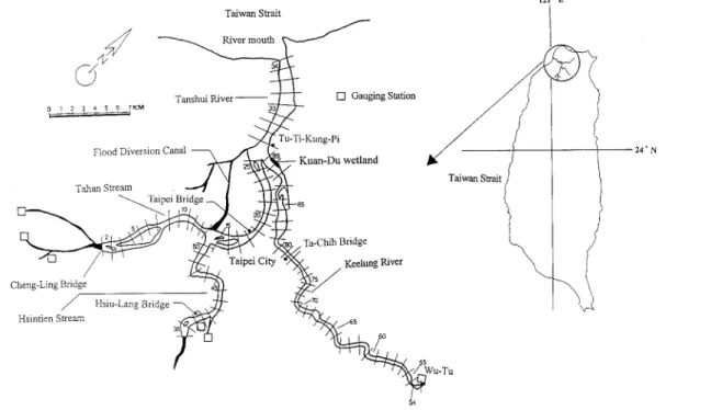
The Tanshui River estuary共Fig. 1兲 is the largest estuarine sys-tem in Taiwan, with its drainage basin including the capital city of Taipei. The tidal influence spans a total length of about 82 km, encompassing the entire length of the Tanshui River and the downstream reaches of its three major tributaries: the Tahan Stream, the Hsintien Stream, and the Keelung River. Except dur-ing the period of a flood event, the astronomical tide may reach as far upriver as Cheng-Ling Bridge in Tahan Stream, the Hsiu-Lang Bridge in Hsintien Stream, and the Chiang-Pei Bridge in Keelung River共Fig. 1兲. Tidal propagation is the dominant mechanism con-trolling the water surface elevation, and ebb and flood flows. The M2tide is the primary tidal constituent at the river mouth, with a tidal range of 2.17 m at mean tide, and up to 3 m at spring tide. Because of the cross-sectional contraction and wave reflection, the mean tidal range may reach a maximum of 2.39 m within the system. The phase relationship between tidal elevation and tidal flow is close to standing wave characteristics共Hsu et al. 1999a兲. Sea water intrudes upriver as a result of tidal advection and the classical two-layer estuarine circulation. Salinity varies in in-tratidal time scale in response to the ebb and flood of the flows as well as in various longer time scales in response to freshwater inflow. The limit of salt intrusion may reach beyond 25 km in the Tahan Stream from the river mouth during the period of low flow. 1Associate Professor, Dept. of Civil Engineering, National United
Univ., Miao-Li 360, Taiwan. E-mail: wcliu@hy.ntu.edu.tw
2Professor, Dept. of Bioenvironmental Systems Engineering and Senior Research Fellow, Hydrotech Research Institute, National Taiwan Univ., Taipei 10617, Taiwan 共corresponding author兲 E-mail: mhhsu@ccms.ntu.edu.tw
3Doctoral Student, Dept. of Bioenvironmental Systems Engineering, National Taiwan Univ., Taipei 10617, Taiwan.
4Doctoral Student, Dept. of Bioenvironmental Systems Engineering, National Taiwan Univ., Taipei 10617, Taiwan.
5Visiting Professor, Dept. of Bioenvironmental Systems Engineering and Senior Research Fellow, Hydrotech Research Institute, National Taiwan Univ., Taipei 10617, Taiwan.
Note. Discussion open until February 1, 2005. Separate discussions must be submitted for individual papers. To extend the closing date by one month, a written request must be filed with the ASCE Managing Editor. The manuscript for this paper was submitted for review and pos-sible publication on November 25, 2002; approved on February 10, 2004. This paper is part of the Journal of Hydraulic Engineering, Vol. 130, No. 9, September 1, 2004. ©ASCE, ISSN 0733-9429/2004/9-849– 859/$18.00.
The baroclinic pressure gradient set up by the salinity distribution is large enough to push the denser salt water upriver along the bottom layer of the estuary. This results in the classical two-layer circulation of net upriver flow in the bottom layer and net down-river flow in the upper layer 共Hsu et al. 1999a兲. The resulting estuarine circulation strengthens as the river flow decreases共Kuo and Liu 2001兲.
Two reservoirs, Feitsui Reservoir and Shihman Reservoir, were built in the upriver reaches of the Tanshui River system. Feitsui Reservoir, completed in 1987, had an initial design capac-ity of 406⫻106m3and was primarily designed to provide domes-tic water supply to the Taipei metropolitan area with a population over 5 million. The dam site of the Feitsui Reservoir is located at the lower end of the Peishih Stream, a tributary of the Hsintien Stream, and is about 30 km away from Taipei City. Shihmen Reservoir was completed in 1964 and situated at the upper end of the Tahan Stream. This multipurpose reservoir supplies water to the rice fields of northwest Taiwan and to Taipei during the dry season. Covering 8 km2, this man-made reservoir also generates 87,400 kW of electricity for the island’s insatiable demand. An-other vital function of these two reservoirs is to provide flood control in the typhoon season. Fig. 2共a兲 presents flow duration curves in the Tahan Stream before and after the Shihman Reser-voir construction. Fig. 2共b兲 shows flow duration curves in the Hsintien Stream before and after the Feitsui Reservoir construc-tion. These figures indicate that the river discharges have dramati-cally reduced after the reservoirs were constructed. As an ex-ample, the current Q50 flow is 50% less than that before the Shihman Reservoir construction.
The Taiwan Water Resources Agency has conducted regular bathymetric surveys of the river system since 1969. It measured the cross-sectional profiles of the river at about 0.5 km intervals along the tidal portion of the river. The survey results show con-siderable bathymetric change in the estuarine system. Fig. 3 com-pares the 1995, 1977, and 1969 river bed profiles, plotted along the river axis in the Tanshui River-Tahan Stream and Hsintien Stream. It shows that there has been extensive scouring along
Fig. 1. Map of Tanshui River system and model segments
Fig. 2. Comparison of flow duration curves before and after reser-voir construction in the共a兲 Tahan Stream and 共b兲 Hsintien Stream
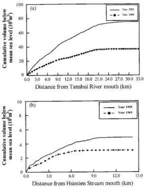
most of the river system, except for some local reaches. This results in a substantial increase in the cumulative volume below mean sea level for the entire estuarine system共Fig. 4兲.
Kuan-Du wetland is the largest estuarine wetland in the Tan-shui River system. It is situated on the northern shore of the Keelung River mouth共Fig. 1兲. It was reported that the vegetation types in the wetland had shifted from less salt-tolerant types to salt-tolerant types, namely mangroves. Using geographic infor-mation system and image processing techniques, Wang 共1999兲 interpreted a series of aerial photos from 1978 to 1997 to delin-eate the area extent of the three dominant types of vegetation in the wetland. He reported that the mangrove Kandelia candel had increased its aerial coverage from nearly 0 to 24 ha, about 68% of the total area. The less salt-tolerant Cyperus malaccensis de-creased from 10 ha in 1978 to none in 1997, while Phragmites communis decreased from about 20 to 10 ha. Wester共1988兲 sug-gested that the salinity increase in the river waters adjacent to the wetland might be the most important factor responsible for the continuing shift in vegetation type. Land subsidence was cited as the major culprit. It is expected that either of the two alternations of the river system described above will enhance the salt water intrusion into the system.
In this study, a vertical 共laterally integrated兲 two-dimensional hydrodynamic model was applied to study the Tanshui River es-tuarine system. The model had previously been calibrated and verified for the recent conditions of 1994 and 1995 共Hsu et al. 1999a兲. The model was further reverified with the earliest avail-able prototype data of 1977. The verified model was then used to simulate salt water intrusion under both the current conditions and the prereservoir conditions, respectively. The results show that the increase in salt water intrusion has the potential to favor the de-velopment of mangrove wetlands in the lower estuary near Kuan-Du.
Model Description
Many numerical models have been developed to simulate the hy-drodynamic behavior of estuaries using one-, two-, or three-dimensional frameworks. Although full three-three-dimensional models
共e.g., Casulli and Cheng 1992; Johnson et al. 1993; Wang et al.
1994; Blumberg et al. 1999; Lai et al. 2003兲 have increasingly been used, a two-dimensional laterally integrated model offers an efficient and practical tool for narrow and partially mixed estuar-ies. In a narrow channel with steep bathymetric variations, a suf-ficiently fine grid must be designed for a three-dimensional model to resolve the lateral bathymetric gradients. It is computationally intensive and often unnecessary since the dominant transport mechanisms and their variations are in the longitudinal and ver-tical directions.
A laterally integrated two-dimensional, real-time model of hy-drodynamics and salinity was developed for application to the tidal portion of the Tanshui River estuarine system 共Hsu et al. 1996, 1997兲. The model is actually quasi-three-dimensional, since it also includes the simulation of shoals and shallow embayments adjacent to the main channel. It simulates the shallow areas as temporary storages which communicate with the channel as the tide rises and falls共Park and Kuo 1995兲. The model is based on the principles of conservation of mass, momentum, and solute mass.
Basic Equations
In a right-handed Cartesian coordinate system, with the x axis directed seaward and the z axis directed upwards, the equations for the hydrodynamic model are as follows:
laterally integrated continuity equation
共uB兲
x ⫹ 共wB兲
z ⫽qp (1)
Fig. 3. Comparison of 1995, 1977, and 1969 bottom profiles: 共a兲 Tanshui River—Tahan Stream and 共b兲 Hsintien Stream
Fig. 4. Comparison of 1995 and 1969 cumulative volume below mean sea level: 共a兲 Tanshui River—Tahan Stream and 共b兲 Hsintien Stream
laterally integrated momentum equation 共uB兲 t ⫹ 共uBu兲 x ⫹ 共uBw兲 z ⫽⫺ B p x ⫹ x
冉
AxB u x冊
⫹z冉
AzB u z冊
(2) hydrostatic equation p x ⫽g x ⫹g冕
z x dz (3)sectionally integrated continuity equation
t共B兲⫹ x
冕
⫺H 共uB兲dz⫽q (4) laterally integrated mass balance equation for salt共sB兲 t ⫹ 共sBu兲 x ⫹ 共sBw兲 z ⫽ x
冉
KxB s x冊
⫹ z冉
KzB s z冊
⫹S0 (5) equation of state ⫽0共1⫹ks兲 (6)where x⫽distance seaward along the river axis; z⫽distance up-ward in the vertical direction; t⫽time; qp⫽lateral inflow per unit
lateral area; q⫽lateral inflow per unit river length; ⫽position of the water surface above mean sea level; s⫽laterally averaged sa-linity; u and w⫽laterally averaged velocity components in the x and z directions, respectively; B⫽river width; B⫽width at the water surface including side storage area; H⫽total depth below the mean sea level; p⫽pressure; g⫽gravitational acceleration; AZ
and KZ⫽turbulent viscosity and diffusivity, respectively, in the z direction; Ax and Kx⫽dispersion coefficients for momentum and
mass, respectively, in the x direction; and 0⫽water density and freshwater density, respectively; k⫽constant relating density to salinity (⫽7.5⫻10⫺4/ppt); and S0⫽source and sink of salt due to exchange with side storage area.
Boundary Conditions
To seek upstream boundary conditions not influenced by the tide, the computational domain of a model should be extended to, or beyond, the tidal limits in the tributaries as well as in the main-stem. For tidal rivers with a well-defined fall line, the tidal limits are located at fixed points. They are ideal locations as the up-stream boundaries of the model domain. The boundary condition there may be specified with a freshwater discharge as mass input without contribution to momentum. For tidal rivers with a bottom elevation rising gradually above mean sea level, the tidal limits move up or down the rivers in response to the decrease or in-crease of river discharges. The model limit should be at a location where the bottom elevation is higher than high tide level. The river discharge should contribute both the mass and momentum at this type of upstream boundary. The Tanshui River system is of the second type of boundary condition. The upstream boundaries of the model domain are located upriver of the tidal limits in all three tributaries. The daily freshwater discharges are specified and the salinity is assumed to be zero at these boundaries.
The downstream boundary is located at the river mouth where the water surface elevation and high tide salinity are specified. The water surface elevation may be input as a time series of prototype data or the amplitudes and phases of tidal constituents.
The specified salinity is the ‘‘ocean’’ salinity which is assumed to exist off the mouth of the estuary. During flood tide, the ocean water is advected into the estuary, increasing the salinity at the mouth, the model’s downstream boundary, until the ocean salinity is reached. A period of adjustment is allowed after the flow starts to flood and before the salinity at the mouth reaches the specified ocean salinity. In this model, an input parameter is assigned for the specification of this adjustment period, and the salinity is as-sumed to increase linearly with time during this period. Therefore the specified ocean salinity is the salinity for only a portion of the incoming tide. The adjustment period may be determined through prototype data analysis and model calibration. During ebb tide, the longitudinal salinity profile is assumed to have advected out of the mouth as a ‘‘frozen’’ pattern, i.e., neglecting diffusion.
Numerical Methods
The system of equations is solved using the finite difference method with a uniform grid of spatially staggered variables. The staggered grid structure, also used in many other models, permits easy application of boundary conditions and evaluation of the dominant pressure gradient force without interpolation or averag-ing 共Blumberg 1977兲. Since the vertical two-dimensional hydro-dynamic model does not include the Coriolis term, a two-time level scheme is used to approximate the time derivative terms in the equations. This avoids the problem of time-step splitting which is often associated with a three-time level scheme.
Large vertical gradients of variables 共u and s兲 require a grid size that is much smaller in the vertical direction than in the horizontal direction. To accomplish this, the fluid motion is con-sidered in horizontal slices with an exchange of momentum and mass between these slices. Integration over the height of the layer is performed assuming that all variables are practically constant through the depth of each layer. Eqs. 共1兲, 共2兲, and 共5兲 are inte-grated over a layer of finite thickness and then solved with Eqs.
共3兲, 共4兲, and 共6兲. The implicit treatment of the vertical diffusion
terms results in a tridiagonal matrix in the vertical direction, which is solved using a LIN PACK subroutine developed at the Argonne National Laboratory. To improve numerical stability, the pressure gradient term in Eq.共3兲 is evaluated using at the new time step. All other terms are evaluated explicitly.
In the numerical treatment of the advection term, central and upwind 共or upwind weighted兲 differences are the two routinely used schemes. Though the central difference scheme is second-order in accuracy and free of numerical diffusion, it is noncon-vergent, particularly in regions where advection dominates over diffusion共Roache 1972兲. The unstable feature of a central differ-ence scheme becomes more problematic in the mass balance equation 关Eq. 共5兲兴 than in the momentum equation 关Eq. 共2兲兴 in which the sink term 共friction兲 tends to dissipate this oscillatory behavior. Primary dynamic balance in partially mixed estuaries is between the surface slope, density gradient, and vertical gradient of turbulent shear stress 共Pritchard 1956兲. Since the horizontal and vertical advection terms are not important in the momentum equation, they are approximated with the central difference scheme.
The dominant salt balance, however, takes place between hori-zontal advection and vertical turbulent diffusion共Pritchard 1954兲, making the accurate numerical treatment of horizontal advection essential to the model behavior. While the relatively small vertical advection term can be treated with the central difference scheme, the horizontal advective transport should be modeled with mini-mal introduction of artificial numerical oscillation or diffusion.
The QUICKEST共quadratic upstream interpolation for convective kinematics with estimated streaming terms兲 scheme, which has been successfully applied to the modeling of an advection term
共Leonard et al. 1978; Hall and Chapman 1985; Johnson et al.
1993兲, is used for the Tanshui River modeling.
Vertical Turbulent Diffusion Coefficients
The system of equations may be closed with the parameterization of Reynolds stress and turbulence flux terms. Formulation of the Reynolds stress and flux terms mathematically, i.e., the turbulent closure model, has been, and still is, one of the most problematic steps for the laterally integrated two-dimensional or three-dimensional numerical models. The current practice ranges from a simple eddy viscosity approach to more complicated second order closure schemes 共Blumberg 1986兲. The most reasonable way, with the current understanding of the turbulent mixing pro-cesses, is to choose cautiously the best method for an application and to calibrate it by comparison with field data 共Wang et al. 1990兲. The oldest, yet still the most popular method of parameter-izing the Reynolds terms, is the one based upon the eddy viscos-ity hypothesis. In Eqs.共2兲 and 共5兲, the Reynolds terms are already expressed in terms of eddy viscosities and diffusivities.
It has long been found that the vertical mixing of mass and momentum are, in some sense, formally linked with water column stability through a quantity such as the gradient Richardson num-ber. Through theoretical arguments or empirical deductions, a number of functional relationships between the vertical diffusion coefficients of mass, KZ, and momentum, AZ, have been
pro-posed. For flow with two parallel plane boundaries in a wide channel of depth h, Rossby and Montgomery共1935兲 proposed the mixing length form
AZ⫽ml2
冏
u z冏
⫽␣Z2冉
1⫺ Z h冊
2冏
u z冏
m (7) KZ⫽sl2冏
u z冏
⫽␣Z2冉
1⫺ Z h冊
2冏
u z冏
s (8)where Z⫽distance from the water surface; ␣⫽constant to be de-termined empirically; 兩u/z兩⫽local value of vertical shear; l⫽mixing length; and variables are stability functions or damp-ing functions which are parameterized in terms of gradient Rich-ardson number. Park and Kuo共1993兲 proposed the following for-mula:
m⫽共1⫹Ri兲⫺1/2 (9)
s⫽共1⫹Ri兲⫺3/2 (10)
where the constants␣ and  are determined through model cali-bration andRi⫽local Richardson number.
The local共or gradient兲 Richardson number, a measure of water column stability, is defined as
Ri⫽⫺ g
冉
z冊冉
u z冊
⫺2 (11)It is a dimensionless number representing the relative magnitude of the stabilizing force of the density stratification to the destabi-lizing influence of velocity shear. It may be also interpreted as the ratio of the buoyancy force to inertia force. The stability functions in Eqs. 共7兲 and 共8兲 account for the inhibition of the vertical ex-changes of momentum and mass共salt兲 by a stable density struc-ture.
Longitudinal Dispersion Coefficients
The longitudinal dispersion coefficients (Ax and Kx) are of the
order of 105 of the vertical diffusion coefficients 共Dyer 1973兲. Results of diffusion measurements in U.K. estuarine waters showed that Kxranged from 104to 106cm2/s共Talbot and Talbot
1974兲. Festa and Hansen 共1976兲 studied the importance of the exact values of Ax and Kx. Varying the momentum exchange
coefficient from Ax⫽Azto Ax⫽106Azcaused negligible effect on
the results of their tidal average model. The change, however, in mass exchange coefficient from Kx⫽Kzto Kx⫽107Kz, did
pro-duce significant changes in their results.
The horizontal dispersion terms, despite their relative insig-nificance in the momentum balance, are retained in the model for the stability consideration. The present model used constant val-ues for Ax and Kx and they are adjusted, within the range of 104
to 106cm2/s, through model calibration.
Model Calibration and Verification
For modeling purposes, the Tanshui River-Tahan Stream is treated as the mainstem of the river system, while the Hsintien Stream and Keelung River are treated as the first and second branches, respectively共Fig. 1兲. The model was supplied with data describ-ing the geometry of the Tanshui River system. The geometry in the vertical two-dimensional model is represented by the width at each layer at the center of each grid cell. Field surveys in 1977 and 1995, made by the Taiwan Water Resources Agency, col-lected the cross-sectional profiles about every 0.5 km along the tidal portion of the river. These field data of cross-sectional pro-files were used to schematize the estuary to prepare the geometric file for model input. The estuary was divided into 33, 14, and 43 segments and 33, 14, and 37 segments (⌬x⫽1 km) using the cross-sectional data collected in 1977 and 1995, respectively. The field data of cross-sectional profiles in 1977 were used because the earliest hydrographic data available for model calibration and verification were collected in 1977. The segment number in the Keelung River decreases because of the channel regulation in 1993.
The model with the 1995 geometric configuration has been calibrated with data collected in 1994 and 1995 共Hsu et al. 1999a,b兲. Manning’s friction coefficient is the most important calibration parameter affecting the surface elevation, velocity, and flow. Since tidal flow constitutes the major portion of energy in the Tanshui River estuary, the Manning’s coefficient was adjusted based on a comparison of the predicted tidal wave propagation with measured data. Both the spatially varying tidal range and phase were calibrated. Park and Kuo共1995兲 performed some sen-sitivity analyses with the original version of the model. They reported that the tidal range was very sensitive to the Manning’s friction coefficient while the tidal phase was not. On the other hand, the tidal phase is very sensitive to the inclusion of shoals and shallow embayments as storage areas. Therefore it is essential to have accurate representation of the storage areas so that the model may be calibrated with respect to both tidal range and phase. The Tanshui River model includes the Kuan-Du wetland as a storage area. The calibrated model has the Manning’s friction coefficient ranging from 0.026 to 0.032 for the Tanshui River-Tahan Stream, 0.015 for the Hsintien Stream, and from 0.016 to 0.023 for the Keelung River.
In most estuaries with significant river discharges, salinity may serve as an ideal natural tracer for calibration of mixing pro-cesses. Salinity distribution in an estuary is affected by the tidal
current, freshwater discharge, density circulation, as well as tur-bulent mixing processes. The two free constants in the expression of the turbulent diffusion coefficients are the major parameters requiring calibration. They were calibrated by matching the ob-served and computed salinity distributions. The results showed that the mean absolute differences and root-mean-square differ-ences between the computed and hourly measured data were from 0.13 to 2.45 ppt at various stations共Hsu et al. 1999a兲. The overall model verification was achieved with comparison of salinity dis-tributions at different times and the comparison of computed and observed Eulerian residual circulation. The successful simulation of the residual circulation indicated that the model accurately re-produced the baroclinic mode of motion, which is controlled by salinity共or density兲 distribution. The calibrated and verified con-stants for the turbulence model are␣⫽0.0115 and ⫽0.75. The calibrated and verified values of the longitudinal dispersion coef-ficients are Ax⫽Kx⫽28⫻105cm2/s for the Tanshui River-Tahan
Stream, Ax⫽Kx⫽3.5⫻105cm2/s for the Hsintien Stream, and
Ax⫽Kx⫽5⫻104cm2/s for the Keelung River.
The objective of this study is to quantify the salinity changes between present river conditions and those prior to reservoir con-struction. Since the river geometry has changed substantially over the years, it is advisable to reverify or calibrate the model for conditions prior to reservoir construction. Unfortunately the ear-liest available hydrographic data for model verification were col-lected in 1977, and they are rather limited. The data consists of
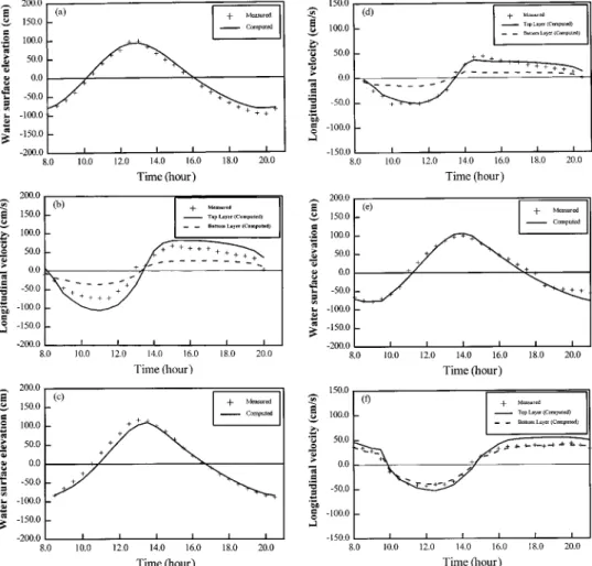
three 13-h time series of surface elevation and velocity at three stations each. No salinity data are available. Measurements were made at 30-min intervals over a full tidal cycle. Because of the shortage of field data for time series water surface elevations at the river mouth, a detailed calibration and verification such as that for the 1994 and 1995 conditions 共Hsu et al. 1999a兲 was not possible. Thus the constants in the turbulence model obtained from the 1994 and 1995 calibration/verification were assumed valid. The same values of Manning’s friction coefficient obtained from the 1994 and 1995 calibration/verification were also adopted for model verification with data of March 21, 1977. The model was run for 15 days with the observed 13-h surface elevation at the river mouth repeated for each tidal cycle as the open boundary condition. The measured daily river discharges over the corre-sponding 15-day period were used for the upstream boundary conditions. Fig. 5 shows comparisons between model results and field observations. The overall agreement between the model re-sults and field data are satisfactory, considering the lack of proper boundary conditions. Table 1 presents the mean absolute ences and root-mean-square differences that measure the differ-ences between the computed and measured time series data. They are comparable with those of model calibration/verification re-sults using 1994 and 1995 data共Hsu et al. 1999a兲. Therefore it is concluded that the same set of calibrated coefficients are appli-cable to conditions prior to reservoir construction.
Fig. 5. Model reverification results: comparisons of measured and computed results on March 21, 1977:共a兲 Water surface elevation at Tu-Ti-Kung-Pi;共b兲 longitudinal velocity at Tu-Ti-Kung-Pi; 共c兲 water surface elevation at Taipei Bridge; 共d兲 longitudinal velocity at Taipei Bridge; 共e兲 water surface elevation at Ta-Chih Bridge; and共f兲 longitudinal velocity at Ta-Chih Bridge
Model Application and Discussion
The reverified model was used to perform a series of model simu-lations to investigate salinity distributions before reservoir con-struction and under present conditions, respectively. The earliest available bathymetric data were collected in 1969, a time between the construction of the Shihman and Feitsui Reservoirs. These data共also presented in Fig. 3兲 were used to represent the geomet-ric conditions prior to reservoir construction.
To simulate the salinity distributions pre- and post-reservoir construction, respectively, model simulations were conducted using nine constituent tides. They were extracted from a harmonic analysis using field data at the river mouth in 1995. The nine constituents were M2共12.42 h兲, S2共12 h兲, N2共12.9 h兲, K1共23.93 h兲, Sa共8,765.32 h兲, O1共25.82 h兲, K2共11.97 h兲, P1共24.07 h兲, and M4共6.21 h兲. Amplitudes and phases of the tidal constituents were specified to generate a time series of surface elevations as a downstream boundary condition for a 1-year 共705 tidal cycle兲 model simulation. A high tide salinity of 35 ppt at the river mouth was used for model simulation. This is the typical value observed when river flow is below the long-term mean. The river dis-charges at the tidal limits of the three major tributaries, Tahan Stream, Hsintien Stream, and Keelung River, were specified as upstream boundary conditions. Table 2 lists the river discharges at upstream boundaries with mean flow (Qm), Q50flow共where Q50 is the flow that is equaled or exceeded for 50% of the time兲, and Q75flow before and after reservoir construction.
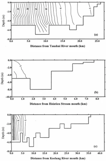
Figs. 6 and 7 present the predicted salinity distributions before and after reservoir construction, respectively, under Q50flow con-ditions. The computed salinities were averaged over 58 tidal cycles to smooth out the spring neap as well as the intratidal variations. The limits of salt intrusion after reservoir construction were farther up-river than that before reservoir construction in all three tributaries. This reflects the combined effects of the reduc-tion in river discharges and the deepening and widening of the river. The limits of salt intrusion, represented by 1 ppt isohaline, are located 22.5 and 25 km from the river mouth in the Tahan Stream before and after reservoir construction, respectively. The
surface salinity at the Keelung River mouth, where the Kuan-Du wetland is located, is of particular ecological significance. It con-trols the dominant vegetation types in the wetland. It increases from 12.5 to 15.8 ppt after reservoir construction. The patterns of salinity distributions under Qm and Q75flow conditions are simi-lar to those under Q50. They differ in the intrusion distance for specific isohaline. As the river flows decrease, the limits of salt intrusion move closer to the tidal limits and the difference be-tween pre- and post-reservoir construction reduces. However, the salinity differences in the lower and middle parts of the estuary remain substantial. Tables 3 and 4 present the summary results of
Fig. 6. Model prediction of salinity distributions before reservoir construction using Q50 flow condition: 共a兲 Tanshui River-Tahan
Stream;共b兲 Hsintien Stream; and 共c兲 Keelung River. 共The numbers on the contours refer to the salinity in parts per thousand.兲
Table 1.Mean Absolute Differences and Root-Mean-Square Differences between Computed and Measured Time Series Water Surface Elevation and Longitudinal Velocity for Model Reverification of March 21, 1977
Stations
Water surface elevation共cm兲 Longitudinal velocity共cm/s兲 共cross-sectional average兲 Mean absolute difference Root-mean-square difference Mean absolute difference Root-mean-square difference Tu-Ti-Kung-Pi 8.35 9.28 7.77 10.61 Taipei Bridge 7.71 10.51 11.47 13.95 Ta-Chih Bridge 7.75 9.95 4.80 6.51
Table 2. River Discharges at Upstream Boundaries before and after Reservoir Construction Conditions Upstream boundaries Qm 共m3/s兲 共mean flow兲 Q50 共m3/s兲 共medium flow兲 Q75 共m3/s兲 共low flow兲 Before reservoir construction Tahan Stream 69.82 29.65 18.10 Hsintien Stream 82.83 44.43 20.43 Keelung River 25.25 9.82 3.50 After reservoir Tahan Stream 41.04 12.75 4.03 Hsintien Stream 57.46 23.72 12.04 construction Keelung River 25.25 9.82 3.50
the salt intrusion limits in the Tahan Stream and the surface sa-linity in the river next to the Kuan-Du wetland under various river discharge conditions.
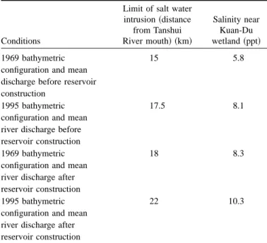
The above comparison of salinity distributions before and after the reservoir construction includes the combined effects of river discharge reduction and the enlargement of the river channel. To investigate each of the effects individually, two more model sce-nario runs were conducted. One run assumes the river geometry is unchanged while the mean river discharge is reduced after reser-voir construction. The other run assumes no reserreser-voir construc-tion while the river geometry has changed from 1969 to 1995 conditions. Table 5 summarizes the results of the scenario runs,
together with those pre- and post-reservoir conditions. It shows that the change in river geometry has almost the same effect as the reduction in river discharge.
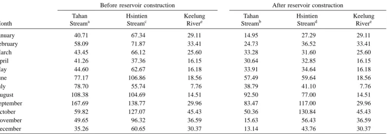
To examine the salinity change under the seasonally varying river discharge condition, another set of model simulations were conducted using average monthly flows before and after reservoir construction, respectively. Table 6 presents the average monthly flows at upstream boundaries of the three tributaries. It shows that the average monthly flows in the Tahan Stream and Hsintien Stream are significantly reduced after the reservoirs were con-structed. The only exception is for the month of October in the Hsintien Stream. The flows in the Keelung River were un-changed, since no reservoir was constructed there. A nine-constituent tide and a high tide salinity of 35 ppt at the river mouth were used to force the downstream boundary conditions.
Fig. 8 presents the simulation results of the time series salinity variation in the surface layer at the Keelung River mouth near the Kuan-Du wetland. The salinity fluctuates in response to the varia-tion of average monthly flows. However, the postreservoir condi-tion has the salinity higher than the prereservoir condicondi-tion at all times. The annual mean salinities before and after reservoir con-struction are 8.5 and 12.8 ppt, respectively. This suggests that the long-term salinity increases have the potential to favor the devel-opment of mangrove wetlands near the Keelung River mouth. In fact it has been suggested that salinity increase is the major culprit for the shift of vegetation types in the Kuan-Du wetland over the past 30 years 共Wester 1988兲. It has also been reported that the Fig. 7. Model prediction of salinity distributions after reservoir
con-struction using Q50flow condition:共a兲 Tanshui River-Tahan Stream;
共b兲 Hsintien Stream; and 共c兲 Keelung River. 共The numbers on the contours refer to the salinity in parts per thousand.兲
Table 3. Limit of Salt Water Intrusion in the Tahan Stream under Various River Discharge Conditions
Limit of salt water intrusion
共distance from Tanshui river
mouth兲 Before reservoir construction 共km兲 After reservoir construction 共km兲 Qm 15 22 Q50 22.5 25 Q75 23.5 25.5
Table 4. Salinity near the Kuan-Du Wetland under Various River Discharge Conditions
Salinity near Kuan-Du wetland共surface layer at the Keelung River mouth兲
Before reservoir construction 共ppt兲 After reservoir construction 共ppt兲 Qm 5.8 10.3 Q50 12.5 15.8 Q75 18.1 19.1
Table 5. Summary Results of Model Scenarios Using Mean Flow Condition
Conditions
Limit of salt water intrusion共distance from Tanshui River mouth兲 共km兲 Salinity near Kuan-Du wetland共ppt兲 1969 bathymetric
configuration and mean discharge before reservoir construction
15 5.8
1995 bathymetric configuration and mean river discharge before reservoir construction
17.5 8.1
1969 bathymetric configuration and mean river discharge after reservoir construction
18 8.3
1995 bathymetric configuration and mean river discharge after reservoir construction
salinity increase might contribute to the reduction of green algae in the lower part of the estuary共Wu 2000兲.
The development of mangrove wetlands gradually replaced the less salt-tolerant vegetation. The resultant change in vegetation density would alter the capacity of the shallow storage area for the vertical two-dimensional model, but its effect is considered minimal and not included in model simulations. On the other hand, it is expected that the growth of mangroves would have a significant impact on the flow field in the event of flood. Liu et al.
共2003兲 used a depth-averaged two-dimensional hydrodynamic
model to investigate the effects of mangrove trees on flow resis-tance. They found that the flow pattern and resistance distribution were quite different over the mangrove area during high flow events. Therefore the increasing development of mangrove wet-land would affect the resistance parameter used in a horizontal two-dimensional model.
Conclusions
A vertical 共laterally integrated兲 two-dimensional hydrodynamic and salt water intrusion numerical model was applied to the Tan-shui River estuarine system. The model had previously been cali-brated and verified with respect to the 1995 bathymertic configu-ration using observed time series water level, current, and salinity data of 1994 and 1995. The model was further reverified for the 1977 bathymetric configuration using limited data sets collected in 1977, the earliest intensive field survey conducted by the Tai-wan Water Resources Agency. The model was then used to simu-late the salinity distributions under different bathymetric configu-rations and for several scenarios of river flows before and after reservoir construction in the Tanshui River system.
The model simulations were conducted with three different constant river flow conditions, Qm, Q50, and Q75, at upstream boundaries of the three tributaries for the periods before and after reservoir construction. A nine-constituent tide and a high tide sa-linity of 35 ppt at the river mouth were used as the downstream boundary conditions. The results show that the limit of salt intru-sion moved farther up-river after the reservoirs were constructed. Substantial increases in salinity occurred throughout the estuary. Another set of model simulations was conducted using time vary-ing river flows at upstream boundaries. Each simulation was per-formed for 1 year with average monthly flows for the periods before and after reservoir construction, respectively. The results show that the surface salinity near Kuan-Du wetland increased at all times of the year and the annual mean salinities before and after reservoir construction were 8.5 and 12.8 ppt, respectively.
It has been speculated that the long-term increase in salinity is the driving force altering the aquatic ecosystem structure in the lower reach of the river system and Kuan-Du mangrove swamp. The most noticeable change is the expansion of mangrove areas and the disappearing of freshwater marshes. Though there was no concrete evidence for the cause of the salinity increase, land sub-sidence has been suggested. This case study concludes that the combined effects of the freshwater withdrawal at the reservoirs and the enlargement of the river channel could be the causes of Fig. 8. Computed time series salinity in the surface layer near
Kuan-Du wetland in the Keelung River
Table 6. Average Monthly Flows at the Upstream Boundaries of the Three Tributaries before and after Reservoir Construction
Month
Before reservoir construction After reservoir construction Tahan Streama Hsintien Streamc Keelung Rivere Tahan Streamb Hsintien Streamd Keelung Rivere January 40.71 67.34 29.11 14.95 27.29 29.11 February 58.09 71.87 33.41 24.73 36.52 33.41 March 43.45 66.12 25.60 33.28 31.60 25.60 April 41.26 37.36 16.15 30.64 32.85 16.15 May 44.60 62.67 16.18 33.91 34.64 16.18 June 77.17 106.86 18.56 57.49 59.64 18.56 July 78.70 55.74 7.76 38.79 41.10 7.76 August 108.38 104.69 14.51 92.50 77.00 14.51 September 167.69 138.77 29.96 83.47 117.00 29.96 October 59.82 127.07 45.43 50.36 130.84 45.43 November 49.65 96.32 36.59 15.63 56.43 36.59 December 35.26 60.65 30.37 13.14 43.76 30.37
aData collected from 1957 to 1964 before Shihman Reservoir was constructed. bData collected from 1965 to 1999 after Shihman Reservoir was constructed. cData collected from 1970 to 1986 before Feitsui Reservoir was constructed. dData collected from 1987 to 1999 after Feitsui Reservoir was constructed.
the change. The two alternations of the river system contribute to roughly the same degree of salinity increases.
Acknowledgments
This study is supported by National Science Council, Taiwan, under Grant No. 90-2211-E-002-086. The writers thank the Tai-wan Water Resources Agency for providing the prototype data. The writers also would like to express their appreciation to the three anonymous reviewers; through their comments this paper is substantially improved.
Notation
The following symbols are used in this paper:
Ax,Az ⫽ turbulent viscosity in x and z directions, respectively;
B ⫽ river width;
B ⫽ width at free surface including side storage area; g ⫽ gravitational acceleration;
H ⫽ total depth below mean sea level; h ⫽ depth;
Kx,Kz ⫽ turbulent dispersion coefficient and diffusivity in
x and z directions, respectively;
k ⫽ constant relating density to salinity (⫽7.5
⫻10⫺4/ppt); l ⫽ mixing length; p ⫽ pressure;
q ⫽ lateral inflow per unit river length; qp ⫽ lateral inflow per unit lateral area;
Ri ⫽ gradient Richardson number;
S0 ⫽ source and sink of salt due to exchange with side storage area;
s ⫽ laterally averaged salinity; t ⫽ time;
u ⫽ laterally averaged velocity in x direction; w ⫽ laterally averaged velocity in z direction;
x ⫽ distance seaward along river axis; Z ⫽ distance from the water surface;
z ⫽ distance upward in vertical direction;
␣, ⫽ constants;
兩u/z兩 ⫽ local value of vertical shear;
⫽ position of free surface above mean sea level; ⫽ water density;
m ⫽ stability function for momentum; and
s ⫽ stability function for mass.
References
Blumberg, A. F.共1977兲. ‘‘Numerical model of estuarine circulation.’’ J. Hydraul. Div., Am. Soc. Civ. Eng., 103共3兲, 295–310.
Blumberg, A. F.共1986兲. ‘‘Turbulent mixing processes in lakes, reservoirs, and impoundments.’’ Physics-based modeling of lakes, reservoir, and impoundments, W. G. Gray, ed., ASCE, New York, 79–104. Blumberg, A. F., Khan, L. A., and John, J. P. St. 共1999兲.
‘‘Three-dimensional hydrodynamic model of New York harbor region.’’ J. Hydraul. Eng., 125共8兲, 799–816.
Casulli, V., and Cheng, R. T. 共1992兲. ‘‘Semi-implicit finite difference methods for the three-dimensional shallow water flow.’’ Int. J. Numer. Methods Fluids, 15, 629– 648.
Dyer, K. R.共1973兲. Estuaries: A physical introduction, Wiley, New York. Festa, J. F., and Hansen, D. V.共1976兲. ‘‘A two-dimensional numerical model of estuarine circulation: the effects of altering depth and river
discharge.’’ Estuarine Coastal Mar. Sci., 4, 309–323.
Hall, R. W., and Chapman, R. S.共1985兲. ‘‘Two-dimensional QUICKEST; solution of the depth-average transport-dispersion equation.’’ Techni-cal Rep. EL-85-3, US Army Corps of Engineers, Vicksburg, Miss. Hsu, M. H., Kuo, A. Y., Kuo, J. T., and Liu, W. C.共1996兲. ‘‘Study of tidal
characteristics, estuarine circulation and salinity distribution in Tan-shui River system共I兲.’’ Technical Rep. No. 239, Hydrotech Research Institute, National Taiwan University, Taipei, Taiwan共in Chinese兲. Hsu, M. H., Kuo, A. Y., Kuo, J. T., and Liu, W. C.共1997兲. ‘‘Study of tidal
characteristics, estuarine circulation and salinity distribution in Tan-shui River system共II兲.’’ Technical Rep. No. 273, Hydrotech Research Institute, National Taiwan University, Taipei, Taiwan共in Chinese兲. Hsu, M. H., Kuo, A. Y., Kuo, J. T., and Liu, W. C.共1999a兲. ‘‘Procedure to
calibrate and verify numerical models of estuarine hydrodynamics.’’ J. Hydraul. Eng., 125共2兲, 166–182.
Hsu, M. H., Kuo, A. Y., Liu, W. C., and Kuo, J. T.共1999b兲. ‘‘Numerical simulation of circulation and salinity distribution in the Tanshui estu-ary.’’ Proc. Natl. Sci. Counc., Repub. China, Part A: Phys. Sci. Eng., 23共2兲, 259–273.
Johnson, B. H., Kim, K. W., Heath, R. E., Hsieh, B. B., and Butler, H. L. 共1993兲. ‘‘Validation of 3-D hydrodynamic model of Chesapeake Bay.’’ J. Hydraul. Eng., 119共1兲, 2–20.
Kjerfve, B.共1976兲. ‘‘The Santee-Cooper: A study of estuarine manipula-tions.’’ Estuarine processes, Vol. 1 M. Wiley, ed., Academic, Orlando, Fla., 44 –56.
Kjerfve, B., and Greer, J. E.共1978兲. ‘‘Hydrography of the Santee River during moderate discharge conditions.’’ Estuaries, 1, 111–119. Kuo, A. Y., and Liu, W. C.共2001兲. ‘‘Investigation of hydrodynamic
char-acteristics in the Tanshui River estuarine system.’’ 2001 Agricultural Engineering Annual Conference, Dept. of Agricultrual Engineering, National Taiwan Univ., Taipai, Taiwan, 1–13共in Chinese兲.
Lai, Y. G., Weber, L. J., and Patel, V. C.共2003兲. ‘‘Nonhydrostatic three-dimensional model for hydraulic flow simulation. I: Formulation and verification.’’ J. Hydraul. Eng., 129共3兲, 196–205.
Leonard, B. P., Vachtsevanos, G. J., and Abood, K. A.共1978兲. ‘‘Unsteady-state, two-dimensional salinity intrusion model for an estuary.’’ Ap-plied numerical modelling, C. Brebbia, ed., Pen Tech. Press, 113–123. Liu, W. C., Hsu, M. H., and Wang, C. F. 共2003兲. ‘‘Modeling of flow resistance in mangrove swamp at mouth of tidal Keelung River, Tai-wan.’’ J. Waterw., Port, Coastal, Ocean Eng., 129共2兲, 86–92. McAlice, B. J., and Jaeger, Jr., G. B.共1983兲. ‘‘Circulation changes in the
Sheepscot River estuary, Maine, following removal of a causeway.’’ Estuaries, 6, 190–199.
Park, K., and Kuo, A. Y.共1993兲. ‘‘A vertical two-dimensional model of estuarine hydrodynamics and water quality.’’ Special Report of Ap-plied Marine Science Sci. and Ocean Eng. No. 321, Virginia Institute of Marine Science, Gloucester Point, Va.
Park, K., and Kuo, A. Y.共1995兲. ‘‘A framework for coupling shoals and shallow embayments with main channels in numerical modeling of coastal plain estuaries.’’ Estuaries, 18共2兲, 341–350.
Pritchard, D. W.共1954兲. ‘‘A study of salt balance in a coastal plain estu-ary.’’ J. Mar. Res., 13共1兲, 133–144.
Pritchard, D. W.共1956兲. ‘‘The dynamic structure of a coastal plain estu-ary.’’ J. Mar. Res., 15共1兲, 33–42.
Roache, P. J.共1972兲. Computational fluid dynamics, Hermosa, Socorro, N.M.
Rossby, C. G., and Montgomery, R. B.共1935兲. ‘‘The layer of frictional influence in wind and ocean currents.’’ Physical oceanography and meteorology.
Talbot, J. W., and Talbot, G. A.共1974兲. ‘‘Diffusion in shallow seas and in English coastal and estuarine waters.’’ Rapp. P.-V. Reun.-Cons. Int. Explor. Mer, 167, 93–110.
Wang, I. Z.共1999兲. ‘‘An ecological study of estuarine wetlands-A case study of the changing vegetations of Kuan-Du mangrove swamp.’’ Masters thesis, National Taiwan University, Taipei, Taiwan共in Chi-nese兲.
Wang, J. D., Blumberg, A. F., Bulter, H. L., and Hamilton, P.共1990兲. ‘‘Transport prediction in partially stratified tidal water.’’ J. Hydraul. Eng., 116共3兲, 380–396.
Wang, L. L., Mysak, A., and Ingram, R. G.共1994兲. ‘‘A 3-D numerical simulation of Hudson Bay summer circulation.’’ J. Phys. Oceanogr., 24, 2496 –2514.
Wester, L.共1988兲. ‘‘Vegetation change in Kuan-Du marsh, Taiwan 1978– 1985.’’ Detailed planning of Kuan-Du National Park, Taipei City Government, Taipei, 415– 426.
Wu, J. T. 共2000兲. ‘‘Establishment of ecological monitoring system in Tanshui River estuary.’’ Report to Institute of Academic Sinica, Taipei, Taiwan共in Chinese兲.