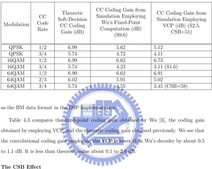
WiMAX 通道編碼技術與數位信號處理器實現之探討
144
0
0
全文
(2)
(3) WiMAX 通道編碼技術與 數位訊號處理器實現之探討 Study in WiMAX Channel Coding Techniques and Associated Digital Signal Processor Implementation. 研究生: 陳佳楓. Student: Jia-Fong Chen. 指導教授: 林大衛 博士. Advisor: Dr. David W. Lin. 國 立 交 通 大 學 電子工程學系. 電子研究所碩士班. 碩士論文. A Thesis Submitted to Department of Electronics Engineering & Institute of Electronics College of Electrical and Computer Engineering National Chiao Tung University in Partial Fulfillment of the Requirements for the Degree of Master of Science in Electronics Engineering June 2008 Hsinchu, Taiwan, Republic of China. 中華民國九十七年六月.
(4)
(5) WiMAX 通道編碼技術與 數位信號處理器實現之探討 研究生:陳佳楓. 指導教授:林大衛 博士. 國立交通大學 電子工程學系 電子研究所碩士班. 摘要 IEEE 802.16e 無線通訊標準中,於系統的傳送端訂定了前向誤差改正編碼的機 制,藉此減低通訊頻道中雜訊失真的影響。通道編碼是本論文的重點。 本篇論文前半部份重點在於,研究 IEEE 802.16e OFDMA 所訂定的迴旋編碼(咬 尾)系統並且實現在德州儀器公司所發展數位訊號處理器(DSP) TMS320C6416 上的維 特比解碼協處理器(VCP)並針對咬尾編碼的特性,中斷服務常式(ISR)以及增強型直接 記憶體存取(EDMA)進行研究。此外我們也利用 3L Diamond 的 EDMA 進行 VCP 在多 個 DSP 運算處理的應用。在論文中,我們利用 C 語言所模擬的迴旋碼在加成性白色 高斯通道下和利用 VCP 應用於迴旋碼進行效能及速度上的比較。在效能錯誤率上, 受限於實點數及 VCP 輸入位元數的硬體條件下,若以相同條件比較而言,兩者的效 能是接近的。而在速度方面,經過在 DSP 平台上最佳化我們的程式後,分別於 CCS 模 擬器和 3L 測量上,迴旋編碼的編碼器部份,可以到每秒 16,667K 和 3,764K 位元的處 理速度,而在 VCP 方面解碼器的部份可以達到每秒 7,897K 和 2,997K 位元的處理速 度,C 語言模擬方面則可以達到每秒 805K 和 632K 位元的處理速度。簡而說之,若 以解碼器觀點而言,VCP 提升了速度為 9.8 和 4.7 倍,分別針對 CCS 模擬器和 3L Diamond 測量而得到數據。 本論文後半部份重點,研究 IEEE 802.16e OFDMA 所訂定的渦輪迴旋碼(CTC)系 統並且實現在數位訊號處理器。闡明渦輪迴旋碼的雙二位元循環遞迴系統迴旋 (duo-binary CRSC)編碼與最大對數事後機率(max-log MAP)解碼演算法。我們利用 C 語言驗證系統演算法上的正確性,並在加成性白色高斯通道下模擬了各種調變。接著 在 TI C6416 DSP 平台實現,於 3L Diamond 測量上方面,編碼器部份可以到每秒 8,223 位元的處理速度,而解碼器的部份僅可以達到每秒 30K 位元的處理速度。之後我們對 於解碼器做了一些最佳化的改善,使解碼器的速度增進約 10 倍,進而可以達到每秒 300K 位元的處理速度。.
(6) Study in WiMAX Channel Coding Techniques and Associated Digital Signal Processor Implementation. Student: Jia-Fong Chen. Advisor: Dr. David W. Lin. Department of Electronics Engineering & Institute of Electronics National Chiao Tung University Abstract In the IEEE 802.16e wireless communication standard, a forward error correction (FEC) mechanism is presented at the transmitter side to reduce the noisy channel effect. The focus is on the channel coding. The focus of the fist part of this thesis is the research of the convolutional code (CC) with tail biting defined in IEEE 802.16e OFDMA standard and implement the project on Viterbi-decoder coprocessor (VCP) of the Texas Instruments (TI)’s TMS320C6416T digital signal processor (DSP) and also sturdy for tail-biting encoding property, interrupt service routine (ISR) and enhanced direct memory access (EDMA). Besides, we also employ the EDMA under 3L Diamond real-time operating system (RTOS) for the VCP applications of multi-DSP operation. We compare CC in AWGN channel on the C program to CC on the VCP applications for BER performance and processing rate. In BER performance, the simulation is limited to the hardware fixed-point and VCP branch metric input bit numbers; however, if we utilize the same condition to compare them, we can find their performance are close. In processing rate, after optimizing the programs on the DSP platform, encoder can achieve two data processing rates of 16,667 Kbps and 3,764 Kbps, the VCP decoder can achieve two processing rates of 7,897 Kbps and 2,997 Kbps and the C program decoder can achieve two processing rates of 805 Kbps and 632 Kbps, respectively on the C6416 CCS simulator and 3L Diamond. In short, we utilize the CCS and 3L to measure, finding decoding processing rate can be improve significantly about 9.8 and 4.7 times, respectively. The focus of second part is the research of the convolutional turbo code (CTC) defined in IEEE 802.16e OFDMA and implement on the C6416 DSP. We explain the duo-binary circular recursive systematic convolutional encoding (duo-binary CRSC) and the max-log MAP decoding algorithm. We employ the C program to insure the correctness of our.
(7) algorithm and simulate the CTC for different modulation in AWGN; then, we implement on TI C6416 DSP. The encoder can achieve a data processing rate of 8,223 Kbps and the decoder can achieve a processing rate of 30 Kbps on the 3L. Then we utilize some optimized techniques to improve the decoder's speed, which is approximately 10 times speeded up in decoding rate. Therefore, the decoder can achieve a further data processing rate of 300 Kbps..
(8)
(9) 誌謝 本篇論文的完成,誠摯地感謝我的指導老師林大衛博士,從踏入交通大學電 子所開始,多虧老師的循循善誘,不但給予我在課業、研究上的幫助,使我學到 了分析問題及解決問題的能力。同時老師樂觀的生活態度也影響了我,讓我更有 勇氣面對各種困難。在此,僅向老師及老師的家人致上最高的感謝之意。 另外要感謝的,是實驗室的洪崑健學長和吳俊榮學長。謝謝你們熱心有耐性 地幫我解決了許多通訊方面相關的疑問。也要感謝 3L Diamond Engineer Peter Robertson,謝謝你不嫌棄我的英文,透過不斷往來的英文書信,仍然很熱心很 積極的幫我解決一些 3L EDMA 的問題。另外還要感謝「數位信號處理平台在嵌 入式系統的應用」一書作者,交大電信所畢業的盧怡仁學長,學長已經畢業學校 很多年,因緣巧合和學長搭上了線,感謝您幫我釐清一些 DSP 問題的觀念。 感謝通訊電子與訊號處理實驗室(Commlab),提供了充足的軟硬體資源,讓 我在研究中不虞匱乏。感謝 94 級柏昇、順成兩位學長的指導,以及 95 級昀澤、 光中、婉清、奕安、威年、尚諭、衛川、紹唐等實驗室成員,平日和我一起唸書, 一起討論,也一起打混,讓我的研究生涯充滿歡樂又有所成長。期待大家畢業之 後都能有不錯的發展。 最後,要感謝的是我的家人,他們的支持讓我能夠心無旁騖的從事研究工作。 謝謝所有幫助過我、陪我走過這一段歲月的師長、同儕與家人。謝謝! 誌於 2008.6 故鄉風城 交大 佳楓.
(10)
(11) Contents. 1 Introduction. 1. 1.1. Scope of the Work . . . . . . . . . . . . . . . . . . . . . . . . . . . . . . . .. 1. 1.2. Organization of This Thesis . . . . . . . . . . . . . . . . . . . . . . . . . . .. 3. 2 Overview of CC and CTCs in IEEE 802.16e OFDMA 2.1. 2.2. 2.3. 4. Tail-Biting Convolutional Code Specifications [1] . . . . . . . . . . . . . . . .. 4. 2.1.1. Randomizer [1] . . . . . . . . . . . . . . . . . . . . . . . . . . . . . .. 5. 2.1.2. Convolutional Encoder [1] . . . . . . . . . . . . . . . . . . . . . . . .. 7. 2.1.3. Interleaver [1] . . . . . . . . . . . . . . . . . . . . . . . . . . . . . . .. 10. 2.1.4. Modulation [1] . . . . . . . . . . . . . . . . . . . . . . . . . . . . . .. 11. Decoding of CC . . . . . . . . . . . . . . . . . . . . . . . . . . . . . . . . . .. 11. 2.2.1. Demodulation for Bit-Interleaved Coded Modulation [9] . . . . . . . .. 12. Convolutional Turbo Codes Specifications [1] . . . . . . . . . . . . . . . . . .. 16. 2.3.1. CTC Encoder in IEEE 802.16e OFDMA [1] . . . . . . . . . . . . . .. 17. 2.3.2. CTC Interleaver [1] . . . . . . . . . . . . . . . . . . . . . . . . . . . .. 20. 2.3.3. CTC Tail-Biting [1], [10] . . . . . . . . . . . . . . . . . . . . . . . . .. 20. i.
(12) 2.3.4. 2.4. Subpacket Generation (Channel Interleaver or Interleaver and Puncturing) [1] . . . . . . . . . . . . . . . . . . . . . . . . . . . . . . . . .. 23. Decoding of CTC . . . . . . . . . . . . . . . . . . . . . . . . . . . . . . . . .. 29. 2.4.1. The Turbo Decoding Algorithm [11] . . . . . . . . . . . . . . . . . . .. 29. 2.4.2. Decoding Rule for CRSC Codes with Non-binary Trellis [14] . . . . .. 31. 2.4.3. Simplified Max-Log-MAP Algorithm for Double-Binary CTC [14] . .. 33. 3 DSP Implementation Environment. 37. 3.1. The DSP Baseboard . . . . . . . . . . . . . . . . . . . . . . . . . . . . . . .. 37. 3.2. The Viterbi-Decoder Coprocessor (VCP) [19] . . . . . . . . . . . . . . . . . .. 38. 3.2.1. Overview of VCP [19], [21], [22] . . . . . . . . . . . . . . . . . . . . .. 38. 3.2.2. VCP Inputs (Brach Metrics and VCP Input Configuration) [19], [22]. 43. 3.2.3. VCP Output (Decisions) [19]. . . . . . . . . . . . . . . . . . . . . . .. 46. 3.2.4. Sliding Windows Processing [19] . . . . . . . . . . . . . . . . . . . . .. 48. VCP Programming [19], [21] . . . . . . . . . . . . . . . . . . . . . . . . . . .. 49. 3.3. 3.3.1. 3.4. Prepare Input Configuration, Initialize Input Buffers, and Allocate Output Buffers [21] . . . . . . . . . . . . . . . . . . . . . . . . . . . .. 51. 3.3.2. EDMA Resource [19] . . . . . . . . . . . . . . . . . . . . . . . . . . .. 52. 3.3.3. VCP Procedure [21]. . . . . . . . . . . . . . . . . . . . . . . . . . . .. 52. EDMA under the Code Composer Studio (CCS) [23] . . . . . . . . . . . . .. 54. 3.4.1. EDMA Control Registers [23] . . . . . . . . . . . . . . . . . . . . . .. 55. 3.4.2. Parameter RAM (PaRAM) [23] . . . . . . . . . . . . . . . . . . . . .. 58. ii.
(13) 3.5. 3.4.3. EDMA Transfer Parameter Entry [23]. . . . . . . . . . . . . . . . . .. 60. 3.4.4. Initiating an EDMA Transfer [23] . . . . . . . . . . . . . . . . . . . .. 60. 3.4.5. Linking EDMA Transfers [23] . . . . . . . . . . . . . . . . . . . . . .. 61. 3.4.6. EDMA Interrupt Generation [23], [24]. . . . . . . . . . . . . . . . . .. 62. EDMA under the 3L Diamond Real-Time Operating System . . . . . . . . .. 64. 3.5.1. Introduction to 3L Diamond . . . . . . . . . . . . . . . . . . . . . . .. 64. 3.5.2. SC6xEDMA [26] . . . . . . . . . . . . . . . . . . . . . . . . . . . . .. 64. 3.5.3. EDMA Channel Availability [26] . . . . . . . . . . . . . . . . . . . .. 67. 3.5.4. SC6xEDMAChannel Functions [26] . . . . . . . . . . . . . . . . . . .. 67. 4 DSP Implementation of Convolutional Encoder and Decoder 4.1. 70. VCP Parameter Setting . . . . . . . . . . . . . . . . . . . . . . . . . . . . .. 70. 4.1.1. Generator Polynomials . . . . . . . . . . . . . . . . . . . . . . . . . .. 71. 4.1.2. EDMA Setting . . . . . . . . . . . . . . . . . . . . . . . . . . . . . .. 71. 4.1.3. Tail-Biting . . . . . . . . . . . . . . . . . . . . . . . . . . . . . . . . .. 72. 4.2. Coding Gain Analysis [3] . . . . . . . . . . . . . . . . . . . . . . . . . . . . .. 73. 4.3. Comparison of Performance in AWGN of VCP and Wu’s Viterbi Decoder . .. 75. 4.4. VCP Operation Under 3L Diamond . . . . . . . . . . . . . . . . . . . . . . .. 84. 5 Simulation and DSP Implementation of CTC Encoder and Decoder. 89. 5.1. Performance in AWGN Channel with Floating-Point Processing . . . . . . .. 89. 5.2. Performance in AWGN Channel with Fixed-Point Processing . . . . . . . . .. 91. iii.
(14) 5.3. 5.2.1. Speed Performance of the DSP Code . . . . . . . . . . . . . . . . . .. 5.2.2. Improving CTC Decoding Speed. 97. . . . . . . . . . . . . . . . . . . . . 101. Comparison of Speed of Current Codes . . . . . . . . . . . . . . . . . . . . . 113 5.3.1. The Views of Block Decoder for Processing Rate . . . . . . . . . . . . 113. 5.3.2. Comparison of Tail-Biting CC and CTC for Adders and Multipliers . 114. 5.3.3. Comparison of Decoder Speed for Tail-Biting CC, CTC, and LDPC . 116. 6 Conclusion and Future Work. 118. Bibliography. 120. iv.
(15) List of Figures 2.1. Structure of convolutional coding in transmitter (top path) and decoding in receiver (bottom path). . . . . . . . . . . . . . . . . . . . . . . . . . . . . . .. 5. 2.2. PRBS for data randomization (from [1]).. . . . . . . . . . . . . . . . . . . .. 7. 2.3. Convolutional encoder of rate 1/2 (from [1]). . . . . . . . . . . . . . . . . . .. 8. 2.4. The second permutation of interleaver. . . . . . . . . . . . . . . . . . . . . .. 11. 2.5. QPSK, 16-QAM, and 64-QAM constellations (from [1]).. . . . . . . . . . . .. 12. 2.6. Metric partitions of the 16-QAM constellation (from [9]). . . . . . . . . . . .. 15. 2.7. CTCs coding block diagram (from [1]). . . . . . . . . . . . . . . . . . . . . .. 16. 2.8. CTC encoder (modified from [1]). . . . . . . . . . . . . . . . . . . . . . . . .. 18. 2.9. CTC rate 1/3 encoder flow chart. . . . . . . . . . . . . . . . . . . . . . . . .. 19. 2.10 CTC encoding slot concatenation for different rate (modified from [1]). . . .. 20. 2.11 CTC channel coding per modulation (modified from [1]). . . . . . . . . . . .. 21. 2.12 CTC interleaver in two steps (modified from [1]). . . . . . . . . . . . . . . .. 22. 2.13 Block diagram of CTC channel interleaving scheme (from [1]). . . . . . . . .. 26. 2.14 Block diagram of a turbo decoder (from [11]). . . . . . . . . . . . . . . . . .. 29. v.
(16) 2.15 CTC trellis structure of duo-binary convolutional code with feedback encoder (from [14]). . . . . . . . . . . . . . . . . . . . . . . . . . . . . . . . . . . . .. 31. 3.1. Sundance’s SMT395 module (from [18]). . . . . . . . . . . . . . . . . . . . .. 38. 3.2. VCP block diagram (modified from [19]). . . . . . . . . . . . . . . . . . . . .. 39. 3.3. DSP chip architecture (from [20]). . . . . . . . . . . . . . . . . . . . . . . . .. 40. 3.4. DSP chip die (from [20]). . . . . . . . . . . . . . . . . . . . . . . . . . . . . .. 40. 3.5. Convolutional encoder example, where K = 3, R = 1/3, G0 = (100)8 , G1 = (101)8 , G2 = (111)8 (from [19]). . . . . . . . . . . . . . . . . . . . . . . . . .. 42. 3.6. Convolutional code trellis example (from [19]). . . . . . . . . . . . . . . . . .. 43. 3.7. Example of survivor path and associated decoded sequence (from [21]). . . .. 44. 3.8. VCP input FIFO (modified from [19]). . . . . . . . . . . . . . . . . . . . . .. 45. 3.9. VCP registers (modified from [19]). . . . . . . . . . . . . . . . . . . . . . . .. 46. 3.10 VCP configuration structure (modified from [22]). . . . . . . . . . . . . . . .. 47. 3.11 VCP output FIFO (modified from [19]). . . . . . . . . . . . . . . . . . . . .. 47. 3.12 VCP tailed traceback mode (from [19]). . . . . . . . . . . . . . . . . . . . . .. 49. 3.13 VCP frame, reliability, and convergence length limitations(modified from [19]). 50 3.14 VCP EDMA parameters structure (from [19]). . . . . . . . . . . . . . . . . .. 53. 3.15 EDMA control (from [23]). . . . . . . . . . . . . . . . . . . . . . . . . . . . .. 55. 3.16 EDMA parameter RAM contents (modified from [23]). . . . . . . . . . . . .. 59. 3.17 EDMA channel parameters (from [23]). . . . . . . . . . . . . . . . . . . . . .. 60. 3.18 Example of linked EDMA transfers (from [23]). . . . . . . . . . . . . . . . .. 62. vi.
(17) 4.1 CC encoding and decoding with VCP.. . . . . . . . . . . . . . . . . . . . . .. 71. 4.2. VCP parameter setting (modified from [21]). . . . . . . . . . . . . . . . . . .. 72. 4.3. Tail-biting CC decoding employing (modified from [3]). . . . . . . . . . . . .. 73. 4.4. VCP decoding performance in AWGN with different BM truncation precisions (1/3). . . . . . . . . . . . . . . . . . . . . . . . . . . . . . . . . . . . . . . .. 4.5. VCP decoding performance in AWGN with different BM truncation precisions (2/3). . . . . . . . . . . . . . . . . . . . . . . . . . . . . . . . . . . . . . . .. 4.6. 81. Effect of CSB values in VCP-based decoding in AWGN at different codingmodulation settings (2/3). . . . . . . . . . . . . . . . . . . . . . . . . . . . .. 4.9. 80. Effect of CSB values in VCP-based decoding in AWGN at different codingmodulation settings (1/3). . . . . . . . . . . . . . . . . . . . . . . . . . . . .. 4.8. 79. VCP decoding performance in AWGN with different BM truncation precisions (3/3). . . . . . . . . . . . . . . . . . . . . . . . . . . . . . . . . . . . . . . .. 4.7. 78. 82. Effect of CSB values in VCP-based decoding in AWGN at different codingmodulation settings (3/3). . . . . . . . . . . . . . . . . . . . . . . . . . . . .. 83. 4.10 How VCP operates under 3L Diamond and TI CCS. . . . . . . . . . . . . . .. 84. 5.1. Performance of CTC at different iteration counts under different modulations. 90. 5.2. CTC decoding performance with different modulations employing floatingpoint computation at 4 iterations. . . . . . . . . . . . . . . . . . . . . . . . .. 91. 5.3. CTC fixed-point truncation parameters. . . . . . . . . . . . . . . . . . . . .. 93. 5.4. CTC fixed-point truncation parameters flow chart. . . . . . . . . . . . . . . .. 93. 5.5. CTC at different bit numbers with different modulations. . . . . . . . . . . .. 94. vii.
(18) 5.6 Performance with scaling of various quantities in CTC decoding to avoid overflow at high SNR. . . . . . . . . . . . . . . . . . . . . . . . . . . . . . . . . . 5.7. 95. BER performance of CTC decoding with fixed-point computation vs. floatingpoint computation. . . . . . . . . . . . . . . . . . . . . . . . . . . . . . . . .. 96. 5.8. Function Gamma() (1/3). . . . . . . . . . . . . . . . . . . . . . . . . . . . . 103. 5.9. Function Gamma() (2/3). . . . . . . . . . . . . . . . . . . . . . . . . . . . . 104. 5.10 Function Gamma() (3/3). . . . . . . . . . . . . . . . . . . . . . . . . . . . . 105 5.11 The assembly code of Gamma() function (1/6). . . . . . . . . . . . . . . . . 106 5.12 The assembly code of Gamma() function (2/6). . . . . . . . . . . . . . . . . 107 5.13 The assembly code of Gamma() function (3/6). . . . . . . . . . . . . . . . . 108 5.14 The assembly code of Gamma() function (4/6). . . . . . . . . . . . . . . . . 109 5.15 The assembly code of Gamma() function (5/6). . . . . . . . . . . . . . . . . 110 5.16 The assembly code of Gamma() function (6/6). . . . . . . . . . . . . . . . . 111. viii.
(19) List of Tables 2.1. Mandatory Channel Coding Schemes for Each Modulation Method . . . . .. 6. 2.2. The Convolutional Code with Puncturing Configuration. . . . . . . . . . . .. 8. 2.3. Bit Interleaved Block Sizes and Modulos . . . . . . . . . . . . . . . . . . . .. 10. 2.4. Bit Metric for Method-ML and Method-LLR. . . . . . . . . . . . . . . . . .. 14. 2.5. Circulation State Look-Up Table (SC1 and SC2 ) . . . . . . . . . . . . . . . .. 23. 2.6. Parameters for the Subblock Interleavers . . . . . . . . . . . . . . . . . . . .. 26. 3.1. Branch Metrics for Rate-1/2 Code. . . . . . . . . . . . . . . . . . . . . . . .. 44. 3.2. VCP Required EDMA Links Per User Channel . . . . . . . . . . . . . . . . .. 50. 3.3. EDMA Control Registers (Modified from [23]) . . . . . . . . . . . . . . . . .. 56. 4.1. Coding Gain Upper Bounds in AWGN at BER = 10−6 . . . . . . . . . . . .. 75. 4.2. Approximate Coding Gains Based on Analysis of Minimum Codeword Distance. . . . . . . . . . . . . . . . . . . . . . . . . . . . . . . . . . . . . . . .. 76. 4.3. Comparison of Soft-Decision Decoding Performance, in AWGN at BER = 10−6 77. 4.4. Speed of Overall Decoder from 3L-Measured Execution Time . . . . . . . . .. 85. 4.5. CCS Profile of CC Coding and Decoding with VCP (Cycles) . . . . . . . . .. 86. ix.
(20) 4.6 3L-Measured Execution Time of CC Coding and Decoding with VCP (ms) . 4.7. Information Data Processing Rate Calculated from CCS Profile of CC with VCP . . . . . . . . . . . . . . . . . . . . . . . . . . . . . . . . . . . . . . . .. 4.8. . . . . . . . . . . . . . . . . . . . . . . . . . . . . . . . . . . . . . .. 92. Coding Gain Performance of Rate-1/3 CTC in AWGN at BER = 10−5 with Floating-Point and Fixed-Point Computation. 5.3. 88. Comparison of Coding Gains of CTC and Tail-biting CC in AWGN at BER = 10−6. 5.2. 87. Information Data Processing Rate Calculated from 3L-Measure Execution Time of CC with VCP . . . . . . . . . . . . . . . . . . . . . . . . . . . . . .. 5.1. 87. . . . . . . . . . . . . . . . . .. 96. CTC Rate-1/3 Encoder Execution Times Measured under 3L and the Corresponding Data Rate with 480-Bit Information Data Blocks . . . . . . . . . .. 98. 5.4. Profile of CT C Encoder with QPSK Modulation for One Data Block . . . .. 98. 5.5. CTC Rate-1/3 Decoder Executive Times for 480 Information Bits Measured under 3L . . . . . . . . . . . . . . . . . . . . . . . . . . . . . . . . . . . . . .. 5.6. 99. Corresponding Processing Rates of CTC Rate-1/3 Decoder Based on 3LMeasured Execution Times for One Information Data Block of 480 Bits . . . 100. 5.7. Profile of CT C Decoder with QPSK Modulation for One Data Block in One Iteration . . . . . . . . . . . . . . . . . . . . . . . . . . . . . . . . . . . . . . 100. 5.8. Profile of Duo Binnary CRSC Decoder . . . . . . . . . . . . . . . . . . . . 100. 5.9. Rate-1/3 CTC Processing Rate with 4 iterations in Decoding . . . . . . . . . 101. 5.10 Profile of Improved Duo Binnary CRSC Decoder . . . . . . . . . . . . . . 102. x.
(21) 5.11 Speed up in Decoding of One Data Block with QPSK Modulation for One Iteration . . . . . . . . . . . . . . . . . . . . . . . . . . . . . . . . . . . . . . 105 5.12 Improved CTC Decoding Speed Base on 3L-Measured Execution Times for One Information Data Block of 480 Bits . . . . . . . . . . . . . . . . . . . . 112 5.13 CTC Code Sizes . . . . . . . . . . . . . . . . . . . . . . . . . . . . . . . . . . 112 5.14 CC and CTC for Adder and Multiplier (Numbers) . . . . . . . . . . . . . . . 115 5.15 Information Data Processing Rate Calculated from CCS for One Information Data Block of 480 Bits . . . . . . . . . . . . . . . . . . . . . . . . . . . . . . 116 5.16 Comparison of Decoder Speed for Tail-Biting CC, CTC, and LDPC Calculated from CCS . . . . . . . . . . . . . . . . . . . . . . . . . . . . . . . . . . . . . 116. xi.
(22) Chapter 1 Introduction 1.1. Scope of the Work. Digital wireless transmission is a trend in the next generation of consumer electronics. Due to this demand high data transmission rate and mobility are needed. The OFDM modulation technique for wireless communication has been a main stream in recent years. IEEE has completed several standards, including the IEEE 802.11 series for LANs (local area networks) and IEEE 802.16 series for MANs (metropolitan area networks), based on OFDM technique. Our study is based on the IEEE 802.16e standard, which specifies the air interface of mobile broadband wireless multiple access systems providing multiple access. In wireless communication, the transmitted signals are easily interfered and distorted by variance things sources such as the crowd traffic, bad weather, the obstacle of buildings, etc. Digital wireless transmission with multimedia contents such as audio and video is a trend. These services often exhibit high data rates and require high quality reproduction. To improve the robustness of the wireless communication against the noisy channel condition, the FEC (forward-error-correcting coding) mechanism is a must in almost every commercial communication standard, including the IEEE 802.16e. CC (convolutional code) with tail-biting and CTCs (convolutional turbo codes) comprise 1.
(23) the mandatory channel coding schemes in Mobile WiMAX. A growing number of research studies are now available to shed some light on the convolution code and turbo code. A number of studies have been conducted using viterbi algorithm as the convolution decoding and BCJR algorithm as the turbo decoding. There have been numerous studies in the literature dealing with different decoding algorithms. However we need to reduce the complexity for actual DSP implementation. In convolution code, the TI C6416 is equipped with a Viterbi-decoder coprocessor (VCP) [19]. Using this coprocessor can be helpful in raising the decoding speed. Furthermore, we also consider runnig the VCP under 3L Diamond RTOS for more digital signal processors (DSPs) applications. In addition, We also discuss the CTC in IEEE 802.16e for OFDMA. It uses a double binary circular recursive systematic convolutional (CRSC) code, which makes CTC efficient for coding of data cells in blocks. Note that “circular” can be equated with tail-biting, which means the initial state of the encoding start frame to be the same as the end state of the encoding end frame. In this thesis, my work can be summarized as following: • Study IEEE 802.16e specifications. • Study tail-biting CC. – Study TI Viterbi-decoder coprocessor (VCP) and 3L Diamond EDMA. – Design tail-biting CC with VCP. • Study CTCs. – Design rate-1/3 CTC floating-point and fixed-point versions. – Compare the performance and complexity. – Use optimization methods to implement CTC on DSP. 2.
(24) 1.2. Organization of This Thesis. This thesis is organized as follows. • Chapter 2 introduces CC with tail-biting and the CTC (convolution turbo code) of IEEE 802.16e specifications. • Chapter 3 describes the DSP implementation environment, which is composed of the VCP, TI EDMA, and 3L EDMA. • Chapter 4 discusses simulation and the DSP implementation of the convolutional decode with VCP. • Chapter 5 discusses simulation and the DSP implementation of the CTC encoder and decoder. • Chapter 6 contains the conclusion and points out some future work.. 3.
(25) Chapter 2 Overview of CC and CTCs in IEEE 802.16e OFDMA Convolutional code with tail-biting and convolutional turbo codes comprise the mandatory channel coding schemes in Mobile WiMAX. In this chapter, we introduce their specifications in IEEE 802.16e and their decoding methods.. 2.1. Tail-Biting Convolutional Code Specifications [1]. The contents of this section have been taken to a large extent from [2], [3]. The mandatory channel coding scheme used in IEEE 802.16e OFDMA is as shown in Fig. 2.1. The input data stream is processed by the randomizer to clean up the bit correlation, and then each data block is encoded by the convolutional encoder with tail-biting, which means the encoder starts in the same state as it ends up after encoding. The block-by-block coding makes the convolutional code effectively a block code. However, we do not implement the repetition block, which can be used to further increase signal margin over the modulation and FEC mechanisms, for the channel coding procedures in IEEE 802.16e. As the repetition block can be applied only to QPSK modulation, we bypass it in the present study. The reader interested in the repetition block can refer to 4.
(26) Figure 2.1: Structure of convolutional coding in transmitter (top path) and decoding in receiver (bottom path). relevant material in [1]. We note again that our study concerns convolutional code with tail-biting, because an optional channel coding scheme of IEEE 802.16e is convolutional code with zero-tailing, which means the encoder is forced to return to the all-zero state after encoding. The two can be confused easily. Between the convolutional encoder and the modulator is a bit interleaver, which protects the convolutional code from severe impact of burst errors and increases overall coding performance. This approach has been termed “bit-interleaved coded modulation (BICM)” in the literature [4]. To make the system more flexibly adaptable to the channel condition, 19 coding-modulation schemes are defined in IEEE 802.16e, as shown in Table 2.1. The different coding rates are made by puncturing of the native convolutional code. The puncturing mechanism in convolutional coding can provide variable code rates through one convolutional encoder.. 2.1.1. Randomizer [1]. The randomizer is a pseudo random binary sequence (PRBS) generator defined by the polynomial 1 + X 14 + X 15 , as depicted in Fig. 2.2. Data randomization is performed on all data transmitted on the downlike (DL) and uplink (UL), expect the frame control header (FCH). The randomization is initialized on each FEC block. 5.
(27) Table 2.1: Mandatory Channel Coding Schemes for Each Modulation Method Modulation. Uncoded Block Size (bytes). Overall Code Rate. Coded Block Size (bytes). Number of Used Sub-channels. QPSK QPSK QPSK QPSK QPSK QPSK QPSK QPSK QPSK QPSK 16QAM 16QAM 16QAM 16QAM 16QAM 64QAM 64QAM 64QAM 64QAM. 6 12 18 24 30 36 9 18 27 36 12 24 36 18 36 18 36 24 27. 1/2 1/2 1/2 1/2 1/2 1/2 3/4 3/4 3/4 3/4 1/2 1/2 1/2 3/4 3/4 1/2 1/2 2/3 3/4. 12 24 36 48 60 72 12 24 36 48 24 48 72 24 48 36 72 36 36. 1 2 3 4 5 6 1 2 3 4 1 2 3 1 2 1 2 1 1. 6.
(28) Figure 2.2: PRBS for data randomization (from [1]).. If the amount of data to transmit does not fit exactly the amount of data allocated, padding of 0xFF (“1” only) shall be added to the end of the transmission block, up to the amount of data allocated. Here, the amount of data allocated means the amount of data that corresponds to the amount of slots bNs /Rc, where Ns is the number of the slots allocated for the data burst and R is the repetition factor used. Each data byte to be transmitted shall enter sequentially into randomizer, msb first, to make the “0” and “1” bits in the input data streams well-distributed and hence improve the coding performance. The randomization is applied only to information bits. Preambles are not randomized. In both UL and DL, the randomizer is initialized with the vector (LSB) 0 1 1 0 1 1 1 0 0 0 1 0 1 0 1 (MSB). As we do not implement the HARQ mechanism, we bypass it in the present study. Note that the randomizer can be initialized with different vector for HARQ required, which can refer to [1] in detail.. 2.1.2. Convolutional Encoder [1]. Each block is encoded by a binary convolutional encoder, which has native rate 1/2 and constraint length 7. The generator polynomials for the two output bits are 171OCT and 133OCT , respectively, as depicted in Fig. 2.3. 7.
(29) Figure 2.3: Convolutional encoder of rate 1/2 (from [1]). Table 2.2: The Convolutional Code with Puncturing Configuration. Rate Dfree X Y XY. 1/2 10 1 1 X1 Y1. Code Rates 2/3 6 10 11 X1 Y1 Y2. 3/4 5 101 110 X1 Y1 Y2 X3. The coded bits may be punctured to allow different rates, which is known as ratecompatible punctured convolutional coding (RCPC). Furthermore, tail-biting is performed, by initializing the encoder’s memory with the last 6 data bits of the block. Punctured Convolutional Code Puncturing patterns and serialization order of the convolutional code in IEEE 802.16e are as defined in Table 2.2. In this table, “1” means a transmitted bit and “0” a removed bit, whereas X and Y are in reference to Fig. 2.3. Note that the Dfree after puncturing is lower than that of the native convolutional code at rate 1/2, which is equal to 10 [8, Chapter 8].. 8.
(30) Tail-Biting The CC in IEEE 802.16e is terminated in a block; it therefore becomes a block code. In general, there are three methods to achieve code termination [5]. For ease of understanding, we describe these methods in terms of a binary (n, k, m) CC (of rate k/n and register length m) for an information sequence length of L bits. • Direct truncation. The codeword is produced by inputting into the encoder (initialized with all zeros) L information bits, so the codeword length is nL/k. However, this code has the disadvantage that there is lower error protection ability afforded to the last information bits. • Zero tail. The codeword is produced by inputting into the encoder (initialized with all zeros) L information bits followed by m zeros (tail bits), so the codeword length is n(L + m)/k. This code has the disadvantage of rate loss of m/(L + m) since the effective rate is (k/n)(L/(L + m)) = (k/n)(1 − m/(L + m)). • Tail biting. We first initialize the encoder with the last m information bits, and then inputting into the encoder L information bits to produce codeword whose length is nL/k. This code has the disadvantage of complex Viterbi decoding since the starting and ending states of the trellis are unknown. IEEE 802.16e uses the tail-biting approach, which has better performance compared with direct-truncation CC and does not lose rate compared with zero-tail CC. Nevertheless, we pay the price of a complex decoder. The optimal decoder of tail-biting convolutional code, as suggested in [5], is to run M parallel Viterbi decoders, where M = 2m is the number of states in the trellis. Each Viterbi decoder postulates a different starting and ending state. The Viterbi decoder that produces the globally best metric gives the maximum likelihood 9.
(31) Table 2.3: Bit Interleaved Block Sizes and Modulos. Modulation. Coded Bits per Subcarrier (Ncpc ). Modulo used (d). QPSK 16QAM 64QAM. 2 4 6. 16 16 16. estimate of the transmitted bits. The obvious disadvantage of this method is the M times complexity compared to decoding for the code with zero tail bits. Therefore, we consider a suboptimal decoder which can reduce the complexity to less than 2 times the normal Viterbi algorithm. This decoder combines the algorithms proposed in [6] and [7] and will be introduced later.. 2.1.3. Interleaver [1]. The encoded data bits are interleaved by a block interleaver with a block size corresponding to the number of coded bits per the specified allocation, Ncbps (see Table 2.3). The interleaver is defined by a two-step permutation. The first ensures that adjacent coded bits are mapped onto non-adjacent carriers. The second insures that adjacent coded bits are mapped alternately onto less or more significant bits of the constellation, thus avoiding long runs of lowly reliable bits. Let s = Ncpc /2, k be the index of the coded bit before the first permutation, m the index after the first and before the second permutation and j the index after the second permutation, just prior to modulation mapping. The first permutation is defined by m=(. Ncbps k ) · kmod(d) + f loor( ), d d. 10. k = 0, 1, · · · , Ncbps − 1,. (2.1).
(32) Figure 2.4: The second permutation of interleaver. and the second permutation is defined by j = s · f loor(. m d·m ) + (m + Ncbps − f loor( ))mod(s), s Ncbps. m = 0, 1, · · · , Ncbps − 1.. (2.2). The first permutation is a block interleaving. And in Fig. 2.4, we show the second permutation after the block interleaving.. 2.1.4. Modulation [1]. After bit interleaving, the data bits are entered serially to the constellation mapper. Graymapped QPSK and 16-QAM are supported, whereas the support of 64-QAM is optional. The constellations as shown in Fig. 2.5 shall be normalized by multiplying the constellation points with the indicated factor c to achieve equal average power. The constellation-mapped data shall be subsequently modulated onto the allocated data carriers.. 2.2. Decoding of CC. In this section, we introduce the decoding method for CC. As there is a bit interleaver between the convolutional encoder and the modulator in the transmitter, the decoder should be based on the super-trellis combining the convolutional code, the interleaver, and the QAM 11.
(33) Figure 2.5: QPSK, 16-QAM, and 64-QAM constellations (from [1]).. modulator. So we mainly introduce the demodulation for bit-interleaved modulation in the section. For decoding of CC with tail-biting, we discuss it in chapter 3 along with the VCP and discuss how to do tail-biting with the VCP in chapter 4.. 2.2.1. Demodulation for Bit-Interleaved Coded Modulation [9]. Let a[i] = aI [i] + jaQ [i] denote the QAM symbol transmitted in the ith sub-carrier of OFDMA symbol and {bI,1 , · · · , bI,k , · · · , bI,t , bQ,1 , · · · , bQ,k , · · · , bQ,t } be the corresponding bit sequence. Assuming that the ISI (inter–OFDMA symbol interference) and ICI (inter– channel interference) are completely eliminated, we can write the received signal of the sub-carrier as r[i] = Gch [i] · a[i] + w[i],. (2.3). where Gch [i] is the complex channel frequency response at the ith sub-carrier and w[i] is the complex additive white Gaussian noise (AWGN) with variance σ 2 = N0 . If the channel. 12.
(34) estimate is error free, the output of the one-tap equalizer is given by y[i] = a[i] + w[i]/Gch [i] = a[i] + w0 [i],. (2.4). where w0 [i] is still complex AWGN noise with variance σ 02 (i) = σ 2 /|Gch [i]|2 . According to the MAPSE (maximum a posterior sequence estimation) criterion, the following maximization should be performed to estimate the encoded bit sequence b: ˆ = arg max P [b|r], b. (2.5). b. where r is the received sequence of QAM signals. Assume that the transmitted symbols are equally distributed. Then the MAPSE criterion can be replaced by the ML (maximum likelihood) criterion as: ˆ = arg max P [r|b]. b. (2.6). b. We further assume that Gch [i] is known to the receiver and that the transmitted bits are independent and identically distributed (i.i.d.). For each in-phase or quadrature bit (i.e., bI,k or bQ,k ), two metrics can be derived corresponding to the two possible values 0 and 1, respectively. For bit bI,k , first the QAM (0). constellation is split into two partitions of complex symbols, namely SI,k comprising the (1). symbols with a “0” in position (I, k) and SI,k , which is complementary. Then the two metrics are obtained by m0c (bI,k ) =. X. log p(r[i]|a[i] = α) ≈ max log p(r[i]|a[i] = α), (c). c = 0, 1.. (2.7). α∈SI,k. (c). α∈SI,k. Since the conditional pdf of r[i] is complex Gaussian as p(r[i]|a[i] = α) = √. 1 1 |r[i] − Gch [i]α|2 } exp{− 2 σ2 2πσ. (2.8). and r[i] = Gch [i] · y[i], the metrics defined in (2.35) are equivalent to mc (bI,k ) = |Gch [i]|2 · min |y[i] − α|2 . (c). α∈SI,k. 13. (2.9).
(35) Table 2.4: Bit Metric for Method-ML and Method-LLR Bit metric (decided “0”) Bit metric (decided “1”). Method-ML m0 m1. Method-LLR − m1 ) + 1)]2 − m1 ) − 1)]2. [ 41 (m0 [ 41 (m0. Finally, these metrics are de-interleaved, i.e., each couple (m0 , m1 ) is assigned to the bit position in the decoded sequence according to the de-interleaver map, and fed to the Viterbi decoder which selects the binary sequence with the smallest cumulative sum of metrics. We name this method Method-ML in the following discussion. From the concept of log-likelihood ratio (LLR), a method named Method-LLR is proposed in [9] to reduce the complexity of Method-ML. It defines LLR(bI,k ) as LLR(bI,k ) ,. |Gch [i]|2 { min |y[i] − α|2 − min |y[i] − α|2 } (0) (1) 4 α∈SI,k α∈SI,k. , (m0 (bI,k ) − m1 (bI,k ))/4 , |Gch [i]|2 · DI,k .. (2.10). The quadrature part is similarly defined. The metrics sent to the Viterbi decoder in the two methods are defined in Table 2.4. Note that the difference between the bit metrics for the decided “0” and “1” is the same for the two methods, namely ±(m0 − m1 ). Thus the decoded bit sequence will be the same for the two methods. In Method-LLR, only (m0 − m1 )/4 is sent to the de-interleaver while in Method-ML, both m0 and m1 are sent. Besides, we can reduce (m0 − m1 )/4 = |Gch [i]|2 · DI,k to a simple form constituting of yI [i] itself because Gray coding is used in the constellation map of M -ary QAM modulation in IEEE 802.16e. (0). (1). Figure 2.6 shows the partitions of (SI,k , SI,k ) for the generic bit bI,k in the case of 16-QAM.. 14.
(36) Q. Q. x. x. I. I −3 (11). S I,11. −1(10). 1 (00). 3 (01). S I,10. BI,1. −3(11). −1(10). S I,21. S I,20. 1 (00). 3 (01). S I,21. BI,2. Figure 2.6: Metric partitions of the 16-QAM constellation (from [9]). As a consequence, 1 DI,k = { min |y[i] − α|2 − min |y[i] − α|2 } (0) (1) 4 α∈SI,k α∈SI,k can be simplified as follows. DI,1 DI,2. |yI (i)| ≤ 2 −yI [i], −2(yI [i] − 1), yI (i) > 2 = −2(yI [i] + 1), yI (i) < 2 = |yI [i]| − 2.. ∼ = −yI [i],. (2.11) (2.12). The same observation holds for QPSK and 64-QAM constellations. For QPSK, DI = −yI [i]. For 64-QAM,. DI,1. DI,2 DI,3. −y [i], |y [i]| ≤ 2 I I −2(y [i] − 1), 2 < y [i] ≤ 4 I I −3(yI [i] − 2), 4 < yI [i] ≤ 6 ∼ −4(yI [i] − 3), yI [i] > 6 = = −yI [i], −2(yI [i] + 1), −4 ≤ yI [i] < −2 −3(y I [i] + 2), −6 ≤ yI [i] < −4 −4(yI [i] + 3), yI [i] < −6 2(|yI [i]| − 3), |yI [i]| ≤ 2 ∼ −4 + |yI [i]|, 2 < |yI [i]| ≤ 6 = = −4 + |yI [i]|, 2(|yI [i]| − 5), |yI [i]| > 6 ½ ¾ −|yI [i]| + 2, |yI [i]| ≤ 4 = = ||yI [i]| − 4| − 2. |yI [i]| − 6, |yI [i]| > 4. 15. (2.13). (2.14) (2.15).
(37) Figure 2.7: CTCs coding block diagram (from [1]).. 2.3. Convolutional Turbo Codes Specifications [1]. The convolution turbo codes (CTCs) defined in IEEE 802.16e OFDMA is shown in Fig. 2.7. The input data are first encoded by the CTC encoder. Then, they are interleaved by the interleaving block and followed by puncturing. Likewise, there are three different modulation types. Note that the interleaving and the puncturing are also called subpacket generation. CTC is not only defined in IEEE 802.16e OFDMA but also in IEEE 802.16e OFDM. They are differentiated by their puncturing mechanism and subpacket generation. Overview of CTC Turbo code is first presented for error correction coding in 1993, which has provided for very long codewords with only modest decoding complexity. In later years, researchers have shown that non-binary circular Turbo codes can offer many advantages in comparison to the classical single binary Turbo codes. Hence they have been used as one of FEC options in some recent satellite and mobile communication standards, in particular, DVB-RCS (Digital Video Broadcasting—Return Channel via Satellite) and WiMAX (IEEE 802.16e).. 16.
(38) The Double-Binary Code Advantages [17] • Better convergence: The advantage is well marked when replacing binary codes by double-binary code. The gain is less noticeable for inputs > 2. • Larger minimum distance. • Less sensitivity to puncturing patterns. • Reduced latency. – As data are processed using symbols of 2 bits and ignoring the side effects, latency is divided by 2, from both coding and decoding viewpoints. – The trellis contains half as many states as a binary code of identical constraint length and the decoding hardware can be clocked at half the rate as a binary code [16, Chapter 12]. • Robustness of the decoder. • Better performance for max-log-MAP algorithm: The duo-binary code can be decoded with max-log-MAP algorithm, which loses only about 0.1–0.2 dB relative to the optimal log-MAP algorithm. This is in contrast to binary codes, which lose about 0.3–0.4 dB when decoded with the max-log-MAP algorithm [16, Chapter 12]. A more detailed understanding of this relationship can be gained form [17].. 2.3.1. CTC Encoder in IEEE 802.16e OFDMA [1]. The CTC encoder, including its constituent encoder, is shown in Figure 2.8. It uses a double binary circular recursive systematic convolutional (CRSC) code. The bits of the data to be encoded are alternately fed to A and B, starting with the MSB of the first byte being fed to 17.
(39) Figure 2.8: CTC encoder (modified from [1]). A. The encoder is fed by blocks of k bits or N couples (k = 2 × N bits). For all the frame sizes, k is a multiple of 8 and N is a multiple of 4. Further, N is limited to 8 ≤ N/4 ≤ 1024. The polynomials defining the connections are described in octal and symbol notations as follows: • For the feedback branch: 0xB, equivalently 1 + D + D3 . • For the Y parity bit: 0xD, equivalently 1 + D2 + D3 . • For the W parity bit: 0x9, equivalently 1 + D3 . First, the encoder (after initialization by the circulation state SC1 ) is fed the sequence in the natural order (position 1) with the incremental address i = 0, . . . , N − 1, which is called C1 encoding. Second, the encoder (after initialization by the circulation state SC2 ) is fed the sequence in the natural order (position 2) with the incremental address j = 0, . . . , N − 1, 18.
(40) Figure 2.9: CTC rate 1/3 encoder flow chart. which is called C2 encoding. The order in which the encoded bits are fed into the subpacket generation block is A, B, Y1 , Y2 , W1 , W2 = A0 , A1 , ..., AN −1 , B0 , B1 , ..., BN −1 , Y1,0 , Y1,1 , ..., Y1,N −1 , Y2,0 , Y2,1 , ..., Y2,N −1 , W1,0 , W1,1 , ..., W1,N −1 , W2,0 , W2,1 , ..., W2,N −1 . However, we can represent the above rule with the flow chart shown as Fig. 2.9. Note that CSLT express the circulation state look-up table, as shown in Table2.5. The encoding block size shall depend on the number of slots allocated and the modulation specified for the current transmission. Concatenation of a number of slots can be performed in order to make larger blocks of coding where it is possible, with the limitation of not exceeding the largest supported block size for the applied modulation and coding. There are 32 different block sizes as shown in Fig. 2.10. The specification for QPSK-1/2 may be in error, which should be 9 rather than 10. The concatenation rule shall not be used 19.
(41) Figure 2.10: CTC encoding slot concatenation for different rate (modified from [1]). when using IR HARQ (incremental redundancy hybrid automatic repeat request).. 2.3.2. CTC Interleaver [1]. The interleaver requires the parameters P0 , P1 , P2 , and P3 shown in Fig. 2.11, which gives the block sizes, code rates, channel efficiency, and code parameters for different modulation and coding schemes. The two-step interleaver can be performed as shown in Fig. 2.12, where two possible errors in the draft standard is indicated.. 2.3.3. CTC Tail-Biting [1], [10]. For recursive encoders, tail-biting is not as easy as it is for non-recursive encoders. To ensure that the starting state is the same as the ending state, which is called circulation state, for recursive encoders an initial encoding of the whole sequence has to be performed [10]. The initial encoding is started in the all-zero state and depending on the information sequence it ends up in a special state, Send . Based on this ending state, the circulation state 20.
(42) Figure 2.11: CTC channel coding per modulation (modified from [1]).. 21.
(43) Figure 2.12: CTC interleaver in two steps (modified from [1]). can be computed using linear algebra methods based on the state space description of the encoder. In order to eliminate this linear algebra computation, the IEEE 802.16 provides a so-called circulation state look-up table, where the correspondence between the final state Send of the initial encoding process and the circulation state as a function of the information sequence length is listed in Table 2.5. Afterwards, the real encoding can be started, whereby the encoder state is initialized now with the circulation state. Hence, a tail-biting encoder needs two complete encoding processes, which adds complexity to the encoder. Complexity is also added to the decoder of the constituent code. The complexity added to the decoder compared to the case where the starting and ending state is known to the decoder is in the additional wrap-around for the forward and backward recursion of the MAP decoder. Since the wrap-around length can be kept small, the additional complexity is quite small [10].. 22.
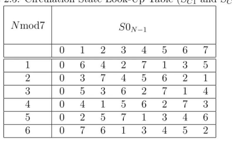
(44) Table 2.5: Circulation State Look-Up Table (SC1 and SC2 ) N mod7. 1 2 3 4 5 6. S0N −1 0 0 0 0 0 0 0. 1 6 3 5 4 2 7. 2 4 7 3 1 5 6. 3 2 4 6 5 7 1. 4 7 5 2 6 1 3. 5 1 6 7 2 3 4. 6 3 2 1 7 4 5. 7 5 1 4 3 6 2. Determination of CTC Circulation States [1] The state of the encoder is denoted S (0 ≤ S ≤ 7) with S = 4S1 + 2S2 + S3 , as shown in Fig. 2.8. The circulation states SC1 and SC2 are determined by the following operations: • Initialize the encoder with state 0. • Encode the sequence in the natural order for the determination of SC1 or in the interleaved order for determination of SC2 . Let the final state in each case be denoted S0N −1 . • According to the length N of the sequence, use Table 2.5 to find SC1 and SC2 .. 2.3.4. Subpacket Generation (Channel Interleaver or Interleaver and Puncturing) [1]. The proposed FEC structure punctures the mother codeword to generate a subpacket with various coding rates. The framework consists of the following: • bit separation,. 23.
(45) • subblock interleaving, • bit grouping, and • bit selection. The subpacket is also used in HARQ packet transmission. Figure 2.7 shows the block diagram of subpacket generation. A rate-1/3 CTC encoded codeword goes through interleaving and the puncturing. Figure 2.13 shows the block diagram of the interleaving block. The puncturing is performed to select a consecutive interleaved bit sequence that starts at some point of whole codeword. For the first transmission, the subpacket is generated to select the consecutive interleaved bit sequence that starts from the first bit of the systematic part of the mother codeword. The length of the subpacket is chosen according to the needed coding rate reflecting the channel condition. The first subpacket can also be used as a codeword with the needed coding rate for a burst where HARQ is not applied. Bit Separation All of the encoded bits can be demultiplexed into six subblocks denoted A, B, Y 1, Y 2, W 1, and W 2. The encoder output bits are sequentially distributed into the six subblocks with the first N bits going to the A subblock, the second N to the B subblock, the third N to the Y 1 subblock, the fourth N to the Y 2 subblock, the fifth N to the W 1 subblock, and the sixth N to the W 2 subblock. Subblock Interleaving The six subblocks can be interleaved separately. The interleaving is performed in unit of bits. The sequence of interleaver output bits for each subblock can be generated by the 24.
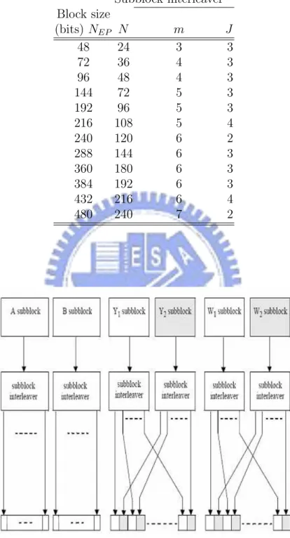
(46) procedure described below. The entire subblock of bits to be interleaved is written into an array at addresses from 0 to the number of the bits minus one (N − 1), and the interleaved bits are read out in a permuted order with the ith bit being read from the address ADi (i = 0, . . . , N − 1), as follows: 1. Determine the subblock interleaver parameters, m and J. Table 2.6 gives these parameters. 2. Initialize i and k to 0. 3. Form a tentative output address Tk according to Tk = 2m (k mod J) + BROm (bk/Jc). (2.16). where BROm (y) indicates the bit-reversed m-bit value of y (e.g.,BRO3 (6) = 3). 4. If Tk is less than N , ADi = Tk and increment i and k by 1. Otherwise, discard Tk and increment k only. 5. Repeat steps 3 and 4 until all N interleaver output addresses are obtained.. Bit Grouping The channel interleaver output sequence can consist of the interleaved A and B subblock sequences, followed by a bit-by-bit multiplexed sequence of the interleaved Y 1 and Y 2 subblock sequences, followed by a bit-by-bit multiplexed sequence of the interleaved W 1 and W 2 subblock sequences. The bit-by-bit multiplexed sequence of interleaved Y 1 and Y 2 subblock sequences can consist of the first output bit from the Y 1 subblock interleaver, the first output bit from the Y 2 subblock interleaver, the second output bit from the Y 1 subblock interleaver, the 25.
(47) Table 2.6: Parameters for the Subblock Interleavers Subblock interleaver Block size (bits) NEP 48 72 96 144 192 216 240 288 360 384 432 480. N 24 36 48 72 96 108 120 144 180 192 216 240. m 3 4 4 5 5 5 6 6 6 6 6 7. J 3 3 3 3 3 4 2 3 3 3 4 2. Figure 2.13: Block diagram of CTC channel interleaving scheme (from [1]).. 26.
(48) second output bit from the Y 2 subblock interleaver, etc. The bit-by-bit multiplexed sequence of interleaved W 1 and W 2 subblock sequences can consist of the first output bit from the W 1 subblock interleaver, the first output bit from the W 2 subblock interleaver, the second output bit from the W 1 subblock interleaver, the second output bit from the W 2 subblock interleaver, etc. Figure 2.13 shows the interleaving scheme. The order of bit grouping sequence is as follows: 0 A00 ,A01 ,...,A0N −1 ,B00 ,B10 ,...,BN −1 , 0 0 0 0 0 0 0 0 Y1,0 ,Y2,0 ,Y1,1 ,Y2,1 ,Y1,2 ,Y2,2 ,...,Y1,N −1 ,Y2,N −1 , 0 0 0 0 0 0 0 0 W1,0 ,W2,0 ,W1,1 ,W2,1 ,W1,2 ,W2,2 ,...,W1,N −1 ,W2,N −1 .. Bit Selection Lastly, bit selection is performed to generate the subpacket. The puncturing block is referred as bits selection in the viewpoint of subpacket generation. The mother code is transmitted with one of the subpackets. The bits in a subpacket are formed by selecting specific sequences of bits from the interleaved CTC encoder output sequence. The resulting subpacket sequence is a binary sequence of bits for the modulator. The parameters for bit selection are listed below: • k: the subpacket index when IR HARQ is enabled. – When IR HARQ is not used, k=0 (for the first transmission and increases by one for the next subpacket). – When there are more than one FEC block in a burst, the subpacket index for each FEC block shall be the same. • NEP : the number of bits in the encoder packet (before encoding).. 27.
(49) • NSCHk : the number of concatenated slots for the subpacket, as defined in [1, Table 569] for the non-HARQ and Chase HARQ CTC schemes. • mk : the modulation order for the kth subpacket (mk =2 for QPSK, 4 for 16-QAM, 6 for 64QAM). • SP IDk : the subpacket ID for the kth subpacket (for the first subpacket, SP IDk=0 =0). Also, let the scrambled and selected bits be numbered from zero with the 0th bit being the first bit in the sequence. Then, the index of the ith bit for the kth subpacket shall be Sk,i = (Fk + i)mod(3 · NEP ). (2.17). where i = 0, . . . , Lk −1, Lk = 48 ·NSCHk ·mk , and Fk = (SP IDk ·Lk )mod(3·NEP ). The NEP , NSCHk , mk , and SP ID values are determined by the base station (BS) and can be inferred by the subscriber station (SS) through the allocation size in the DL-MAP and UL-MAP. The above bit selection makes the following possible. • The first transmission includes the systematic part of the mother code. Thus it can be used as the codeword for a burst where the HARQ is not applied or when Chase HARQ is applied. • The location of the subpacket can be determined by the SP ID without the knowledge of previous subpacket. This is a very important property for IR HARQ retransmission. Note that the optional IR HARQ is not considered in our research, so we bypass a detailed introduction of the IR HARQ mechanism.. 28.
(50) Figure 2.14: Block diagram of a turbo decoder (from [11]).. 2.4 2.4.1. Decoding of CTC The Turbo Decoding Algorithm [11]. A key in turbo codes is the iterative decoding algorithm. In iterative decoding, the decoders for the constituent encoders take turns operating on the received data. Each decoder produces an estimate of the probabilities of the transmitted symbols; therefore, the decoders are soft output decoders. Probabilities of the symbols from one decoder, known as extrinsic probabilities, are interleaved and passed to the other decoder, where they are used as prior probabilities for the other decoder. The decoder thus passes probabilities back and forth between the decoders, with each decoder combining the evidence it receives from the incoming prior probabilities with the parity information provided by the code. After some number of iterations, hopefully the decoder converges to an estimate of the transmitted codeword. Since the output of one decoder is fed to the input of the next decoder, the decoding algorithm is called a turbo decoder, for it is reminiscent of turbo charging an automobile engine using engine-heated air at the air intake. Thus it is not really the code which is “turbo,” but rather the decoding algorithm which is “turbo.” The general operation of the turbo decoding algorithm is shown in Fig. 2.14.. 29.
(51) The MAP Decoding Algorithm [11], [13] One maximum a posteriori (MAP) decoding algorithm particularly suitable for estimating bit and/or state probabilities for a finite-state Markov system is the BCJR algorithm, named after Bahl, Cock, Jelinek, and Raviv who proposed it originally in 1974 [12]. While this algorithm has been known for some time, it was not extensively used for the decoding of convolutional codes because of the availability of a lower complexity Viterbi algorithm (for maximum-likelihood decoding of convolutional codes). In many respects, the BCJR algorithm is similar to the Viterbi algorithm. However, the conventional Viterbi algorithm computes hard decisions by outputting a single overall decision of the entire sequence of bits (or codeword) at the end, without providing the reliability of the decoder decisions on individual bits. Furthermore, the branch metric is based upon log likelihood values; no prior information is incorporated into the decoding process. The BCJR algorithm, on the other hand, computes soft outputs in the form of posterior probabilities for each message bit. While the Viterbi algorithm produces the maximum likelihood message sequence (or codeword), the BCJR algorithm produces the a posteriori most likely sequence of message bits, where the sequence of bits may not correspond to a continuous path through the trellis. The BCJR algorithm is a soft-input soft-output decoder that can be used directly in turbo decoding whereas the conventional Viterbi algorithm cannot without some modification to yield the required soft output. The BCJR algorithm for MAP decoding of convolutional codes consists of the following steps: • Compute branch metric γ. • Compute forward state metric α. • Compute backward state metric β.. 30.
(52) Figure 2.15: CTC trellis structure of duo-binary convolutional code with feedback encoder (from [14]). • Compute extrinsic log likelihood ratio Le . A more detailed understanding can be gained from [11].. 2.4.2. Decoding Rule for CRSC Codes with Non-binary Trellis [14]. The trellis of a double-binary feedback convolutional encoder has the structure shown in Fig. 2.15. The goal of the MAP algorithm is to provide us with Pr [dk = i|Observation] Pr [dk = 0|Observation] P(Sk−1 ,Sk ) p(Sk−1 , Sk , {yk }) d =i = ln P(Sk ,S ) , k−1 k p(S , S , {y }) k−1 k k dk =0. Li (dk ) = ln. i = 1, 2, 3,. (2.18). where yk is the received sample at time k. The index pair (Sk−1 , Sk ) determines the information symbol (bit couple) dk and the coded symbol xk from time k − 1 to time k where dk is in GF(22 ) with elements {0,1,2,3}. The sum of the joint probabilities p(Sk−1 , Sk , {yk }) in the numerator or in the denominator of (2.18) is taken over all labeled with dk = i, i = 0, 1, 2, 3, 31.
(53) where we have used decimal notation for dk instead of binary for convenience. With a memoryless transmission channel, the joint probability p(Sk−1 , Sk , {yk }) can be written as the product of three independent probabilities p(Sk−1 , Sk , {yk }) = p(Sk−1 , yj<k ) · p(Sk , yk |Sk−1 ) · p(yj>k , Sk ) , αk−1 (Sk−1 ) · γk (Sk−1 , Sk ) · βk (Sk ). (2.19). where yj<k denotes the sequence of received symbols yj from the beginning of the trellis up to time k − 1 and yj>k is the corresponding sequence from time k + 1 up to the end of the trellis. The forward recursion of the MAP algorithm yields αk (Sk ) =. X. αk−1 (Sk−1 ) · γk (Sk−1 , Sk ).. (2.20). Sk−1. The backward recursion yields βk−1 (Sk−1 ) =. X. γk (Sk−1 , Sk ) · βk (Sk ).. (2.21). Sk. When a transition between Sk−1 and Sk exists, the branch transition probability is given by γk (Sk−1 , Sk ) = p(Sk , yk |Sk−1 ) = p(Sk |Sk−1 ) · p(yk |Sk−1 , Sk ) = P (dk ) · p(yk |dk ).. (2.22). Let the natural logarithm of the branch transition probability metric be Γk (Sk−1 , Sk ) = ln γk (Sk−1 , Sk ). (2.23). and the natural logarithms of αk (Sk ) and βk (Sk ) be Ak (Sk ) = ln αk (Sk ) X = ln eAk−1 (Sk−1 )+Γk (Sk−1 ,Sk ) , Sk−1. 32. (2.24).
(54) Bk−1 (Sk−1 ) = ln βk−1 (Sk−1 ) X = ln eΓk (Sk−1 ,Sk )+Bk (Sk ) .. (2.25). Sk. Then the log-likelihood ratios (2.18) for i = 1, 2, 3 are given by P(Sk−1 ,Sk ) p(Sk−1 , Sk , {yk }) d =i Li (dk ) = ln P(Sk ,S ) k−1 k p(Sk−1 , Sk , {yk }) dk =0 P(Sk−1 ,Sk ) αk−1 (Sk−1 ) · γki (Sk−1 , Sk ) · βk (Sk ) d =i = ln P(Sk ,S ) k−1 k αk−1 (Sk−1 ) · γk0 (Sk−1 , Sk ) · βk (Sk ) dk =0 P(Sk−1 ,Sk ) A (S )+Γi (S ,S )+B (S ) e k−1 k−1 k k−1 k k k dk =i . = ln P(S ,S ) 0 k−1 k eAk−1 (Sk−1 )+Γk (Sk−1 ,Sk )+Bk (Sk ) dk =0. 2.4.3. (2.26). Simplified Max-Log-MAP Algorithm for Double-Binary CTC [14]. Implementing (2.26) in hardware is difficult and complex. It is also relatively complicated to implement it in DSP software. We consider the suboptimal max-log-MAP algorithm for double binary convolutional turbo codes. First, from (2.22) and (2.23), Γk (Sk−1 , Sk ) = ln γk (Sk−1 , Sk ) = ln[p(yk |dk ) · P (dk )].. (2.27). The distribution of the received symbols is given by, for i=0,1,2,3, p(yk |dk = i) = p(yks |xsk (i)) · p(ykp |xpk (i, Sk−1 , Sk )) = ·. 2 1 − Es [(y s,I −xs,I (i))2 +(yks,Q −xs,Q k (i)) ] e N0 k k π · N0 p,Q p,Q 2 2 1 − Es [(y p,I −xp,I k (i,Sk−1 ,Sk )) +(yk −xk (i,Sk−1 ,Sk )) ] e N0 k π · N0 s,I. = Ck · e0.5·Lc ·[yk. s,Q s,Q p,I p,I p,Q p,Q ·xs,I k (i)+yk ·xk (i)+yk ·xk (i,Sk−1 ,Sk )+yk ·xk (i,Sk−1 ,Sk )]. (2.28). where yks and ykp represent the received systematic and parity symbols, respectively, yks,I , yks,Q , ykp,I , and ykp,Q represent the received bit values transmitted through the I and Q channels, respectively, Lc = 4 · (fading factor) · (code rate) · 33. Eb N0. represent the channel reliability, and.
(55) s,Q 2 s,Q p,I 2 p,I p,Q 2 p,Q Es 2 2 2 2 −N [(yks,I )2 +(xs,I k (i)) +(yk ) +(xk (i)) +(yk ) +(xk (i,Sk−1 ,Sk )) +(yk ) +(xk (i,Sk−1 ,Sk )) ]. 1 )2 e Ck = ( π·N 0. 0. .. Hence, Γk (Sk−1 , Sk ) = ln[p(yk |dk ) · P (dk )] s,Q p,I p,I = 0.5 · Lc · [yks,I · xs,I · xs,Q k (i) + yk k (i) + yk · xk (i, Sk−1 , Sk ). + ykp,Q · xp,Q k (i, Sk−1 , Sk )] + ln P (dk ) + K. (2.29). where the constant K includes the constants and common terms that are cancelled in comparisons at later stages. Note that Ak (Sk ) = ln. X. eAk−1 (Sk−1 )+Γk (Sk−1 ,Sk ). Sk−1. ≈ max[Ak−1 (Sk−1 ) + Γk (Sk−1 , Sk )] Sk−1. Bk−1 (Sk−1 ) = ln. X. (2.30). eΓk (Sk−1 ,Sk )+Bk (Sk ). Sk. ≈ max[Γk (Sk−1 , Sk ) + Bk (Sk )] Sk. (2.31). The above can be derived by the Jacobian logarithm [11], i.e., ln(eL1 + eL2 ) = max(L1 , L2 ) + ln(1 + e−|L1 −L2 | ). (2.32). If the correction term (i.e., the second RHS term) is omitted and only the max term is retained, we obtain the above max-function (max-log-MAP) approximation. For iterative decoding of circular trellis, tail-biting gives A0 (S0 ) = AN (SN ) BN (SN ) = B0 (S0 ). ∀S0 ,. (2.33). ∀SN .. (2.34). As a result, the log-likelihood ratios (2.26) reduce to Li (dk ) ≈ −. max [Ak−1 (Sk−1 ) + Γik (Sk−1 , Sk ) + Bk (Sk )]. (Sk−1 ,Sk ). max [Ak−1 (Sk−1 ) + Γ0k (Sk−1 , Sk ) + Bk (Sk )].. (Sk−1 ,Sk ). 34. (2.35).
(56) We omit the detailed mathematical derivation for separating the log-likelihood ratios into intrinsic (prior information), systematic and extrinsic information. The interested reader may refer to [14]. It turns out that the extrinsic information can be expressed as s,Q Lei (dˆk ) = Li (dˆk ) − 0.5 · [yks,I · xs,I · xs,Q k (i) + yk k (i)] s,Q + 0.5 · [yks,I · xs,I · xs,Q k (0) + yk k (0)] − ln. P [dk = i] . P [dk = 0]. (2.36). The extrinsic information of the next decoder is computed from the prior information of previous decoder as Lai (dk ) = ln. P [dk = i] P [dk = 0]. (2.37). where i = 0, 1, 2, 3. Since a. a. P [dk = 01] = eL1 (dk ) · P [dk = 00], P [dk = 10] = eL2 (dk ) · P [dk = 00], a. P [dk = 11] = eL3 (dk ) · P [dk = 00], and P [dk = 00] + P [dk = 01] + P [dk = 10] + P [dk = 11] = 1, we have P [dk = 00] = P [dk = 10] =. 1. a a a 1+eL1 (dk ) +eL2 (dk ) +eL3 (dk ). La 2 (dk ) a a La (d ) 1+e 1 k +eL2 (dk ) +eL3 (dk ). , P [dk = 01] =. La 1 (dk ) a a La (d ) 1+e 1 k +eL2 (dk ) +eL3 (dk ). ,. , P [dk = 11] =. La 3 (dk ) a a La (d ) 1+e 1 k +eL2 (dk ) +eL3 (dk ). .. Using max-function approximation yields ln P [dk = 00] = − max[0, La1 (dk ), La2 (dk ), La3 (dk )], ln P [dk = 01] = La1 (dk ) − max[0, La1 (dk ), La2 (dk ), La3 (dk )], ln P [dk = 10] = La2 (dk ) − max[0, La1 (dk ), La2 (dk ), La3 (dk )], ln P [dk = 11] = La3 (dk ) − max[0, La1 (dk ), La2 (dk ), La3 (dk )]. Assuming equally likely symbols initially, we have A0 (S0 ) = 0 ∀S0 , BN (SN ) = 0 Lai (dk ) = 0 35. (2.38). ∀SN ,. (2.39). ∀i, dk .. (2.40).
(57) After sufficient decoding iterations, the decisions are made according to 01, = if L(dˆk ) = La1 (dk ) and La1 (dk ) > 0, 10, = if L(dˆk ) = La2 (dk ) and La2 (dk ) > 0, dˆk = a a ˆ 11, = if L(dk ) = L3 (dk ) and L3 (dk ) > 0, 00, = else,. (2.41). where L(dˆk ) = max[La1 (dk ), La2 (dk ), La3 (dk )]. This above algorithm have been known as the max-log-MAP algorithm which only uses the max functions to compute log-likelihood ratios. But coming with the approximation to reducing log-likelihood ratios is some performance degradation. We will see the effect later in the simulation results.. 36.
(58) Chapter 3 DSP Implementation Environment In our implementation, we employ the DSP baseboard SMT395 made by the Sundance company, which have a Texas Instruments (TI) TMS320C6416T DSP chip and a Xilinx Virtex-II Pro FPGA. In this chapter, we discuss the DSP system development environment, especially the VCP (Viterbi decoder coprocessor) and its features. The TI’s Code Composer Studio (CCS) EDMA and the 3L Diamond EDMA are also introduced.. 3.1. The DSP Baseboard. The DSP card used in our implementation is Sundance’s SMT395 shown in Fig. 3.1. It houses a 1 GHz 64-bit TMS320C6416T DSP of TI. The SMT395 is supported by TI’s Code Composer Studio and the 3L Diamond real-time operating system (RTOS) to enable multiDSP system implementation with minimum effort by the programmer. Features of the SMT395 board include: • 1 GHz TMS320C6416T fixed-point DSP processor with L1 and L2 cache that has 8000 MIPS peak DSP performance. • Xilinx Virtex II Pro FPGA XC2VP30-6 in FF896 package.. 37.
(59) Figure 3.1: Sundance’s SMT395 module (from [18]). • 256 Mbytes of SDRAM at 133 MHz. • Eight 2 Gbit/sec Rocket Serial Links (RSL) for inter module communication. • Two Sundance High-Speed Bus (50MHz, 100MHz or 200MHz) ports at 32 bits width. • 8 Mbytes flash ROM for configuration and booting.. 3.2. The Viterbi-Decoder Coprocessor (VCP) [19]. The Viterbi-decoder coprocessor (VCP) is on some of the number of the TMS320C6000 DSP family, including C6416, C6418, and C6455. It has been designed to perform Viterbi decoding for IS2000 and 3GPP wireless standards. We can also use it for other convolutional decoding applications, including WiMAX.. 3.2.1. Overview of VCP [19], [21], [22]. The VCP should be accessed using the EDMA (Enhanced Direct Memory Access) for mostly, but the CPU must first configure the VCP control values. There are also a number of 38.
(60) Figure 3.2: VCP block diagram (modified from [19]). functions available to the CPU to monitor the VCP status and access decision and output parameter data. The DSP controls the operation of the VCP using memory-mapped registers and data buffers. The DSP typically sends and receives data using synchronized EDMA transfer through the 64-bit EDMA bus. The VCP sends two synchronization events to the EDMA: a receiver event (VCPREVT) and a transmit event (VCPXEVT), as shown in Fig. 3.2. The VCP is composed of VCP Control, EDMA I/F unit, memory block, processing unit, CPU interrupt generator, and REVT/XEVT generator. Fig. 3.2 shows two VCP external communication mechanisms, in one of which DSP (CPU) accesses VCP Control through the 32-bit peripheral bus and in the other EDMA I/F unit through the 64-bit EDMA bus. In the latter case, EDMA channel 28 (RX) is for V CP transmission to DSP and EDMA channel 29 (TX) is for DSP transmission to V CP . Fig. 3.3 and Fig. 3.4 show the DSP chip architecture and chip die photo, where the. 39.
(61) Figure 3.3: DSP chip architecture (from [20]).. Figure 3.4: DSP chip die (from [20]).. 40.
(62) position of the VCP is indicated. The VCP input data are the branch metrics and the output data are the hard or soft decisions. The VCP provides the following features and capabilities: • Variable constraint length, K = 5, 6, 7, or 9. • User-supplied code coefficients. • Code rate (1/2, 1/3, or 1/4). • Configurable trace back settings (convergence distance, frame structure). • Branch metrics calculation and depuncturing is done in software by the DSP. • Frees up DSP resources for other processing. • Communication between the DSP and the VCP is performed through a high performance DMA engine. • VCP uses its own optimized working memories. The VCP is able to decode only a subset of the convolutional codes known as single register, nonrecursive convolutional codes (an example is shown in Fig. 3.5). Important parameters for this type of codes are: • The constraint length K (K = the number of linear finite-state registers + 1). • The rate R is given by R = k/n, where k is the number of information bits needed to produce n output bits known as the codeword. • The generator polynomials Gn describe how the outputs are generated from the inputs.. 41.
(63) Figure 3.5: Convolutional encoder example, where K = 3, R = 1/3, G0 = (100)8 , G1 = (101)8 , G2 = (111)8 (from [19]). From the parameters, we can derive a trellis diagram providing a useful representation of the code whose complexity grows exponentially with the constraint length K. Fig. 3.6 shows the trellis diagram of the code of Fig. 3.5. As a maximum-likelihood sequence estimation (MLSE) decoder, the Viterbi decoder identifies the code sequence with the highest probability of matching the transmitted sequence based on the received sequence. The Viterbi algorithm is composed of a metric update and a traceback routine. The metric update performs a forward recursion in the trellis over a finite number of symbol periods where probabilities are accumulated (the VCP accumulates on 12 bits) for each individual state based on the current input symbol (branch metric information). Once a path through the trellis is identified, the traceback routine performs a backward recursion in the trellis and outputs hard or soft decisions. To facilitate the decoding process, the initial state of delay elements is all zero. In addition, by appending (K − 1) zero tail bits at the end of the F -bit input sequence, it is. 42.
(64) Figure 3.6: Convolutional code trellis example (from [19]). also ensured that the final state is the all-zero state, which is called zero tail. For example, in Fig. 3.7 the decoded sequence is uest = 0,1,1,1 and the last four zeros in the path are tail bits and not part of the information frame (F ). As IEEE 802.16e CC adopts tail-biting, we used to modify the basic way of using VCP to handle it.. 3.2.2. VCP Inputs (Brach Metrics and VCP Input Configuration) [19], [22]. BM (Branch Metrics) are calculated by the DSP and stored in the DSP memory subsystem as 7-bit signed values. For rate 1/n codes, a total of 2n−1 branch metrics need to be computed per symbol period and passed to the VCP. Consider BPSK modulated bits (0 → 1, 1 → −1), for example. Let the rate be 1/2. Then there are 2 branch metrics per symbol period. We have BM0 (t) = r0 (t) + r1 (t),. 43.
(65) Figure 3.7: Example of survivor path and associated decoded sequence (from [21]). Table 3.1: Branch Metrics for Rate-1/2 Code Address (hex) Base Base + 4h Base + 8h. MSB. LSB. BM1 (t = T ) BM0 (t = T ) BM1 (t = 0) BM0 (t = 0) BM1 (t = 3T ) BM0 (t = 3T ) BM1 (t = 2T ) BM0 (t = 2T ) ........... BM1 (t) = r0 (t) − r1 (t), where r(t) is the received codeword at time t. Note that if we utilize the VCP to decode CC, we must note the definition of the VCP modulation. We find that it may reverse the index of the constellation coordinate for three different modulations. The data should be sent to the VCP as described in Table 3.1 for rate-1/2 coding (the base address must be double-word aligned). For rate-1/3 and 1/4 coding, the interested reader may refer to [19] for details. The branch metrics can be saved in the DSP memory subsystem in either their native format or packed in words by the user. By default, the VCP works in the little-endian mode, but it can also work in the big-endian, whose detailed settings are discussed in [19]. VCP Input FIFO (Brach Metrics) The FIFO is used in a double-buffering fashion as shown in Fig. 3.8. The VCP generates a VCPXEVT synchronization event each time the top half or bottom half of the buffier is 44.
數據
![Figure 2.15: CTC trellis structure of duo-binary convolutional code with feedback encoder (from [14]).](https://thumb-ap.123doks.com/thumbv2/9libinfo/8004521.160153/52.892.277.605.158.459/figure-ctc-trellis-structure-binary-convolutional-feedback-encoder.webp)

+7
![Figure 3.4: DSP chip die (from [20]).](https://thumb-ap.123doks.com/thumbv2/9libinfo/8004521.160153/61.892.230.657.468.930/figure-dsp-chip-die-from.webp)
![Figure 3.13: VCP frame, reliability, and convergence length limitations(modified from [19])](https://thumb-ap.123doks.com/thumbv2/9libinfo/8004521.160153/71.892.192.696.162.339/figure-vcp-frame-reliability-convergence-length-limitations-modified.webp)
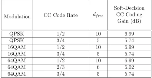
相關文件
It’s (between/next to) the church and the
Listen - Check the right picture striped hat polka dotted hat.. Which hat do
Play - Let’s make a big family How many people are in your family1. Write it
Sam: I scraped my knee and bumped my head.. Smith: What happened
straight brown hair dark brown eyes What does he look like!. He has short
While Korean kids are learning how to ski and snowboard in the snow, Australian kids are learning how to surf and water-ski at the beach3. Some children never play in the snow
I am writing this letter because I want to make a new friend in another country.. Maybe you will come to Gibraltar
Sam: It’s really nice, but don’t you think it’s too expensive.. John: Yeah, I’m not going to buy it, but I wish I could
