一個用於無線網路中找出最小權重獨立控制集的多項式時間近似方案

國 立 交 通 大 學

應用數學系

碩 士 論 文

一個用於無線網路中找出最小權重

獨立控制集的多項式時間近似方案

A Polynomial-time Approximation Scheme for the

Minimum-weighted Independent Dominating Set

Problem in Wireless Networks

研 究 生：吳思賢

指導教授：陳秋媛 教授

一個用於無線網路中找出最小權重

獨立控制集的多項式時間近似方案

A Polynomial-time Approximation Scheme for the

Minimum-weighted Independent Dominating Set

Problem in Wireless Networks

研 究 生：吳思賢 Student：Sih-Sian Wu

指導教授：陳秋媛 Advisor：Chiuyuan Chen

國 立 交 通 大 學

應 用 數 學 系

碩 士 論 文

A Thesis

Submitted to Department of Applied Mathematics

College of Science

National Chiao Tung University

in Partial Fulfillment of the Requirements

for the Degree of

Master

in

Applied Mathematics

June 2010

Hsinchu, Taiwan, Republic of China

i

一個用於無線網路中找出最小權重獨立控制集的

多項式時間近似方案

研究生：吳思賢

指導老師：陳秋媛 教授

國 立 交 通 大 學

應 用 數 學 系

摘 要

在無線網路中，每一個節點的能力不一定相同，例如，電池的剩餘電量不一定相 同，訊息傳遞所需的花費不一定相同，因此，一個常見的方式是利用點權重圖（也 就是將無線網路所對應的圖的點加上權重）來描述網路的拓樸結構。一個點權重 圖的最小權重獨立控制集，指的是一組既是獨立集也是控制集的最小權重點集 合。在本論文中，我們針對具有多項式成長有界性質的點權重圖提出一個計算最 小權重獨立控制集的多項式時間近似方案；具有多項式成長有界性質的圖包含了 著名的單位圓盤圖、單位圓球圖、和類單位圓盤圖。就我們所知，我們的多項式 時間近似方案是第一個針對無線網路中最小權重獨立控制集問題的多項式時間 近似方案。此外，當所有點的權重都一樣時，我們的多項式時間近似方案會是一 個在具有多項式成長有界性質的圖中計算獨立控制集的多項式時間近似方案；值 得一提的是：我們的多項式時間近似方案只需要一個階段，因此簡化了Hurink和 Nieberg在文獻[15]中所提出需要兩個階段的多項式時間近似方案。 關鍵詞：控制集，獨立控制集，最小權重獨立控制集，近似演算法，多項式時間 近似方案。 中 華 民 國 九 十 九 年 六 月

A polynomial-time approximation scheme for the

minimum-weighted independent dominating set

problem in wireless networks

Student: Sih-Sian Wu Advisor: Chiuyuan Chen

Department of Applied Mathematics National Chiao Tung University

Abstract

Due to different capabilities of nodes (for example, different remaining battery lives or dif-ferent costs for transmitting a message) in a wireless network, it is desirable to model the underlying network topology by a node-weighted graph. A minimum-weighted indepen-dent dominating set of a node-weighted graph is a vertex subset with the minimum weight being both independent and dominating. In this thesis, we present a polynomial-time ap-proximation scheme (PTAS) for computing a minimum-weighted independent dominating set in a node-weighted polynomially growth bounded graph, which is in a class of graphs that include the well-known unit disk graphs, unit ball graphs, and quasi unit disk graphs. To the best of our knowledge, our PTAS is the first PTAS for the minimum-weighted inde-pendent dominating set problem in wireless networks. Furthermore, when all the weights are identical, our PTAS turns out to be a simple 1-stage PTAS for computing an inde-pendent dominating set in a polynomially growth bounded graph and hence simplifies the 2-stage PTAS proposed by Hurink and Nieberg in [15].

Key words: Dominating set; Independent dominating set; Minimum-weighted

independent dominating set; Approximation algorithms; Polynomial-time approximation scheme.

iii

誌謝

能完成這篇畢業論文，最需要感謝的就是我的指導教授–陳秋媛

教授。在我遇到瓶頸的時候，老師總是有耐心地教導我，給我一個正

確的方向，這讓我的研究能順利地完成。老師對我的照顧不僅止於課

業上，老師也時常關心我的生活，讓我能無憂無慮的進行研究。

再來我要感謝的是國元學長，學長幫助我完成了整篇論文的架構，

還有給我數據模擬的方向。對於我的問題，學長也總是不厭其煩地回

答我。我真的非常感謝學長這兩年來的指導。

要感謝的人很多，不管是最會解決問題的鈺傑學長，還是時常跟

我一起討論問題的思綸、健峰，還有在我做研究苦悶時，一起打球的

同學，真的很謝謝大家在我研究所這段期間的幫忙。

Contents

Abstract (in Chinese) i Abstract (in English) ii Acknowledgement iii

Contents iv

List of Figures v

1 Introduction 1

1.1 Minimum independent dominating set problem . . . 1 1.2 Minimum-weighted independent dominating set problem . . . 2 1.3 Our result . . . 3 2 Preliminaries 4 2.1 polynomially growth bounded graphs . . . 4 2.2 Terminologies . . . 4 3 A PTAS for the MWIDS problem on node-weighted polynomially growth

bounded graphs 6

4 Comparing our PTAS with HN PTAS 10 5 Concluding remarks 12

List of Figures

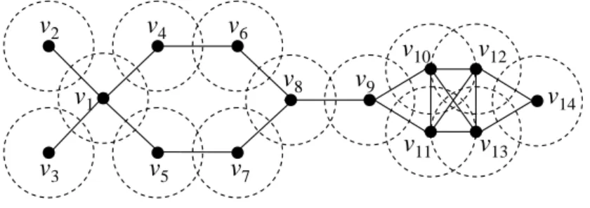
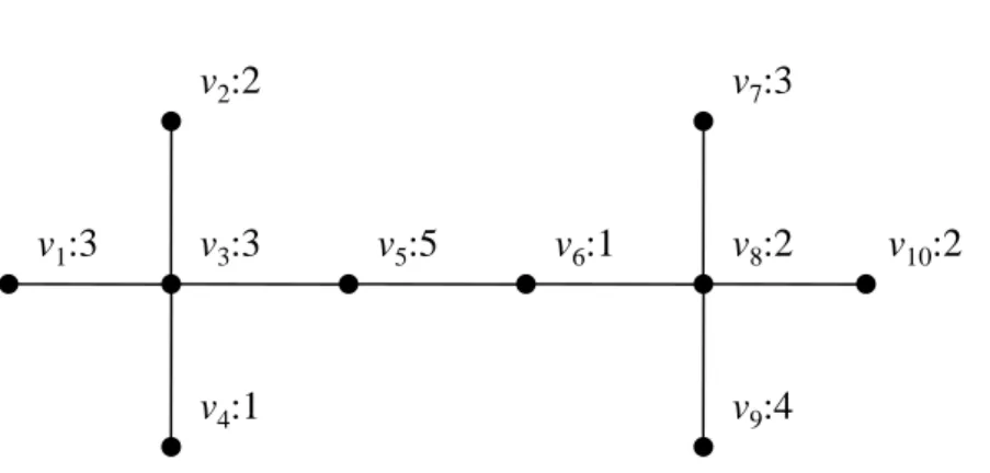
1 A unit disk graph. . . 3 2 An example of node-weighted graph with Wopt = {v3, v8} and wopt = 5. . . 5

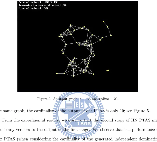
3 An input graph; ε = 1.5 and radius = 20. . . 11 4 An output of HN PTAS when ε = 1.5 and radius = 20: (a) after stage 1,

(b) after stage 2. . . 12 5 An output of our PTAS when ε = 1.5 and radius = 20. . . 12 6 Comparing the cardinality of independent dominating set when ε = 1.5

and radius = 15. . . 13 7 Comparing the cardinality of independent dominating set when ε = 1.5

and radius = 20. . . 13 8 A comparison on successful ratio of algorithm in case ε =1.5, radius = 15. 14 9 A comparison on successful ratio of algorithm in case ε =1.5, radius = 20. 14

1. Introduction

1.1. Minimum independent dominating set problem

Most works on optimization problems that arise in wireless networks model networks by graphs. In this thesis, graphs refer to simple undirected graphs. Let G = (V, E) be a graph with vertex set V and edge set E. A subset I of V is an independent set if no two vertices in I are adjacent. A subset D of V is a dominating set if every vertex in V \ D has a neighbor in D. The following two problems have been extensively studied in the literature: the Maximum Independent Set Problem (MIS) and the Minimum Dominating Set Problem (MDS). The former asks for finding an independent set with the maximum cardinality and the latter, finding a dominating set with the minimum cardinality. Since the above two problems have been extensively studied in the literature [5, 6, 7, 9, 11, 12, 13, 16, 17, 18], the Minimum Independent Dominating Set Problem (MIDS), which is to find a subset of vertices that is both an independent and a dominating set with the smallest cardinality, has received much attention in the literature [2, 9, 15, 19]. A maximal independent set is an independent set that is not a subset of any other independent set. It is well-known that any independent dominating set is a maximal independent set, and vice versa. Therefore, MIDS is also known as the Minimum Maximal Independent Set Problem.

It has been proven that MIDS is N P -complete in general graphs [12]. Furthermore, Halld´orsson [13] showed that MIDS in general graphs can not be approximated within the ratio n1−ε unless P = N P . In addition, MIDS remains N P -complete under strict restrictions: for example, for bipartite graphs and comparability graphs [7], for planar graphs, triangle-free graphs and claw-free graphs [2], for line graphs [20], and for 2P3-free

graphs [19]. On the other hand, MIDS can be solved in polynomial time for chordal graphs [9], cocomparability graphs [16], and asteroidal triple-free graphs [3]. In [15], Hurink and Nieberg presented a 2-stage polynomial-time approximation scheme (PTAS)

for MIDS in polynomially growth bounded graphs. For more details, see [2, 19]. 1.2. Minimum-weighted independent dominating set problem

In real world applications, nodes in a wireless network usually have different capabil-ities (for example, different remaining battery lives or different costs for transmitting a message). Therefore, in this thesis we assume there are positive weights on vertices of a graph and we call such a graph a node-weighted graph. For convenience, a vertex of a graph is also called a node. The Minimum-Weighted Independent Dominating Set Prob-lem (MWIDS) is to find an independent dominating set Ω of a node-weighted graph such that the sum of weights of nodes in Ω is minimized. MWIDS is clearly a generalization of MIDS since the latter can be reduced to the former by letting all nodes have the same positive weight.

In this thesis, we mainly concern with MWIDS in node-weighted polynomially growth bounded graphs. The class of polynomially growth bounded graphs includes most of the graphs used to model wireless networks such as Unit Disk Graphs, Quasi Unit Disk Graphs, Unit Ball Graphs, and Coverage Area Graphs [15, 17], where a Unit Disk Graph (UDG) is defined as the intersection graph of equal radius disks in the Euclidean plane (see Figure 1). Since MIDS is a special case of MWIDS and MIDS is N P -complete in general graphs, it follows that MWIDS is N P -complete in general graphs. Chang [4] showed that MWIDS is N P -complete for chordal graphs. Farber presented a linear time algorithm to locate a minimum weight independent dominating set in a chordal graph with 0-1 vertex weights [9], which is a bit different from the original MWIDS problem. Farber et al. also used polynomial time to deal with MWIDS in permutation graphs [11] and strongly chordal graphs [10].

For node-weighted polynomially growth bounded graphs, many researchers considered the Minimum-Weighted Dominating Set Problem (MWDS) and the Minimum-Weighted Connected Dominating Set Problem (MWCDS); see [1, 8, 14, 21, 22]. Till now, the best

v₁ v₄ v₅ v₆ v₇ v₂ v₃ v₁₄ v₁₂ v₁₀ v₉ v₁₃ v₁₁ v₈

Figure 1: A unit disk graph.

known approximation ratios for MWDS and MWCDS in UDGs are obtined by Zou et al. in [22]; they presented a (4 + approximation algorithm for MWDS and a (5 + ε)-approximation algorithm for MWCDS in UDGs. To the best of our knowledge, there is no related result for MWIDS in polynomially growth bounded graphs in the literature. 1.3. Our result

In this thesis, we present a PTAS for MWIDS in a subclass of node-weighted poly-nomially growth bounded graphs. In particular, we prove that if the weight function of a node-weighted graph satisfies the following weight-constraint, then there exists a PTAS for MWIDS.

Weight-constraint: There exists a constant t > 0 such that for every pair u, v of nodes of a node-weighted graph G, w(u) ≤ t · w(v) holds.

This constraint is reasonable in real world applications as, for example, the difference between the remaining battery lives of any two nodes or the difference between the costs for transmitting a message from any two nodes cannot be unbounded. Do notice that by assigning the same weight to every node, our PTAS turns out to be a simple 1-stage PTAS for MIDS in polynomially growth bounded graphs and hence simplifies the 2-stage PTAS proposed by Hurink and Nieberg in [15]. For convenience, we call the PTAS proposed by Hurink and Nieberg in [15] HN PTAS in the remaining sections.

This thesis is organized as follows: Section 2 gives the preliminaries including the definitions and terminologies. We present our PTAS for MWIDS in polynomially growth

bounded graphs in Section 3. A comparison between Our PTAS with HN PTAS are given in Section 4. Concluding remarks are given in Section 5.

2. Preliminaries

polynomially growth bounded

2.1. polynomially growth bounded graphs

For any two vertices u and v of G, let d(u, v) denote the number of hops in a shortest path from u to v. The following definitions are crucial in this thesis. The r-neighborhood of v, denoted by Nr[v], is defined by

Nr[v] = {u ∈ V | d(u, v) ≤ r}.

So, N0[v] = {v} and N1[v] is the set of v and the neighbors of v. For convenience, let

N [v] = N1[v]. Analogously, for a subset U of V , let N [U ] =

S

u∈U N [u]. The following

definition is given by Hurink and Nieberg [15].

Definition 1. Let G = (V, E) be a graph. If there exists a function f (·) such that every r-neighborhood in G contains at most f (r) independent vertices, then G is f -growth-bounded. Furthermore, we say that G has polynomially bouuded growth is for some constant c ≥ 1, f (r) is bounded by a polynomial of maximal degree c, i.e., f (r) = O(rc).

In [15], Hurink and Nieberg mentioned that the growth function f (·) does not depend on the number of vertices in the given graph, but on the radius of the neighborhoods only. For example, a UDG has p(r) = (2r + 1)2 = O(r2); see [18].

2.2. Terminologies

For a given optimization problem, an algorithm is called a ρ-approximation algorithm for some ρ ≥ 1 if it always returns a feasible solution of relative error no more than ρ. Here ρ is called the approximation ratio and the solution derived is called a ρ-approximation.

For a given optimization problem, an algorithm is called a polynomial-time approximation scheme (PTAS) if it is an approximation algorithm that takes as input not only an instance of the problem but also a value ε > 0 such that it is a (1 + ε)-approximation algorithm and for any fixed ε > 0, it runs in time polynomial in the size n of its input instance.

In the remaining discussion, we assume that G = (V, E) is a node-weighted p-growth-bounded graph where p(·) is a polynomial function, and n is used to denote the number of vertices of G. For a subset U of V , the subgraph induced by U is denoted by G[U ]. Let Wopt be a minimum-weighted independent dominating set of G and wopt be the weight

of Wopt, where the weight of a vertex subset is the sum of weights of all vertices in this

subset. For a subset of vertices U of G, define W∗(U ) to be a function that returns a minimum-weighted independent dominating set for U in G. We denote w∗(U ) to be the weight of W∗(U ). Note that W∗(U ) is always computed with respect to the entire graph G which is updated after an iteration of algorithm; therefore, the set returned by W∗(U ) may contain vertices outside U (but the set returned by W∗(U ) is always contained in N [U ]). For example, consider in Figure 2. Suppose all nodes have the same weight. Then W∗({v1, v2}) = {v3} 6⊆ {v1, v2}, but W∗({v1, v2}) ⊆ N [{v1, v2}]. Clearly,

Wopt = W∗(V ) and wopt = w∗(V ).

v₁:3 v₂:2 v₄:1 v₃:3 v₅:5 v₆:1 v₇:3 v₈:2 v₁₀:2 v₉:4 ID:Weight

Figure 2: An example of node-weighted graph with Wopt= {v3, v8} and wopt= 5.

A d-separated collection is a collection {S1, S2, . . . , Sk}, where Si ⊆ V, i = 1, 2, . . . , k,

subgraphs induced by subsets in a d-separated collection divide the original graph into smaller parts so that it becomes easier to solve a given optimization problem. In [18], Nieberg and Hurink successfully used a 2-separated collection to derive a PTAS for MDS in polynomially growth bounded graphs. They also used the same idea to derive a PTAS for MIDS in polynomially growth bounded graphs in [15].

3. A PTAS for the MWIDS problem on node-weighted polynomially growth bounded graphs

In order to present our PTAS, we first propose statement (1) and Lemma 3.1. For v ∈ V , let Ir[v] denote a maximum independent set of Nr[v]. Since a maximum independent

set is also a dominating set, we have

| W∗(Nr[v]) | ≤ | Ir[v] | ≤ p(r). (1)

The following lemma says that obtaining an optimal solution W∗(Nr[v]) for Nr[v] can

be done in polynomial time if r is bounded.

Lemma 3.1. Let G = (V, E) be a node-weighted graph. Then for any neighborhood Nr[v],

we can obtain W∗(Nr[v]) in nO(p(r)) time.

Proof. By statement 1, we know the cardinality of W∗(Nr[v]) is at most p(r). It becomes

clear that we can obtain W∗(Nr[v]) in nO(p(r)) time.

Before going further, we need two lemmas.

Lemma 3.2. Let G = (V, E) be a node-weighted graph. For a d-separated collection {S1, S2, . . . , Sk}, where Si ⊆ V, i = 1, 2, . . . , k, in G with d ≥ 2, we have

wopt ≥Pk_i=1 w∗(Si).

Proof. For each subset Si ⊆ V , consider the neighborhood N [Si]. By definition, N [Si]

Pk

i=1 w(Wopt∩ N [Si]). Since Wopt∩ N [Si] dominates Si and is independent in G, we have

w(Wopt∩ N [Si]) ≥ w∗(Si). This implies

wopt ≥Pk_i=1 w(Wopt∩ N [Si]) ≥Pk_i=1 w∗(Si).

Lemma 3.3. Let {S1, S2, . . . , Sk} be a d-separated collection in a node-weighted graph

G = (V, E), d ≥ 2, and let T1, T2, . . . , Tk be subsets of V with Si ⊆ Ti for all i = 1, 2, . . . , k.

If there exists a bound ρ ≥ 1 such that w∗(Ti) ≤ ρ · w∗(Si) holds for all i = 1, 2, . . . , k,

then Pk i=1 w ∗_(T i) ≤ ρ · wopt. Moreover, ifSk i=1 W ∗_(T

i) is a minimum-weighted independent dominating set of G, then

it is a ρ-approximation of a minimum-weighted independent dominating set of G. Proof. This lemma follows from

Pk

i=1 w ∗_(T

i) ≤Pk_i=1ρ · w∗(Si) ≤ ρ · wopt.

We now are ready to introduce our PTAS; it is presented in Algorithm 1.

Our PTAS works as follows. Initially, set the independent dominating set Ω to be the empty set. Start with an arbitrary vertex v ∈ V and consider the r-neighborhood Nr[v], for r = 0, 1, 2, and so on. For each r, compute minimum-weighted independent

dominating sets for the neighborhoods Nr+2[v] and Nr[v] and compute their total weight

whenever

w∗(Nr+2[v]) > (1 + ε) · w∗(Nr[v]).

After stopping increasing the radius r of the neighborhoods, the desired bound on the weight of an independent dominating set is obtained. Update Ω and update the remaining vertices. Repeat the above process until V is empty.

Algorithm 1 An algorithm for the MWIDS problem.

Input: a node-weighted polynomially growth bounded graph G = (V, E) and a constant ε > 0

Output: an independent dominating set Ω of G which is a (1 + ε)-approximation for the MWIDS problem

1: _{Ω = ∅; i = 0;} 2: _{while V 6= ∅ do}

3: i = i + 1; . the i-th iteration

4: Pick v ∈ V ; 5: r = 0; 6: while w∗(Nr+2[v]) > (1 + ε) · w∗(Nr[v]) do 7: r = r + 1; 8: end while 9: Ω = Ω ∪ W∗(Nr+2[v]); 10: V = V \ N [W∗(Nr+2[v])]; 11: end while 12: return Ω;

We now analyze Algorithm 1. First of all, the following lemma shows that the radius of the largest neighborhood we need to examine for each vertex picked in line 3 of Algorithm 1 is bounded by a constant that only depends on the growth function p and the given constant ε. In other words, the number of iterations of the inner while-loop is constant. Lemma 3.4. Let G = (V, E) be a node-weighted p-growth-bounded graph and the weight function satisfies the weight-constraint. Then for the i-th iteration of Algorithm 1, there exists a constant c (only depends on ε) such that the number of iterations in lines 6-8 is at most c.

Proof. Let the growth function p be p(r) = O(rd) for some constant d ≥ 1. Consider a vertex v picked in line 3 in the i-th iteration of Algorithm 1. Let ˆr denote the first r which violates the inequality in line 6. Now we consider any value r < ˆr. Let v∗ be the vertex in Nr+2[v] with the maximum weight. If r is even, then by (1), we have

p(r + 2) · w(v∗) ≥ w∗(Nr+2[v]) > (1 + ε) · w∗(Nr[v]) .. . > (1 + ε)r2+1· w∗(N₀[v]) = (1 + ε)r2+1· w(x), for some x ∈ N [v].

Recall that there exists a constant t > 0 such that for every pair of vertices u, v in G, w(u) ≤ t · w(v) holds. Hence we have (1 + ε)r2+1 < t · p(r + 2) = O((r + 2)d); this inequality will be violated for some large enough r. Therefore, there must exist a constant c (which depends on ε) such that r ≤ c holds. Similar arguments can be applied for odd r.

Theorem 3.5. Algorithm 1 is a PTAS with approximation ratio (1 + ε) for the MWIDS problem on node-weighted polynomially growth bounded graphs G = (V, E) if the weight function satisfies the weight-constraint.

Proof. We first prove that Algorithm 1 generates a minimum-weighted independent dom-inating set with approximation ratio (1 + ε). Suppose at the end of Algorithm 1, the value of i is k; that is, suppose there are total k iterations of the while-loop in lines 2-11. For each i, let vi be the vertex picked in line 3 and let ri be the radius which is the first value

violating the inequality in line 6. Then we have w∗(Nri+2[vi]) ≤ (1 + ε) · w

∗

(Nri[vi]). (2) Let Si = Nri[vi] and Ti = Nri+2[vi] for i = 1, 2, . . . , k. It is not difficult to verify that S = {S1, S2, . . . , Sk} forms a 2-separated collection. Clearly, Si ⊆ Ti. By (2), w∗(Ti) ≤

(1 + ε) · w∗(Si) holds for all i = 1, 2, . . . , k. By Lemma 3.3,

Pk i=1w ∗_(T i) ≤ (1 + ε) · wopt. Algorithm 1 returns Ω =Sk i=1W ∗_(T

i). If we can further prove that Ω is an independent

dominating set of G, then by Lemma 3.3, Ω is a (1 + ε)-approximation for a minimum-weighted independent dominating set of G. Ω is a dominating set of G since in the i-iteration, the removed neighborhood N [W∗(Nri+2[vi])] is dominated by W

∗_(T

i). Ω is an

independent set of G since for each i, W∗(Ti) is independent and if there exist two vertices

a, b with a ∈ W∗(Ti), b ∈ W∗(Tj), for some i 6= j, then b 6∈ N [W∗(Ti)] and a 6∈ N [W∗(Tj)]

and therefore W∗(Ti) ∪ W∗(Tj) is also independent. From the above discussion, Ω is a

(1 + ε)-approximation of a minimum-weighted independent dominating set of G.

by a constant c = c(ε). It has been shown in [15] and [18] that c(ε) = O(1_εlog1_ε). By Lemma 3.1, for each i, finding each of the local optimal solutions W∗(N0[vi]), W∗(N1[vi]),

. . ., W∗(Nri+2[vi]) can be done in polynomial time n

O(1_εlog1_ε)_{. Thus the total execution}

time spent on line 6 is bounded by a polynomial in n. Since the overall running time of Algorithm 1 is dominated by the total execution time spent on line 6, Algorithm 1 takes polynomial time.

4. Comparing our PTAS with HN PTAS

To compare our PTAS with HN PTAS, we vary the number of nodes n from 50 to 100 with the increment of 10 and for each n, we generate one hundred unit disk graphs (UDGs). The method to generate a UDG with n nodes is to randomly place n nodes in a square of area size 100 × 100m2_{. If the distance between any two nodes is within 1, there}

is an edge between them. It is well known that UDGs are polynomially growth bounded graphs.

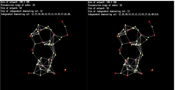
HN PTAS [15] is a 2-stage algorithm; see Algorithm 2 and Algorithm 3 in Appendix. If the output of the first stage is not an independent set, then the second stage will be initiated in order to deal with those dependent vertices. The second stage will remove non-independent vertices from the output of first stage and adds independent ones by using maximal independent set scheme on vertices which have not been dominated. We implement our PTAS and HN PTAS by using the C programming language. See Figures 3, 4 and 5 for an example. Note that the vertices colored red in Figures 4 and 5 are the vertices in the output (i.e., the independent dominating set).

From Figure 4(a), we know that the first stage of HN PTAS produces 12 vertices and two of them are dependent. Thus the second stage of HN PTAS is initiated to tackle the problem; one of the two dependent vertices is removed and two vertices are added to the output; see Figure 4(b). The cardinality of the output of HN PTAS is therefore 13. For

Figure 3: An input graph; ε = 1.5 and radius = 20.

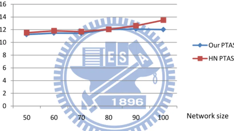
the same graph, the cardinality of the output of our PTAS is only 10; see Figure 5. From the experimental results, we observe that the second stage of HN PTAS may add many vertices to the output of the first stage. We observe that the performance of our PTAS (when considering the cardinality of the generated independent dominating set) outperforms that of HN PTAS; see Figures 6 and 7.

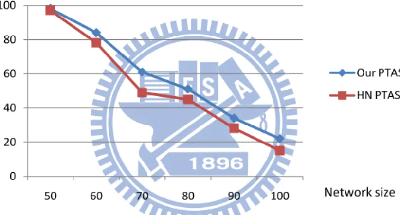
Note that both our PTAS and HN PTAS need to use brute force to obtain local optimal solutions. Since the local area that our PTAS needs to apply the brute force method is always no greater than that of HN PTAS, it is clear that our PTAS is more efficient than HN PTAS. But, how efficient? We give a threshold of 10 seconds, meaning that if a brute force execution exceeds 10 seconds, then the corresponding graph will be removed from the experimental set. From Figures 8 and 9, we see that the successful ratio (the ratio of graphs that do not exceed the threshold of 10 seconds) of our PTAS outperforms that of HN PTAS.

Figure 4: An output of HN PTAS when ε = 1.5 and radius = 20: (a) after stage 1, (b) after stage 2.

Figure 5: An output of our PTAS when ε = 1.5 and radius = 20.

5. Concluding remarks

In this thesis, we consider the minimum-weighted independent dominating set problem on node-weighted polynomially growth bounded graphs. We have proven that if the weight function satisfies the weight-constraint: for every pair u, v of vertices, there exists a constant t > 0 such that w(u) ≤ t · w(v) holds, then our algorithm is a PTAS for

15 15.5 16 16.5 17 17.5 18 18.5 19 19.5 20 50 60 70 80 90 100 Our PTAS HN PTAS Cardinality Network size

Figure 6: Comparing the cardinality of independent dominating set when ε = 1.5 and radius = 15.

0 2 4 6 8 10 12 14 16 50 60 70 80 90 100 Our PTAS HN PTAS Cardinality Network size

Figure 7: Comparing the cardinality of independent dominating set when ε = 1.5 and radius = 20.

the MWIDS problem on node-weighted polynomially growth bounded graphs. To the best of our knowledge, this is the first result for the MWIDS problem. Our PTAS has approximation ratio (1+ε) and it can be done in polynomial time nO(1εlog

1

ε). Our algorithm can also be used to solve the minimum independent dominating set problem.

0 20 40 60 80 100 50 60 70 80 90 100 Our PTAS HN PTAS Successful ratio(%) Network size

Figure 8: A comparison on successful ratio of algorithm in case ε =1.5, radius = 15.

0 20 40 60 80 100 50 60 70 80 90 100 Our PTAS HN PTAS Network size Successful ratio(%)

Figure 9: A comparison on successful ratio of algorithm in case ε =1.5, radius = 20.

References

[1] Ambuhl, C., Erlebach, T., Mihalak, M., Nunkesser, M., 2006. Constant-factor ap-proximation for minimum-weight (connect) dominating sets in unit disk graphs. In: Lecture Notes in Computer Science 4110. pp. 3–14.

[2] Boliac, R., Lozin, V., 2003. Independent domination in finitely defined classes of graphs. Theoretical Computer Science 301 (1-3), 271–284.

[3] Broersma, H., Kloks, T., Kratsch, D., M¨uller, H., 1999. Independent sets in asteroidal triple-free graphs. SIAM Journal on Discrete Mathematics 12 (2), 276–287.

[4] Chang, G., 2004. The weighted independent domination problem is NP-complete for chordal graphs. Discrete Applied Mathematics 143 (1-3), 351–352.

[5] Chang, M., 1998. Efficient algorithms for the domination problems on interval and circular-arc graphs. SIAM Journal on Computing 27 (6), 1671–1694.

[6] Cheng, X., Huang, X., Li, D., Wu, W., Du, D., 2003. A polynomial-time approxima-tion scheme for the minimum-connected dominating set in ad hoc wireless networks. Networks 42 (4), 202–208.

[7] Corneil, D., Perl, Y., 1984. Clustering and domination in perfect graphs. Discrete Applied Mathematics 9 (1), 27–39.

[8] Dai, D., Yu, C., 2009. A 5 + ε-approximation algorithm for minimum weighted dom-inating set in unit disk graph. Theoretical Computer Science 410 (8-10), 756–765. [9] Farber, M., 1982. Independent domination in chordal graphs. Operations Research

Letters 1 (4), 134–138.

[10] Farber, M., 1984. Domination, independent domination, and duality in strongly chordal graphs. Discrete Applied Mathematics 7 (2), 115–130.

[11] Farber, M., Keil, J. M., 1985. Domination in permutation graphs. Journal of Algo-rithms 6 (3), 309–321.

[12] Garey, M. R., Johnson, D. S., 1979. Computers and Intractability: A Guide to the Theory of NP-Completeness. W. H. Freeman & Co., New York, NY, USA.

[13] Halld´orsson, M. M., 1993. Approximating the minimum maximal independence num-ber. Information Processing Letters 46 (4), 169–172.

[14] Huang, Y., Gao, X., Zhang, Z., Wu, W., 2008. A better constant-factor approx-imation for weighted dominating set in unit disk graph. Journal of Combination Optimization 18 (2), 179–194.

[15] Hurink, J. L., Nieberg, T., 2008. Approximating minimum independent dominating sets in wireless networks. Information Processing Letters 109 (2), 155–160.

[16] Kratsch, D., Stewart, L., 1993. Domination on cocomparability graphs. SIAM Journal on Discrete Mathematics 6 (3), 400–417.

[17] Nieberg, T., Hurink, J., 2004. Wireless communication graphs. In: Palaniswami, M and Krishnamachari, B and Challa, S (Ed.), Proceedings of the 2004 Intelligent Sensors, Sensor Networks & Information Processing Conference. pp. 367–372, Intel-ligent Sensors, Sensor Networks and Information Processing Conference, Melbourne, Australia, Dec. 14-17, 2004.

[18] Nieberg, T., Hurink, J., 2006. A PTAS for the minimum dominating set problem in unit disk graphs. Vol. 3879 of Lecture Notes in Computer Science. pp. 296–306, 3rd International Workshop on Approxination and Online Algorithms, Palma de Mallorca, Spain, Oct. 06-07, 2005.

[19] Orlovich, Y. L., Gordon, V. S., de Werra, D., 2009. On the inapproximability of independent domination in 2P3-free perfect graphs. Theoretical Computer Science

410 (8-10), 977–982.

[20] Yannakakis, M., Gavril, F., 1980. Edge dominating sets in graphs. SIAM Journal on Applied Mathematics 38 (3), 364–372.

[21] Zou, F., Li, X., Gao, S., Wu, W., 2009. Node-weighted steiner tree approximation in unit disk graphs. Journal of Combination Optimization.

[22] Zou, F., Wang, Y., Xu, X.-H., Li, Du, H., Wan, P., Wu, W., 2009. New approxi-mations for minimum-weighted dominating sets and minimum-weighted connected dominating sets on unit disk graphs. Theoretical Computer Science.

6. Appendix

Algorithm 2 The first stage of HN PTAS.

Input: G = (V, E) polynomially growth bounded graph ε > 0 Output: Dominating set ¯D

1: _{D = ∅; i = 0;}¯ 2: _{while V 6= ∅ do} 3: Pick v ∈ V ; 4: ri = 0;

5: while D(i)_ri+3(v) > (1 + ε) · Dr(i)i (v) do

6: ri = ri+ 1;

7: end while

8: Color vertices in D_r(i)_i+3(v) with color i;

9: D = ¯¯ D ∪ D_r(i)_i+3(v);

10: V = V \ Γri+3(v);

11: i = i + 1;

12: end while

Algorithm 3 The second stage of HN PTAS. Input: G = (V, E), Dominating set ¯D, v ∈ ¯D

1: Assert that v is conflicting;

2: D = ¯¯ D \ {v};

3: V0 = V \ Γ( ¯D);

4: Compute maximal independent set I on G[V0];

19 //File Name: PTAS_for_MIDS.cpp

//Author: 吳思賢

//Email Address: smallhau@gmail.com

//Description: This program is a PTAS (polynomial-time approximation scheme) // for the minimum independent dominating set problem on unit disk graphs. //Input: One hundred adjacency matrices; each matrix represents a unit disk // graph and the entries of each matrix are generated randomly.

//Output: The average cardinality and the average execution time for generating // the independent dominating sets of the one hundred unit disk graphs.

#include <stdio.h> #include <stdlib.h> #include <iostream> #include <fstream> #include <time.h> #include <cstdlib> using namespace std;

#define NETWORK_SIZE 50 //設定 NETWORK 的 size.

int check(int adj[ ][NETWORK_SIZE+1], int IDS[ ], int N[ ], int nb_size, int size); //目的：利用 adjacency matrix adj 來判斷所選的點集 IDS 是否真的是

// an independent dominating set of a given r-Neighborhood N. //需給傳入值的參數：adj, IDS, N, id, size

//需做傳出值的參數：無

//傳回：1 表示判斷之結果為"是"；0 表示判斷之結果為"否". //參數 adj：存放 unit disk graph 的 adjacency matrix.

//參數 IDS：存放某個選進的點集, 以便判斷是否為 local independent dominating set.

//參數 N：存放 r-Neighborhood 中的所有點. //參數 nb_size：存放 r-Neighborhood 的 size. //參數 size：被選進點集的 size.

int Neib( int node, int r, int adj[ ][NETWORK_SIZE+1], int N[ ], int wb[ ]); //目的：找尋點 node 的 r-Neighborhood.

//需給傳入值的參數：node, r, adj, wb //需做傳出值的參數：N

20 //傳回：node 的 r-Neighborhood 的 size.

//參數 node：由 node 這點出發, 找尋這點的 r-Neighborhood. //參數 r：同 check 函數. //參數 adj：同 check 函數. //參數 N：同 check 函數. //參數 wb：當某點已經被其他點控制時, 在找尋 neighborhood 的時候, 就不需要 // 考慮該點, wb 就是用來記錄各個點是否已經被控制了. // wb 是 1 表示已經被控制, wb 是 0 表示尚未被控制.

void bruteforce(int node, int r, int adj[ ][NETWORK_SIZE+1], int IDS[ ], int N[ ], int wb[ ], int &size);

//目的：以暴力法求出點 node 的 r-Neighborhood 的 minimum independent // dominating set (MIDS)以及此 MIDS 的 size.

//此 function 會呼叫 function Neib 及 function check //需給傳入值的參數：node, r, adj, N, wb

//需做傳出值的參數： IDS, size //參數 node：同 Neib 函數. //參數 r：同 check 函數. //參數 adj：同 check 函數.

//此外 node 的 r-Neighborhood 的 MIDS 也用參數 IDS 傳出

//參數 IDS：若某個點集經由 function check 判斷出是 local independent // dominating set, 則此點集將由 IDS 傳出.

//參數 N：同 check 函數. //參數 wb：同 Neib 函數.

//參數 size：點 node 的 r-Neighborhood 的 MIDS 的 size, 此值將傳出.

int GRAPH_num = 100; //設定跑 100 張圖.

int radius = 10; //點跟點之間距離小於 radius, 就會產生邊.

double epsi = 1.5; //設定 PATS 中的誤差 epsi.

int threshold = 10; //設定單次演算法執行時間假如超過 10 秒, 即結束此回合.

int main(void) {

time_t t1, t2;

time(&t1); //將初始時間存進 t1 變數.

int first, i, j, k, r, node, id, round; int wb[NETWORK_SIZE];

21

int size, size2; //存放 local independent dominating set 的 size. FILE* fptr; char temp; char filename[7]; char output[40]; sprintf(output, "V_epsi=%.1f_radius=%d_size=%d_thresh=%d.txt", epsi,radius,NETWORK_SIZE,threshold);

int total_cardi = 0; //最後 independent dominating set 的 size. //wb[NETWORK_SIZE] 紀錄各個點是否已經被控制了. ofstream outf; outf.open(output,ios::out); //以下步驟是執行 100 次不同圖的演算法 for(round = 1; round <= GRAPH_num; round++) {

int adj[NETWORK_SIZE][NETWORK_SIZE+1]; //記錄圖的連接矩陣. int N2[NETWORK_SIZE]; //記錄點的(r+2)-Neighborhood. int N[NETWORK_SIZE]; //紀錄點的 r-Neighborhood.

int omega[NETWORK_SIZE]; //記錄我們求出的 independent //dominating set.

sprintf(filename, "%d.txt", round+ GRAPH_num); fptr = fopen( filename, "r");

//以下步驟是以二維連接矩陣存取圖的結構. for ( i = 0; i < NETWORK_SIZE; i++ ) {

wb[i] = 0;

for ( j = 0; j < NETWORK_SIZE+1; j++ ) {

temp = fgetc( fptr ); adj[i][j] = atoi( &temp ); }

}

22

int index = 0;

//以下步驟是從 id 小的點去判斷該點是否已被控制. for(i = 0; i < NETWORK_SIZE; i++)

{ if (!wb[i]) //假如該點還沒被控制 { int Nr_IDS[NETWORK_SIZE]; int Nrtwo_IDS[NETWORK_SIZE]; node = i; r = 0; //以下步驟為執行演算法內的 while 迴圈. do {

bruteforce(node, r+2, adj, Nrtwo_IDS, N2, wb, size2); bruteforce(node, r, adj, Nr_IDS, N, wb, size);

r = r+1; } while(size2 > (1+epsi)*size); if (!size2) { index = 0; break; }

size2 = size2 + index;

//以下步驟是將選定的點存進 omega 矩陣, //並將那些被 omega 矩陣控制的點標為 1. for(j = index; j < size2; j++) {

omega[j] = Nrtwo_IDS[j-index]; wb[omega[j]] = 1;

23 if(adj[k][omega[j]]) wb[k] = 1; } index = size2; } }

total_cardi = total_cardi + index;

}

(void) time(&t2); //記錄演算法的終止時間.

//以下為 output 我們所求出的 the average cardinality of independent //dominating set 和整個程式的執行時間.

outf<<(float)total_cardi/ GRAPH_num <<endl; outf<<(int)t2-t1<<"s"<<endl;

outf.close( );

system("pause"); return 0;

}

int check(int adj[ ][NETWORK_SIZE+1], int IDS[ ], int N[ ], int nb_size, int s) {

int i, j, flag;

//以下步驟是 check 選進的點集 IDS 是否 independent for(i = 0; i < s-1; i++)

for(j = i+1; j < s; j++)

if(adj[IDS [i]][ IDS [j]]) return 0;

//以下步驟是 check 選進的點集 IDS 是否為控制集 for(i = 0; i < nb_size; i++) {

24 flag = 0;

for( j = 0; j < s; j++) {

if((IDS [j] == N[i]) || (adj[N[i]][ IDS [j]] == 1)) { flag = 1; break; } } if (!flag) return 0; } return 1; }

int Neib(int node, int r, int adj[ ][NETWORK_SIZE+1], int N[ ], int wb[ ]) { int id = 1; int current = 1; int i,j,k,temp; int node_wb[NETWORK_SIZE]; N[0] = node; //以下步驟是以 node_wb 矩陣存取該點是否被選過, 避免重複選到 for(i = 0; i < NETWORK_SIZE; i++)

node_wb[i] = 0;

node_wb[node] = 1;

//以下步驟求出 1-Neighborhood

for(i = 0; i < NETWORK_SIZE; i++) {

if (((adj[N[0]][i]) && (!node_wb[i])) && (!wb[i])) {

25 N[id] = i; node_wb[i] = 1; id++; } } //以下步驟求出 r-Neighborhood for(k = 1; k < r; k++) { temp = id;

for(j = current; j < temp ; j++) {

for(i = 0; i < NETWORK_SIZE; i++) {

if (((adj[N[j]][i]) && (!node_wb[i])) && (!wb[i])) { N[id] = i; node_wb[i] = 1; id++; } } } current = temp; } return id; }

void bruteforce(int node, int r, int adj[ ][NETWORK_SIZE+1], int IDS[ ], int N[ ], int wb[ ], int &size) {

int first, i, s, nb_size; time_t t3, t4;

(void) time(&t3); //記錄此暴力法的初始時間. int b[NETWORK_SIZE];

26 nb_size = Neib(node,r,adj,N,wb); if (nb_size == 1) { IDS[0] = N[0]; size = 1; return; } //以下步驟以暴力法求出最佳解. for(s = 1; s < nb_size; s++) { (void) time(&t4); //記錄此時時間. //以下步驟是判斷執行時間是否超過 10 秒,假如超過就回傳 0. if ((int)t4-t3 > threshold) { size = 0; return ; } int flag = 0; for( i = 0; i < s; i++) { b[i] = i; IDS[i] = N[i]; }

if (check(adj, IDS, N, nb_size, s)) { size = s; return; } while(!flag) {

27 flag = 1;

for( i = s-1; i >= 0; i--) {

if (b[i] != (nb_size – s + i)) { first = i; flag = 0; break; } } if (!flag) { b[first] = b[first]+1; IDS [first] = N[b[first]];

for( i = first+1; i < s; i++) {

b[i] = b[i-1]+1; IDS [i] = N[b[i]]; }

if (check(adj, IDS, N, nb_size, s)) { size = s; return; } } } } }