TeV到PeV能區的微中子天文學

國

立 交 通 大 學

物

理

研

究

所

碩

士

論

文

TeV到PeV能區的微中子天文學

Neutrino Astronomy in the TeV to PeV Energy Range

研

究 生 ： 董念恩

指

導 教 授 ：

林貴林教授

TeV到PeV能區的微中子天文學

Neutrino Astronomy in the TeV to PeV Energy Range

研

究

生 ： 董念恩

_{Student: Nien-En Tung}

指

導 教 授 ：

林貴林教授

_{Advisor: Prof. Guey-Lin Lin}

國

立 交 通 大 學

物

理

研

究

所

碩 士

論 文

A Thesis

Submitted to Institute of Physics

National Chiao Tung University

in Partial Fulfillment of the Requirements

for the Degree of

Master of Physics

in

June, 2007

Hsinchu City, Taiwan, Republic of China

中華民國九十六年六月

Neutrino Astronomy in the TeV to PeV Energy Range

Student: Nien-En Tung

Advisor: Prof. Guey-Lin Lin

Institute of Physics

National Chiao Tung University

ABSTRACT

We examine the prompt and conventional atmospheric neutrino fluxes where dif-ferent models for the prompt flux are employed. Due to difdif-ferent angular depen-dencies between the prompt flux and the conventional ones, we compare the shower event ratio due to the prompt flux to that due to the conventional flux. This is important to separate the prompt atmospheric neutrino flux from the conventional component. The determination of the former is useful for testing the models for charm productions.

Acknowledgements

Contents

Abstract i

Acknowledgements ii

Contents iii

List of Tables v

List of Figures vii

1 Introduction 1

1.1 Primary Flux . . . 2

1.2 The Property of Neutrinos . . . 2

1.3 The Gamma Ray Burst . . . 5

2 The Primary Cosmic Ray Flux 6 2.1 Atmosphere Model . . . 6

2.2 The Cascade Equations for Cosmic Ray Interactions . . . 7

2.3 Analytic Solutions to Cascade Equations . . . 9

3 Shower Event Rates 15 3.1 Primary Cosmic Ray model . . . 15 3.2 Conventional and Prompt Neutrino Flux . . . 16 3.3 Shower Events . . . 23 3.4 Numerical Results on Shower Events Rates and Angular Dependencies 24

List of Tables

3.1 Parameters for Eq. (3.1) . . . 16

3.2 Parameters for νe from K decay . . . 18

3.3 Particles data . . . 19

3.4 RQPM ZN M parameters . . . 20

3.5 The branching ratio of decays channel. . . 21

3.6 Decay Z moments for charm and K. . . 22

4.1 Ec = 1.0 × 105 GeV, 10 years of data taking. R=0.12 for conven-tional ν’s . . . 33

4.2 Ec = 2.5 × 105 GeV, 10 years of data taking. R=0.11 for conven-tional ν’s . . . 33

4.3 Ec = 5.0 × 105 GeV, 10 years of data taking. R=0.10 for conven-tional ν’s . . . 33

4.4 Ec = 1.0 × 105 GeV, 10 years of data taking. R=0.13 for conven-tional ν’s . . . 34

4.5 Ec = 2.5 × 105 GeV, 10 years of data taking. R=0.11 for conven-tional ν’s . . . 34

4.6 Ec = 5.0 × 105 GeV, 10 years of data taking. R=0.10 for

List of Figures

3.1 Primary flux weighted by E2_{. The solid line for power law, red cross}

for Honda’s fitting and blue square for Eq. (3.2). . . 17 3.2 Charm Z-moment for PQCD, considering the primary either with

or without a knee, as a function of energy [1]. . . 21 3.3 Cross section for νN interactions at high energies according to

CTEQ4-DIS parton distribution [2]. . . 25 3.4 The comparison of electron neutrino fluxes given by different

mod-els. The y-axis is the weighted flux spectra and x-axis is the neutrino energy in GeV unit. This is for the zenith angle 0◦_{. . . 26}

3.5 This shows the electron neutrino flux in the horizontal direction. The intersection of conventional and prompt fluxes locates around 106 _{GeV due to the enhancement of the conventional flux in the}

3.6 Event number spectra for three years of data-taking in km3 _water

Cherenkov detector. The black lines are conventional shower events. The solid one is shower events from the low zenith angle bin θ = [0◦_{, 60}◦_{]. The dashed one is shower events from the high zenith angle}

bin θ = [60◦_{, 90}◦_{]. The colored lines are prompt and GRB(red)}

shower events. The prompt and GRB shower event are isotropic. The magenta line means RQPM-SV model for shower events. The blue and green lines represent the RQPM-FS and PQCD models for shower events respectively. . . 28 3.7 Ratio versus energy threshold Ec. The black curve represents the

ratio for the conventional flux. The flux ratio including contribu-tions of the prompt flux is represented by the dotted color line. According to different charm production models used to calculate the prompt flux, the magenta, blue and green dotted lines represent total flux ratios where the prompt component of the flux is cal-culated by RQPM-SV, RQPM-FS ans PQCD models respectively. The solid color lines denote flux ratios with the GRB neutrino flux also added into the total flux. . . 30

Chapter 1

Introduction

In TeV to PeV range of cosmic rays, prompt atmospheric neutrino flux increas-ingly dominates the conventional background and becomes more important. To probe the footprint of neutrinos, one must record its EM and hadronic shower events. The significant difference of prompt flux and the conventional one is the angular dependence. We use the angular difference in integrated shower event rate to separate the prompt flux from the conventional one.

This thesis is organized as follows. In Chapter 1 we review relative physics background. We show basic properties of cascade equations in Chapter 2. We also show the main numerical results for shower events and the integrated event rate for different prompt models. In Chapter 4, we summarize important facts.

1.1

Primary Flux

The charged cosmic rays from outer space consist of 86% protons, 11% α-particles, 1% nuclei of heavier elements up to uranium, and electrons. These elements come from the primary source, and other components such like positrons and antiprotons are believed from interstellar gas. Neutral particle consists of γ-ray , neutrino and antineutrino.

The chemical proportions of these components are constant with energy, while the flux often has energy dependence. For primary cosmic rays, it is described by inverse power law energy spectrum

φ ∝ E−(γ+1). (1.1)

Discontinuation in the power law index is the main physical characteristic of cosmic rays. There is the first break called ‘knee’ around 106 _{GeV. Below the}

knee, the spectrum has power law E−2.7 _{dependence, steepening to E}−3.0 _above

the knee. The other break called ‘ankle’ locates at about 109 _{GeV. These breaks}

reflect the different acceleration mechanisms in the sources of high energy cosmic particles.

1.2

The Property of Neutrinos

Neutrinos were first postulated in 1930 by Pauli to explain abnormal phenomena from β-decay. At that time β-decay was regarded as a two-body decay

n → p++ e−_{. (1.2)}

The outgoing energy of particles from two-body system can be determined kinematically and the escaping electron is monochromatic. The energy was assumed to be E = (m 2 n− m2p + m2e m2_n )c 2_{. (1.3)}

But experimentally it showed that the outgoing electron has an energy distribu-tion.

The above formula only determines the maximal outgoing energy. To solve this puzzle, Pauli proposed a new particle which is called ‘neutrino’ by Fermi and he used this three-body model to explain the electron energy distribution. He predicted that the new particle is neutral in charge and has very a small mass. Then the correct description of β-decay is

n → p++ e−_{+ ¯ν (1.4)}

In 1956, Clyde Cowan and Frederick Reines confirmed the existence of neutrino experimentally.

Neutrinos interact with other matter by the to weak force, which can be classified into two kinds. One is called neutral current; the other is called charge current. Neutral current process interchanges the Z boson. Charge current involves W+ _{and W}−_{. The mediators Z and W}± _{have masses 92 GeV and 82}

GeV respectively.

Neutral current process, such as νl + X → νl + Y , has no other matter

annihilated or created and the neutrino only gains or loses its energy. Therefore, neutral current process is an elastic scattering.

In the charge current process, there is an exchange of neural and charged leptons. The reaction is νl+ X → l + Y , and the incoming νl, which interacts

with the proton, can results in the creation of a charge lepton l.

Neutrinos at low energy have less chance to interact with other matters due to small cross section. For example, in the reaction ¯νe+ e− → ¯νµ+ µ− ,the cross

section is σ(¯νe+ e−→ ¯νµ+ µ−) ∝ α2 (s − m2 W)2 . (1.5) When s ≪ m2

W, the approximation gives

σ ∼ α

2_s

m4 W

∼ G2F, (1.6)

where GF is Fermi constant. Approximately the numerical result of the cross

1.3

The Gamma Ray Burst

Gamma-ray bursts (GRBs) are the most luminous events known in the universe. GRBs often last from milliseconds to a few seconds which is followed by emission at longer wavelengths in X-rays or radio spectrum. One possible explanation for the mechanism of GRB is the relativistic expanding fireball model, powered by radiation pressure [3] [4].

The cosmic ray above 1011 _{GeV is most likely dominated by an extra-galactic}

source of protons. High energy neutrino production is associated with the produc-tion of high energy protons, through the decay of charged pion which is produced by interactions of accelerated proton with fireball photon via the process

p + γ → ∆ → n + π+. (1.7) GRBs and active galactic nuclei (AGN) jets have been suggested as possible sources of high energy neutrino associated high energy cosmic rays. Based on the constrain of total energy power of 1010 _{GeV to 10}12 _{GeV, Waxman and Bahcall}

set the cosmic upper bound for the neutrino flux [5]. We use their model as extra-galactic neutrino sources.

Chapter 2

The Primary Cosmic Ray Flux

2.1

Atmosphere Model

The atmospheric neutrino flux depends on the model for the atmosphere. In studying the propagation of particles, an important quantity is called slant depth which is the total substance mass from the top of atmosphere downward the position of the incoming particle over unit area. Slant depth is defined as

X = Z ∞

l

ρ(l, θ)dx, (2.1)

where ρ(l, θ) is the atmospheric density at the altitude h(l, θ). If we ignore the curvature of the Earth, we can approximated h(l, θ) as follows

h(l, θ) ≃ l cos θ + l

2

2Rsin

2_{θ, (2.2)}

where R is the radius of the Earth. This expression is a good approximation for zenith angle less than 60◦_{. We adopt the simple isothermal model for the density}

of the atmosphere,

ρ(l, θ) = ρ0exp(−

h h0

), (2.3)

with scale height h0 and X0 = ρ0h0 = 1030 g/cm2.

2.2

The Cascade Equations for Cosmic Ray

In-teractions

The cosmic particle interacts with the nucleons of atmosphere and these inter-actions cause the energy change of the incoming particle. Let us take X to be the slant depth, and φ(E, X) the flux density of particles at energy E and slant depth X. In the differential layer (X, X + dX), one defines the growth ratio of the flux density as is dp ≡ dφφ. The basic description of the change in the number

of primary nucleons is dp dX = −α(E) + β(E, X). (2.4) In other words, dφ φ dX = −α(E) + β(E, X), (2.5) where α(E) means the flux reduction due to the interactions; β(E, X) is the gain term. β(E, X) is also represented as β(E, X) = S(E,X)_φ(E,X), where S(E, X) is the source term about high energy nucleons contributing to the number of lower energy. Primary particles of lower energy state are only produced from all possible of higher energy ones. Therefore, the source term is

S(E, X) = Z ∞

E

φ(E′_{, X)α(E}′_)F

N N(E′, E) dE′, (2.6)

where FN N is the dimensionless cross section [6]. F (E′, E) means the chance of

energy E′ _{state turning to the energy E state . The term α(E) is ρσ(E), where}

ρ is volume density of target nucleons, and σ(E) is the cross section. _α(E)1 is also defined as interaction length λ(E), which means the average slant depth of the occurrence of interaction. Some authors assume that λ(E) slightly depends on E. In this work, we treat λ(E) for nucleon as a constant [6].

The production of mesons mainly comes from the interaction of primary cosmic flux with the substances of atmosphere. Those mesons, such as π, K, and D mesons, are unstable and with short lifetimes. The cascade equation for describing the flux of meson is

dφM(E, X) dX = −( 1 λM + 1 λd )φM + Z ∞ E φN(E′, X)BN MFN M(E′, E) λN(E′) dE′_{, (2.7)}

where λM is the interaction of mesons and λd is the decay length which equals to

γρ(E, X)d0. γ is time dilation factor and d0 is decay length in vacuum. Meson

has a gain in number from the high energy primary nucleon flux. Different from the cascade equation of the primary flux, the formula for meson has an additional decay term resulting in the reduction of the meson flux.

The mesons are the source of atmospheric neutrino flux via the weak decay. The evolution equation for lepton flux is

dφl(E, X) dX = − 1 λl φl+ Z ∞ E φM(E′, X)BM lFM l(E′, E) λd(E′) dE′_{, (2.8)}

the interaction length of neutrino is much longer than atmosphere depth. Therefore the interaction term can be ignored and the equation only contains the contribution from meson flux .

2.3

Analytic Solutions to Cascade Equations

It is possible to solve cascade equation by using three approximations: (i) cosmic ray flux φ(E, X) can be factorized into the form A(E)B(X); (ii) the interaction length is independent of energy; (iii) the source term is assumed to follow the Feynman scaling [6] [7].

First of all, without any approximation, we have: dφN(E, X) dX = − 1 λN φN(E, X) + Z ∞ E φN(E′, X)FN M(E′, E) λ(E′₎ dE ′ , (2.9) dφM(E, X) dX = −( 1 λM + 1 λd )φM + Z ∞ E φN(E′, X)BN MFN M(E′, E) λN dE′_{, (2.10)} dφl(E, X) dX = − 1 λl φl+ Z ∞ E φM(E′, X)BM lFM l(E′, E) λd dE′, (2.11) where the integration forms are source terms.

dχ(X) χ(X)dX = − 1 λN + 1 λN 1 N(E)GN N(E), (2.12) with GN N(E) = Z ∞ E N(E′)FN N(E′, E) dE′, (2.13)

where λN is a constant according to assumption (ii). If we define _Λ1_N = _χ(X)dXdχ(X) ,

then the solution of χ(X) can be

χ(X) = χ(0) exp(−_ΛX

N

). (2.14)

The flux diminishes exponentially when going through the atmosphere with atten-uation length ΛN.

From the observed data, we can assume N(E) has a power law energy behavior N(E) = E−(γ+1)_{, and we apply Feynman scaling F (E}′_{, E) =} 1

EF ( E E′) to the source term [6] [7]. Let x = E E′, then GN N(E) = Z ∞ E N(E′_)F N N(E′, E) dE = N(E) Z 1 0 N(x)FN N(x)x−2dx, And we define ZN N as ZN N = Z 1 0 xγ−1FN N(x) dx. (2.15)

It is a γ-dependent constant under the assumption of Feynman-scaling. The constant is called Z-moment. Z-moments may have energy dependence if one dose not assume Feynman-scaling and factorization of particle flux. From Eq. (2.12) and Eq. (2.14), the attenuation length ΛN satisfies the following relation:

1 ΛN = 1 λN + ZN N λN . (2.16)

Due to meson decays and interactions, the meson flux ray be expressed by Eq. (2.10), where λd is the function of X or E . Although we could obtain

φM(E, X) by numerical computation, we choose to solve it approximately based

upon certain physical arguments.

Assuming that the present energy of meson is greater than its critical energy, then the interaction term is dominant because meson decay length is longer the than interaction length. This situation is called high energy approximation. By neglecting the decay term λd, Eq. (2.10) turns into

dφM(E, X) dX = − 1 λM φM + Z ∞ E φN(E′, X)BN MFN M(E′, E) λN dE′_{, (2.17)}

The meson flux satisfies boundary condition φM(E, 0) = 0 since secondary

the cosmic rays must be produced from the interaction of primary flux with atmosphere matters. Also, we can use separation of variables and scaling of source terms to obtain the solution for the meson flux. Assuming that φM(E, X) = M(E)χM(X) and M(E) has the same power law form as N(E) [7].

dχM(X) χM(X)dX = − 1 λM + 1 λN ZN M(E). (2.18)

With the boundary condition φM(E, 0) = 0, the solution is

φM(E, X) = N0E−(γ+1)( ZN M 1 − ZN N )( λM λM − ΛN)(exp(− 1 λM) − exp(− 1 λN )). (2.19) To obtain the low energy (E ≪ ǫM) approximation, we use integration factor and

deduce the exact solution

φM(E, X) = N0E−(γ+1)exp(− X ΛM )ZN M λN Z X 0 (X ′ X) ǫM E cos θ exp(X ′ λM − X′ ΛN ) dX′_, (2.20) For E ≪ ǫM, (X ′ X) ǫM

E cos θ is approaching to zero unless X′ is close to X. Using

X′

→ X as the low energy situation, one can show that φM(E, X) = N0E−(γ+1) Z_λN MN exp(− X ΛN)λd(E) = N0E−(γ+1) Z_1−ZN MN N 1 ΛN exp(− X ΛN), (2.21) For E ≫ ǫM, (X ′ X) ǫM

E cos θ is close to 1 and the formula can be reduced to Eq.

(2.19) [7].

Therefore, by integrating Eq. (2.11), the neutrino flux from the low energy meson is given by φν = ZM ν ZN M 1 − ZN N(1 − exp(− X ΛN ))N0E−(γ+1), (2.22)

φν = ZM ν

ZN M

1 − ZN N

N0E−(γ+1). (2.23)

This has no angular dependence. Similarly, the high energy flux at the ground level is φν = ZM ν ZN M 1 − ZN N ( λM λM − ΛN ) ln (λM ΛN ) ǫM cos θN0E −(γ+2)_{. (2.24)}

for high energy result, the flux has maximum at the horizon. But Eq. (2.24) has singularity at θ = 0◦_{. In fact, this expression is valid only for θ < 60}◦ _{and for}

higher zenith angle we need use effective cos θ [8].

2.4

Conventional Neutrino Flux and Prompt

Neutrino Flux

The main difference of conventional flux from prompt one bases on the lifetime of source mesons. In atmospheric neutrino, conventional flux comes from decays of π and K mesons. The average decay length of these mesons at 103 _{GeV is about}

40 m ∼ 60 m in vacuum. During their propagations, they have more chances to interact with other matters. This means the interacting term is dominant. According to Eq. (2.24), this kind of flux is (γ + 2) steeping in cascade equation. The lifetime of charm meson like D is shorter than π and K. They decay before interacting with other matters and this is why they are called ‘prompt’. The critical energy of charm mesons is about 108 _{GeV. Therefore low energy approximation is}

the conventional flux because of the suppression of its parent meson flux. But the prompt has less steepness then at high energy prompt flux can emerge from conventional background and be dominant.

Chapter 3

Shower Event Rates

3.1

Primary Cosmic Ray model

Primary cosmic rays interact with nuclei of air and then produce secondary particles. The following particles will induce high-energy leptons by decay or interaction. According to different ancestral mesons, those leptons can have two species: conventional and prompt lepton flux. The conventional flux mainly comes from pion and kaon decays. Their angular dependences have peaks at the horizon. The prompt one results from the decay of short-lived charm D+_{, D}−_{, D}0_{, D}

s and

Λc. In the incoming shower events, separating the sources of these showers is an

important task in neutrino astrophysics. At high energy, the rapid decline of of the conventional flux spectra allows the isotropic prompt flux to emerge because the prompt flux has a less steep spectrum. To isolate the prompt flux, we adopt the electron neutrino as suitable candidates.

GeV [9] and the power law index equals to -2.7 up to 107 _{GeV to construct our}

primary cosmic ray flux. The primary cosmic ray flux is

φN(E, 0) = k(E + b exp(−c

√

E))−α, (3.1) where α,k,b,c are the fitting parameters. These parameter are tabulated in Table 3.1.

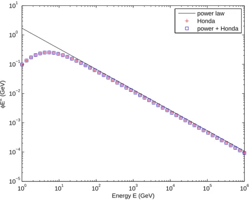
The fitting formula only agree well experiment data below 100 GeV [9] [10]. Table 3.1: Parameters for Eq. (3.1) .

parameter/comp α K b c Hydrogen(A=1) 2.74 14900 2.15 0.21 Iron(A=56) 2.68 4.45 3.07 0.041

But this fitting formula has a power law trend when energy is sufficiently large. Therefore we adopt the power law index -2.7 for energy above 100GeV,

φN(E, 0) =     

k(E + b exp(−c√E))−α _{if E ≤ 10}2_GeV

N0E−2.7 if E > 102GeV.

(3.2) In this work we only consider the contribution of hydrogen (proton).

3.2

Conventional and Prompt Neutrino Flux

For the conventional neutrino flux, kaon decay is the only source of electron neutrino. The electron neutrino is produced through three-body decays

100 101 102 103 104 105 106 10−5 10−4 10−3 10−2 10−1 100 101 Energy E (GeV) φ E 2 (GeV) power law Honda power + Honda

Figure 3.1: Primary flux weighted by E2_{. The solid line for power law, red cross}

K±

→ π0+ e±_{+ ν}

e( ¯νe), KL0 → π±+ e∓+ νe( ¯νe). (3.3)

with branching ratio 4.8% (counting K+ _{and K}− _{separately) and 38.6%}

respec-tively. For conventional differential flux we adopt the formula

φν(E, 0) = BK±_νφ_N(E, 0) (1 − ZN N) ZN K±Z_K±_ν e 1 + βKνcos θE/ǫK± +BKLνφN(E, 0) (1 − ZN N) ZN KLZKLνe 1 + βKνcos θE/ǫKL , (3.4) which is proper for three-body decay. BK±_ν and B_K

Lν are the branching ratio of

K± _{and K}0

L respectively. The parameters of kaon is listed in Table 3.2.

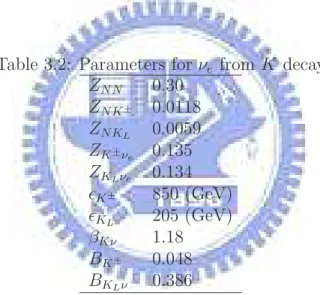
Table 3.2: Parameters for νe from K decay

ZN N 0.30 ZN K± 0.0118 ZN KL 0.0059 ZK±_ν e 0.135 ZKLνe 0.134 ǫK± 850 (GeV) ǫKL 205 (GeV) βKν 1.18 BK± 0.048 BKLν 0.386

The calculation of prompt flux can be divided into three steps: primary cosmic ray, different meson production model and the yield of neutrinos. We then use cascade equations to describe the flux behavior. With the aid of Z moments, source terms of differential flux density have simple forms. For notable critical energy of charm mesons (about 107 _{GeV ), neglecting their interaction in cascade}

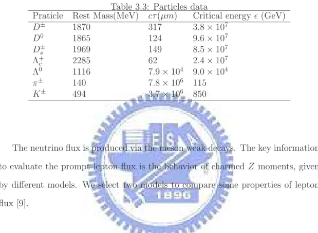
equation is allowable in our interested energy range, TeV to PeV. Then the charm meson flux density is given by low energy limit approximation Eq. (2.21). The critical energy is listed in Table 3.3 taken from [11].

Table 3.3: Particles data

Praticle Rest Mass(MeV) cτ (µm) Critical energy ǫ (GeV) D± _{1870 317 3.8 × 10}7 D0 _{1865 124 9.6 × 10}7 D± s 1969 149 8.5 × 107 Λ+ c 2285 62 2.4 × 107 Λ0 _{1116 7.9 × 10}4 _{9.0 × 10}4 π± ₁₄₀ 7.8 × 106 ₁₁₅ K± ₄₉₄ 3.7 × 106 850

The neutrino flux is produced via the meson weak decays. The key information to evaluate the prompt lepton flux is the behavior of charmed Z moments, given by different models. We select two models to compare some properties of lepton flux [9].

Recombination quark parton model (RQPM) is further divided into two cases according to whether the Feynman-scaling holds or not.

If Feynman scaling holds (RQPM-FS), the charm production Z moments are simply given by

ZN M(γ) = ZN MF S = constants. (3.5)

be energy dependent.

ZN M = ZN MF S (

EN

Eγ

), (3.6)

where ξ = 0.177 − 0.005γ. The relative parameters for FS and SV are shown in Table 3.4. Since Ds has much smaller contribution, we ignore it in the current

calculation. Table 3.4: RQPM ZN M parameters Model γ ξ Eγ Z(D±) Z(D0) Z(Λ+c ) FS 1.62 - - _{4.88 × 10}−4 _{4.73 × 10}−4 _{4.36 × 10}−4 ˜ 1.70 - - _{4.86 × 10}−4 _{4.71 × 10}−4 _{4.34 × 10}−4 ˜ 2.02 - - _{3.14 × 10}−4 _{3.09 × 10}−4 _{2.95 × 10}−4 SV 1.62 0.096 103 _{5.55 × 10}−4 _{5.35 × 10}−4 _{4.9 × 10}−4 ˜ 1.70 0.092 103 _{5.81 × 10}−4 _{5.61 × 10}−4 _{5.2 × 10}−4 ˜ 2.02 0.076 106 _{6.65 × 10}−4 _{6.55 × 10}−4 _{6.2 × 10}−4

The other model is Perturbative QCD(PQCD), as calculated with Monte Carlo by Thunman et al [1]. They use program PYTHIA to generate proton nucleon interaction and the MRSG parton densities. Fig. 3.2 presents curves of Z moments for different charm mesons in logarithmic scale. Curves by meson are carried out by considering whether a primary spectrum has a with knee or not. In this figure, it shows D± _{has less regeneration chance than D}0_{. Charm meson also has lower}

production chance with knee because the primary cosmic ray is steeper above the knee.

The Z moment of Λc and Dscan be obtained by the relation: Z(Λc) ∼ 0.3Z(D)

102 103 104 105 106 107 108 109 E_N (GeV) 0.0000 0.0001 0.0002 0.0003 0.0004 ZN−i ( γ ) D+ − no−knee Do D+ − knee Do pQCD

Figure 3.2: Charm Z-moment for PQCD, considering the primary either with or without a knee, as a function of energy [1].

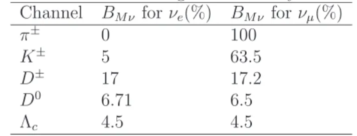
Finally we consider the electron, muon and tau neutrino flux. The prompt neutrinos mainly arise from decays of charm mesons due to the high critical energy of charm. We neglect the interaction channels from the charm meson. Detail decays channel of consideration is in Table 3.5. The charm neutrino differential flux is represented by Eq. (2.23).

Table 3.5: The branching ratio of decays channel. Channel BM ν for νe(%) BM ν for νµ(%)

π± _{0 100}

K± _{5 63.5}

D± _{17 17.2}

D0 _{6.71 6.5}

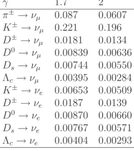
Table 3.6: Decay Z moments for charm and K. γ 1.7 2 π± → νµ 0.087 0.0607 K± → νµ 0.221 0.196 D± → νµ 0.0181 0.0134 D0 → νµ 0.00839 0.00636 Ds→ νµ 0.00744 0.00550 Λc → νµ 0.00395 0.00284 K± → νe 0.00653 0.00509 D± → νe 0.0187 0.0139 D0 → νe 0.00870 0.00660 Ds→ νe 0.00767 0.00571 Λc → νe 0.00404 0.00293

We use decay Z moment ZM ν from Thunman’s work [1] with the Lund Monte

Carlo. The parameters is listed in Table 3.6. The branching ratio of muon neutrinos from charm decays are close to those of electron neutrinos and we consider muon neutrino flux the same as the electron neutrino flux.

The main source of atmospheric τ neutrino is the leptonic decay of the Ds

followed by the τ decay. The calculation for ντ flux is different from those for

νµ and νe because Ds → ντ has more complex mechanism. For two body decay,

Ds decays directly to ντ and its decay Z moment is the same as pion and kaon

decays. But the charge lepton τ from the Ds decay also contributes to the flux of

ντ through chain interaction Ds → τ → ντ. Therefore the actual decay moment

ZDsντ = Z (2 body) Dsντ + Z (chain) Dsντ . (3.7)

3.3

Shower Events

Through weak interactions, neutrinos can be detected by observable showers. The energy Eν of incoming neutrino is shared by hadronic shower, with a faction y

and outgoing lepton with fraction 1 − y. In charge current channel, the resultant charged lepton can be observed. For instance, electrons can easily interact with other substances and produce EM showers. The produced EM shower can not be distinguished from hadronic shower. Therefore we consider both as a single shower event. In charged current process, the energy of electron neutrino totally transfer to the shower energy while in neutral current one hadronic showers get the fraction 1 − y of neutrino energy. In consideration of muon neutrino, because muons can go through a great atmospheric depth, which can travel 6.6 Km at 1 GeV, CC (charged current) shower events can be singled out by muon detectors on the ground. In this work, we exclude CC shower of muon neutrino from all shower events. As for the tau neutrino, the contribution of CC and NC (neutral current) are both included under 107 _{GeV for shower energy. Above 10}7 _{GeV, τ}

lepton can be traced by water cherenkov detector therefore CC interaction of tau neutrino will be separated in high energy.

We adopt Reno’s model as the cross section of CC and NC of neutrino-nucleon interactions which is based on CTEQ4-DIS [2]. The related formula is given by:

           σCC = 5.53 × 10−36(_1GeVEν )0.363cm2 σNC = 2.31 × 10−36(_1GeVEν )0.363cm2 σtotal = 7.84 × 10−36(_1GeVEν )0.363cm2 (3.8)

Eν is incoming neutrino energy in the lab frame. At energy below 104 GeV,

the cross section increases linearly with Eν. The CC cross section is four or five

times greater than NC one.

3.4

Numerical Results on Shower Events Rates

and Angular Dependencies

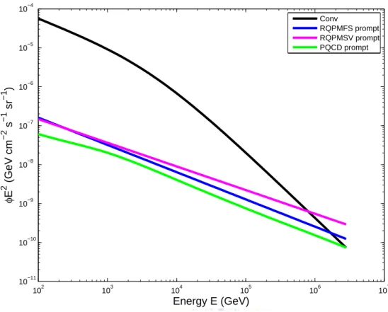
First we compare different prompt flux results in Figure 3.4 and Figure 3.5 with the conventional one along vertical and horizontal directions. The intersection of conventional and prompt fluxes locate around 105_{GeV which is consistent with the}

result of Beacom et al [14]. However, in the horizontal direction, the intersection lies around 106 _{GeV due to the fact that the conventional flux is enhanced in the}

large zenith angle.

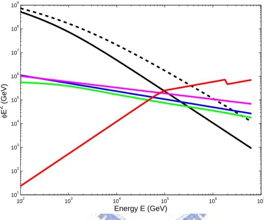
For shower events, we use a 1km3 _{cubic volume of water as shower}

de-tector and take three years of data. Figure 3.6 is showers flux spectra in lower zenith angle for three years of data-taking. The discontinuity in GRB is due to that leptons from CC of τ neutrino can be distinguishable above 106_GeV.

Figure 3.3: Cross section for νN interactions at high energies according to CTEQ4-DIS parton distribution [2].

102 103 104 105 106 107 10−12 10−11 10−10 10−9 10−8 10−7 10−6 10−5 10−4 Energy E (GeV) φ E 2 (GeV cm −2 s −1 sr −1 ) Conv RQPMFS prompt RQPMSV prompt PQCD prompt

Figure 3.4: The comparison of electron neutrino fluxes given by different models. The y-axis is the weighted flux spectra and x-axis is the neutrino energy in GeV unit. This is for the zenith angle 0◦_.

102 103 104 105 106 107 10−11 10−10 10−9 10−8 10−7 10−6 10−5 10−4 Energy E (GeV) φ E 2 (GeV cm −2 s −1 sr −1 ) Conv RQPMFS prompt RQPMSV prompt PQCD prompt

Figure 3.5: This shows the electron neutrino flux in the horizontal direction. The intersection of conventional and prompt fluxes locates around 106 _{GeV due to the}

102 103 104 105 106 107 101 102 103 104 105 106 107 108 109 Energy E (GeV) φ E 2 (GeV)

Figure 3.6: Event number spectra for three years of data-taking in km3 _water

Cherenkov detector. The black lines are conventional shower events. The solid one is shower events from the low zenith angle bin θ = [0◦_{, 60}◦_{]. The dashed one}

is shower events from the high zenith angle bin θ = [60◦_{, 90}◦_{]. The colored lines}

are prompt and GRB(red) shower events. The prompt and GRB shower event are isotropic. The magenta line means RQPM-SV model for shower events. The blue and green lines represent the RQPM-FS and PQCD models for shower events respectively.

We suggest a method to probe the footprint of prompt flux. The diffuse source and prompt flux are isotropic and the conventional flux has an angular dependence. Then we divide the data into two bins, high zenith angle and low zenith angle bins. The low bins covers the range of zenith angle from 0◦ _{to 60}◦_;

the rest is the high bin. We define ratio R which is the shower event rate at the low bin divided by that at the high bin:

R = small zenith angle events

large zenith angle events. (3.9) In each energy bin, we also vary the shower energy threshold, which is denoted by Ec.

Figure 3.7 is the shower events ratio R verse the threshold energy Ec. At the

low energy, the flux is dominated by the conventional component resulting from the decays of pions and kaons. However the prompt flux overtakes the conventional component in the PeV energy range. We present the result for integrated flux where Ec is the lower limit of the integration. The flux ratio is smaller in the

horizontal direction since the conventional flux is enhanced in this case.

There are characteristic in these ratios. The ratio of conventional flux shows a plateau at the high energy. In Eq. (3.4), the ratio of conventional differential flux has the limit as the neutrino energy is large enough. This causes that the ratio between the integrated shower event rate in low and high bin reaches the above limit value. The second is the trend of the ratio in high energy. This is because prompt flux is isotropic and at the high energy the prompt flux is dominant over the conventional flux. With GRB flux added the ratio rises early since GRB flux is even more dominant in high energy. The addition of GRB flux makes model

102 103 104 105 106 107 0 0.1 0.2 0.3 0.4 0.5 0.6 0.7 0.8 0.9 1 Cut Energy E c (GeV) Ratio

Figure 3.7: Ratio versus energy threshold Ec. The black curve represents the ratio

for the conventional flux. The flux ratio including contributions of the prompt flux is represented by the dotted color line. According to different charm production models used to calculate the prompt flux, the magenta, blue and green dotted lines represent total flux ratios where the prompt component of the flux is calculated by RQPM-SV, RQPM-FS ans PQCD models respectively. The solid color lines denote flux ratios with the GRB neutrino flux also added into the total flux.

dependencies in the prompt flux diminish. In this case, it is more difficult to distinguish models for the prompt flux. However the presence of GRB flux makes the neutrino astronomy exciting.

Chapter 4

Conclusion

• We have proposed to identify conventional and prompt atmospheric neu-trino flux as well as neuneu-trinos flux from the extragalctic sources through the angular dependencies of shower events.

• We have shown the prompt flux overtakes the conventional component in the PeV energy range.

• The ratio of shower event decreases monotonically for conventional atmo-spheric neutrinos as we raise the shower energy threshold.

• Both the prompt atmospheric neutrino flux and the neutrinos from extra-galactic diffusive sources are isotropic. Their presence raises the above-mentioned ratio.

• GRB flux dominates that of prompt atmospheric neutrinos in our interested energy range. The presence of GRB flux will obliterate the footprint of prompt fluxes.

In the following tables, we use the duple with conventional shower event rate as the first number and prompt event rate that as the second number.

Table 4.1: Ec = 1.0 × 105 GeV, 10 years of data taking. R=0.12 for conventional

ν’s

Model PQCD RQPM RQPM-FS small (3.3,1.9) (3.3,5.0) (3.3,2.7) large (26.6,1.9) (26.6,5.0) (26.6,2.7)

R 0.18 0.26 0.20

Table 4.2: Ec = 2.5 × 105 GeV, 10 years of data taking. R=0.11 for conventional

ν’s

Model PQCD RQPM RQPM-FS small (0.38,0.55) (0.38,1.6) (0.38,0.78) large (3.6,0.55) (3.6,1.6) (3.6,0.78)

R 0.23 0.38 0.26

Table 4.3: Ec = 5.0 × 105 GeV, 10 years of data taking. R=0.10 for conventional

ν’s

Model PQCD RQPM RQPM-FS small (0.077,0.22) (0.077,0.66) (0.077,0.31) large (0.79,0.22) (0.79,0.66) (0.79,0.31)

R 0.29 0.51 0.35

Table 4.4: Ec = 1.0 × 105 GeV, 10 years of data taking. R=0.13 for conventional ν’s Model PQCD RQPM RQPM-FS GRB only small (3.3,1.9) (3.3,5.0) (3.3,2.7) 12 large (26.6,1.9) (26.6,5.0) (26.6,2.7) 12 R 0.18 0.26 0.20 -RGRB 0.42 0.47 0.44

-Table 4.5: Ec = 2.5 × 105 GeV, 10 years of data taking. R=0.11 for conventional

ν’s Model PQCD RQPM RQPM-FS GRB only small (0.38,0.55) (0.38,1.6) (0.38,0.78) 6.1 large (3.6,0.55) (3.6,1.6) (3.6,0.78) 6.1 R 0.23 0.38 0.26 -RGRB 0.69 0.72 0.70

-Table 4.6: Ec = 5.0 × 105 GeV, 10 years of data taking. R=0.10 for conventional

ν’s Model PQCD RQPM RQPM-FS GRB only small (0.077,0.22) (0.077,0.66) (0.077,0.31) 3.5 large (0.79,0.22) (0.79,0.66) (0.79,0.31) 3.5 R 0.29 0.51 0.35 -RGRB 0.84 0.86 0.84

-Bibliography

[1] M. Thunman, G. Ingelman, and P. Gondolo, “Charm production and high energy atmospheric muon and neutrino fluxes,” Astroparticle Physics, vol. 5, p. 309, 1996.

[2] R. Gandhi, C. Quigg, M. H. Reno, and I. Sarcevic, “Neutrino interactions at ultrahigh energies,” Physical Review D, vol. 58, p. 093009, 1998.

[3] F. Halzen, “Lectures on high-energy neutrino astronomy,” 2005.

[4] L. Bergstrom and A. Goobar, Cosmology and Particle Astrophysics. Springer . Press, 2004.

[5] J. N. Bahcall and E. Waxman, “Has the gzk suppression been discovered?,” Physics Letters B, vol. 556, no. 1-2, pp. 1–6, 2003/3/13.

[6] P. Lipari, “Lepton spectra in the earth’s atmosphere,” Astroparticle Physics, vol. 1, no. 2, pp. 195–227, 1993/3.

[8] F.-F. Lee and G.-L. Lin, “A semi-analytic calculation on the atmospheric tau neutrino flux in the gev to tev energy range,” Astroparticle Physics, vol. 25, pp. 64–73, 2 2006.

[9] T. K. Gaisser and M. Honda, “Flux of atmospheric neutrinos,” Annual Review of Nuclear and Particle Science, vol. 52, p. 153, 2002.

[10] M. Honda, T. Kajita, K. Kasahara, and S. Midorikawa, “Calculation of the flux of atmospheric neutrinos,” Phys.Rev.D, vol. 52, pp. 4985–5005, Nov 1995. [11] C. G. S. Costa, “The prompt lepton cookbook,” Astroparticle Physics, vol. 16,

pp. 193–204, November, 2001 2001.

[12] L. Pasquali, M. H. Reno, and I. Sarcevic, “Lepton fluxes from atmospheric charm,” Phys.Rev.D, vol. 59, p. 034020, Jan 1999.

[13] L. Pasquali and M. H. Reno, “Tau neutrino fluxes from atmospheric charm,” Physical Review D, vol. 59, p. 093003, 03/23/ 1999. ID: 10.1103/Phys-RevD.59.093003; J1: PRD.

[14] J. F. Beacom and J. Candia, “Shower power: Isolating the prompt atmo-spheric neutrino flux using electron neutrinos,” JCAP, vol. 0411, p. 009, 2004.