以休息狀態腦磁波進行情感性疾病之分類

全文

(1)國立交通大學多媒體工程研究所碩士論文. 以休息狀態腦磁波進行情感性疾病之分類 Classification of Mood Disorders from Resting MEG Signals. 研究生：黃詠恬指導教授：陳永昇. 中華民國. 博士. 九十七. 年九月.

(2) 2.

(3) 以休息狀態腦磁波進行情感性疾病之分類 Classification of Mood Disorders from Resting MEG Signals. 研究生：黃詠恬. Student：Yung-Tien Huang. 指導教授：陳永昇. Advisor：Yong-Sheng Chen. 國立交通大學多媒體工程研究所碩士論文. A Thesis Submitted to Institute of Multimedia Engineering College of Computer Science National Chiao Tung University in partial Fulfillment of the Requirements for the Degree of Master in. Computer Science September 2008 Hsinchu, Taiwan, Republic of China. 中華民國九十七年九月.

(4) 4.

(5) 摘. 要. 近年來，受情感性疾病 (Mood Disorder) 所苦的病患日益增加，此類疾患嚴重擾亂病人的情緒，進而對日常生活層面造成不良影響，而其中又屬躁鬱症 (Bipolar Disorder) 以及重鬱症 (Major Depressive Disorder) 最廣為所知。情緒性疾病已漸漸成為現代人的主要疾病之一，關於此類疾病的各方面研究也在近數十年內蓬勃發展，其中，患者腦部結構與功能的異常被認為是情感性疾病的重要病因之一。關於情感性疾病在腦部異常的研究，主要分為腦結構影像與腦波訊號兩方面。然而現今對於患者腦波的研究仍顯不足，最主要的困難之一在於如何自腦波訊號中擷取具有鑑別力的訊號特徵。在本篇論文當中，我們和台北榮民總醫院合作，取得情緒性疾病患者在休息狀態的腦磁波 (Magnetoencephalography) 訊號量測資料。受試者包含二十六位躁鬱症患者、二十二位重鬱症患者以及二十五位做為對照組的健康受試者。在本篇研究中我們分析研究這三個群組的腦磁波訊號，提出具有鑑別力的訊號特徵並且對此三群組加以分類。在本篇論文中我們使用三種類型的特徵擷取方法，其一是從功率頻譜密度 (Power Spectrum Density)中所擷取的特徵，其次為時序訊號上的複雜度，包含 Lempel-Ziv Complexity 以及 Sample Entropy，最後再總合前兩類型特徵以取得左右半腦非對稱性的特徵。針對所擷取的特徵，我們使用統計學中的 T 檢定 (t-test)以及線性判別分析(Linear Discriminant Analysis)的方法，挑出有鑑別力的訊號特徵並藉以將特徵空間的維度降至合理的範圍。在本篇論文中我們對所擷取的特徵做了詳細的分析與探討，此外並使用支援向量機(Support Vector Machine)作為分類器。最後，在任兩群組以及三個群組的分類中得到良好的分類正確率，證明用於本篇論文中的訊號特徵對於情感性疾病具有一定程度的鑑別能力。.

(6) 6.

(7) 誌. 謝. 感謝陳永昇與陳麗芬老師，除了在學術上的成就，也在為人處事上豎立典範，兩年間不只有學業上的指導，更有生活上的鼓勵與關心。也要感謝我的父母二十多年來對我的養育與栽培、兄長朋友的關心以及男朋友的鼓勵，一切都是因為有你們的支持。.

(8) 8.

(9) Classification of Mood Disorders from Resting MEG Signals. A thesis presented by. Yung-Tien Huang to. Institute of Multimedia Engineering College of Computer Science in partial fulfillment of the requirements for the degree of Master in the subject of. Computer Science National Chiao Tung University Hsinchu, Taiwan 2008.

(10) Classification of Mood Disorders from Resting MEG Signals. c 2008 Copyright by Yung-Tien Huang.

(11) Abstract. Recently, more and more people are suffering from mood disorders such as Bipolar Disorder(BD) and Major Depressive Disorder(MDD). These mood disorders have become one of the major illness of modern people. Therefore, researchers are attempting to study these disorders in different areas, including the abnormality of brain structure and brain signals. However, studies about the abnormality of brain signals are still insufficient and inconsistent. One of the main difficulties is to obtain significant features for further analysis. In this work, we studied three groups of resting Magnetoencephalographic signal data collected by Taipei Veterans General Hospital, including 26 patients with BD, 22 patients with MDD, and 25 normal controls. We then proposed a procedure to classify the three study groups from each others. In this work, we studied features obtained from power spectrum density, Lempel-Ziv complexity, sample entropy, multi-scale entropy, and hemispheric asymmetry. After the feature extraction, t-test and Linear Discriminant Analysis were applied as feature selection and also to reduce the features to a reasonable number. We provided methodical analysis of the selected features. Furthermore, we applied Support Vector Machine to classify the three groups. The results showed an almost 100% accuracy in the classification, verifying the significance of our features.. i.

(12) ii.

(13) Contents List of Figures. v. List of Tables. vii. 1. 2. 3. Introduction 1.1 Mood Disorders . . . . . . . . . . . . . . . . . . . . . . . . . 1.1.1 Bipolar Disorder . . . . . . . . . . . . . . . . . . . . 1.1.2 Major Depressive Disorder . . . . . . . . . . . . . . . 1.2 Relative Researches . . . . . . . . . . . . . . . . . . . . . . . 1.2.1 Structural Abnormalities of Mood Disorder Patients . 1.2.2 Brain Signal Abnormalities of Mood Disorder Patients 1.2.3 Hemispheric Asymmetry . . . . . . . . . . . . . . . . 1.3 Magnetoencephalographic studies of mood disorders . . . . . 1.4 Thesis Scope . . . . . . . . . . . . . . . . . . . . . . . . . . Feature Extraction 2.1 ROI . . . . . . . . . . . . . . . 2.2 PSD features . . . . . . . . . . 2.2.1 Band Powers . . . . . . 2.2.2 Spectral Measures . . . 2.2.3 Spectral Ratio Measures 2.2.4 Spectral Entropy . . . . 2.3 Temporal Complexity . . . . . . 2.3.1 Lempel-Ziv Complexity 2.3.2 Sample Entropy . . . . . 2.3.3 Multi-Scale Entropy . . 2.4 Hemispheric Asymmetry . . . .. . . . . . . . . . . .. . . . . . . . . . . .. . . . . . . . . . . .. . . . . . . . . . . .. . . . . . . . . . . .. . . . . . . . . . . .. . . . . . . . . . . .. . . . . . . . . . . .. . . . . . . . . . . .. . . . . . . . . . . .. . . . . . . . . . . .. . . . . . . . . . . .. . . . . . . . . . . .. . . . . . . . . . . .. . . . . . . . . . . .. . . . . . . . . . . .. . . . . . . . . .. . . . . . . . . . . .. . . . . . . . . .. . . . . . . . . . . .. . . . . . . . . .. . . . . . . . . . . .. . . . . . . . . .. . . . . . . . . . . .. . . . . . . . . .. . . . . . . . . . . .. . . . . . . . . .. . . . . . . . . . . .. . . . . . . . . .. 1 2 2 3 4 4 6 6 7 8. . . . . . . . . . . .. 9 10 10 10 11 12 14 15 15 17 18 20. Classification 23 3.1 Linear Discriminant Analysis . . . . . . . . . . . . . . . . . . . . . . . . . 25 3.1.1 Introduction to LDA . . . . . . . . . . . . . . . . . . . . . . . . . 25 iii.

(14) 3.2 4. 5. 6. 3.1.2 Feature Selection . . . . . . . . . . . . . . . . . . . . . . . . . . . 26 Support Vector Machine . . . . . . . . . . . . . . . . . . . . . . . . . . . 28. Experiment Results 4.1 Materials . . . . . . . . . . . . . . . . . . . . . . . . . 4.1.1 Subjects . . . . . . . . . . . . . . . . . . . . . . 4.1.2 MEG Device . . . . . . . . . . . . . . . . . . . 4.1.3 MEG Data Collection . . . . . . . . . . . . . . 4.2 Data Preprocessing . . . . . . . . . . . . . . . . . . . . 4.3 Features of Power Spectrum . . . . . . . . . . . . . . . 4.3.1 band power . . . . . . . . . . . . . . . . . . . . 4.3.2 MF and SEF90 . . . . . . . . . . . . . . . . . . 4.3.3 Spectral Ratio Measures . . . . . . . . . . . . . 4.3.4 Spectral Entropy . . . . . . . . . . . . . . . . . 4.4 Temporal Complexity . . . . . . . . . . . . . . . . . . . 4.4.1 LZC . . . . . . . . . . . . . . . . . . . . . . . . 4.4.2 SampEn . . . . . . . . . . . . . . . . . . . . . . 4.5 Hemispheric Asymmetry . . . . . . . . . . . . . . . . . 4.5.1 Band Power . . . . . . . . . . . . . . . . . . . . 4.5.2 Spectral Measures . . . . . . . . . . . . . . . . 4.5.3 Spectral Ratio Measures . . . . . . . . . . . . . 4.5.4 Spectral Entropy . . . . . . . . . . . . . . . . . 4.5.5 Lempel-Ziv Complexity . . . . . . . . . . . . . 4.5.6 Sample Entropy . . . . . . . . . . . . . . . . . . 4.6 Classification Results . . . . . . . . . . . . . . . . . . . 4.6.1 Normal Control vs. Bipolar Disorder . . . . . . 4.6.2 Normal Control vs. Major Depressive Disorder . 4.6.3 Bipolar Disorder vs. Major Depressive Disorder 4.6.4 The three groups classificaiton . . . . . . . . . . 4.7 Correlation Between Rating and Features . . . . . . . . Discussion 5.1 Suitable Spectral Ratios for Mood Disorders . . 5.2 Spectral Entropies . . . . . . . . . . . . . . . . 5.3 The Parameters in Multi-scale Sample Entropy 5.4 Features for Classification . . . . . . . . . . . Conclusions. . . . .. . . . .. . . . .. . . . .. . . . .. . . . . . . . . . . . . . . . . . . . . . . . . . .. . . . .. . . . . . . . . . . . . . . . . . . . . . . . . . .. . . . .. . . . . . . . . . . . . . . . . . . . . . . . . . .. . . . .. . . . . . . . . . . . . . . . . . . . . . . . . . .. . . . .. . . . . . . . . . . . . . . . . . . . . . . . . . .. . . . .. . . . . . . . . . . . . . . . . . . . . . . . . . .. . . . .. . . . . . . . . . . . . . . . . . . . . . . . . . .. . . . .. . . . . . . . . . . . . . . . . . . . . . . . . . .. . . . .. . . . . . . . . . . . . . . . . . . . . . . . . . .. . . . .. . . . . . . . . . . . . . . . . . . . . . . . . . .. 33 34 34 34 36 36 37 37 41 43 46 47 47 52 57 57 59 61 65 65 69 73 73 75 78 80 83. . . . .. 91 92 92 94 97 99. Bibliography. 103. iv.

(15) List of Figures 1.1. Framework . . . . . . . . . . . . . . . . . . . . . . . . . . . . . . . . . .. 2.1 2.2 2.3 2.4 2.5. Schematic illustration of the MEG sensor layout and the ROIs. . . . . . . Schematic representation of MF and SEF90. . . . . . . . . . . . . . . . . LZC concept. . . . . . . . . . . . . . . . . . . . . . . . . . . . . . . . . the concept of sample entropy. . . . . . . . . . . . . . . . . . . . . . . . Schematic illustration of the MEG sensor layout and the ROIs for asymmetric analysis. . . . . . . . . . . . . . . . . . . . . . . . . . . . . . . .. . . . .. 3.1 3.2 3.3 3.4 3.5. Classification procedures. . . . . . . . . . . . . . . . An idea of LDA projection. . . . . . . . . . . . . . . The weighting of LDA projection matrix. . . . . . . The idea of selecting separating hyperplain in SVM. . Margin and support vectors of SVM. . . . . . . . . .. . . . . .. . . . . .. . . . . .. . . . . .. . . . . .. . . . . .. . . . . .. . . . . .. . . . . .. . . . . .. . . . . .. . . . . .. 24 25 27 28 29. 4.1 4.2 4.3 4.4 4.5 4.6 4.7 4.8 4.9 4.10 4.11 4.12 4.13 4.14 4.15 4.16. MEG device . . . . . . . . . . . . . . . . . . . Preprocessing procedures for MEG recordings . Relative band power . . . . . . . . . . . . . . MF and SEF90 . . . . . . . . . . . . . . . . . Spectral Ratios. . . . . . . . . . . . . . . . . . Spectral Entropies. . . . . . . . . . . . . . . . Multi-scale LZC. . . . . . . . . . . . . . . . . Multi-scale entorpy (SampEn). . . . . . . . . . Hemispheric asymmetry of relative band power. Hemispheric asymmetry of MF and SEF90. . . Hemispheric asymmetry of spectral ratios. . . . Hemispheric asymmetry of spectral entropies. . Results of the NC and BD classification. . . . . Results of the NC and MDD classification. . . . Results of the BD and MDD classification. . . . Results of the 3-groups classification. . . . . .. . . . . . . . . . . . . . . . .. . . . . . . . . . . . . . . . .. . . . . . . . . . . . . . . . .. . . . . . . . . . . . . . . . .. . . . . . . . . . . . . . . . .. . . . . . . . . . . . . . . . .. . . . . . . . . . . . . . . . .. . . . . . . . . . . . . . . . .. . . . . . . . . . . . . . . . .. . . . . . . . . . . . . . . . .. . . . . . . . . . . . . . . . .. . . . . . . . . . . . . . . . .. 35 37 38 41 44 46 48 53 58 60 63 64 75 75 78 80. v. . . . . . . . . . . . . . . . .. . . . . . . . . . . . . . . . .. . . . . . . . . . . . . . . . .. 8 11 12 17 19. . 21.

(16) 5.1 5.2. The influence of different r in multi-scale sample entropy. . . . . . . . . . 95 The influence of different m in multi-scale sample entropy. . . . . . . . . . 96. vi.

(17) List of Tables 1.1. Brain structural changes reported in mood disorders. . . . . . . . . . . . .. 4.1 4.2 4.3 4.4 4.5 4.6 4.7 4.8 4.9 4.10 4.11 4.12. Demographic data of subjects. . . . . . . . . . . . . . . . . . . . . . . . The p-values of band power between NC and BD. . . . . . . . . . . . . . The p-values of band power between NC and MDD. . . . . . . . . . . . . The p-values of band power between BD and MDD. . . . . . . . . . . . . The p-values of mean frequency (MF). . . . . . . . . . . . . . . . . . . . The p-values of the 90% spectral edge frequency (SEF90) . . . . . . . . . The p-values of spectral ratios between NC and BD. . . . . . . . . . . . . The p-values of spectral ratios between NC and MDD. . . . . . . . . . . The p-values of spectral ratios between BD and MDD. . . . . . . . . . . The p-values of spectral antropy 1 (SE1). . . . . . . . . . . . . . . . . . The p-values of spectral antropy 2 (SE2). . . . . . . . . . . . . . . . . . The p-values of Lempel-Ziv complexity (LZC) between NC and BD in multiple scales. . . . . . . . . . . . . . . . . . . . . . . . . . . . . . . . The p-values of Lempel-Ziv complexity (LZC) between NC and MDD in multiple scales. . . . . . . . . . . . . . . . . . . . . . . . . . . . . . . . The p-values of Lempel-Ziv complexity (LZC) between BD and MDD in multiple scales. . . . . . . . . . . . . . . . . . . . . . . . . . . . . . . . The p-values of sample entropy (SampEn) between NC and BD in multiple scales. . . . . . . . . . . . . . . . . . . . . . . . . . . . . . . . . . . . . The p-values of sample entropy (SampEn) between NC and MDD in multiple scales. . . . . . . . . . . . . . . . . . . . . . . . . . . . . . . . . . The p-values of sample entropy (SampEn) between BD and MDD in multiple scales. . . . . . . . . . . . . . . . . . . . . . . . . . . . . . . . . . The p-values of band power asymmetry between NC and BD. . . . . . . . The p-values of band power asymmetry between NC and MDD. . . . . . The p-values of band power asymmetry between BD and MDD. . . . . . The p-values of MF asymmetry. . . . . . . . . . . . . . . . . . . . . . . The p-values of SEF90 asymmetry. . . . . . . . . . . . . . . . . . . . . . The p-values of spectral ratio asymmetry between NC and BD. . . . . . .. 4.13 4.14 4.15 4.16 4.17 4.18 4.19 4.20 4.21 4.22 4.23. vii. . . . . . . . . . . .. 5 35 39 39 40 42 42 43 45 45 46 47. . 49 . 50 . 51 . 54 . 55 . . . . . . .. 56 57 59 59 60 60 61.

(18) 4.24 4.25 4.26 4.27 4.28 4.29 4.30 4.31 4.32 4.33 4.34 4.35 4.36 4.37 4.38 4.39 4.40 4.41 4.42 4.43 4.44 4.45 4.46 4.47 5.1. The p-values of spectral ratio asymmetry between NC and MDD. . . . . . . The p-values of spectral ratio asymmetry between BD and MDD. . . . . . . The p-values of spectral entropy 1 (SE1) asymmetry. . . . . . . . . . . . . The p-values of spectral entropy 2 (SE2) asymmetry. . . . . . . . . . . . . The p-values of LZC asymmetry between NC and BD in multiple scales. . . The p-values of LZC asymmetry between NC and MDD in multiple scales. The p-values of LZC asymmetry between BD and MDD in multiple scales. The p-values of SampEn asymmetry between NC and BD in multiple scales. The p-values of SampEn asymmetry between NC and MDD in multiple scales. . . . . . . . . . . . . . . . . . . . . . . . . . . . . . . . . . . . . . The p-values of SampEn asymmetry between BD and MDD in multiple scales. . . . . . . . . . . . . . . . . . . . . . . . . . . . . . . . . . . . . . The features used in NC and BD classification. . . . . . . . . . . . . . . . The features used in NC and MDD classification. . . . . . . . . . . . . . . The features used in NC and MDD classification. . . . . . . . . . . . . . . The confusion matrix of the BD and MDD classification. . . . . . . . . . . The features used in BD and MDD classification. . . . . . . . . . . . . . . The features used in 3-groups classification. . . . . . . . . . . . . . . . . . The features used in 3-groups classification. . . . . . . . . . . . . . . . . . Demographic data of subjects. . . . . . . . . . . . . . . . . . . . . . . . . The significance of correlation between ratings and features in the BD case. The significance of correlation between ratings and features in the BD case. The significance of correlation between ratings and features in the MDD case. . . . . . . . . . . . . . . . . . . . . . . . . . . . . . . . . . . . . . . The significance of correlation between ratings and features in the MDD case. . . . . . . . . . . . . . . . . . . . . . . . . . . . . . . . . . . . . . . The significance of correlation between ratings and features in the MDD case. . . . . . . . . . . . . . . . . . . . . . . . . . . . . . . . . . . . . . . The significance of correlation between ratings and features in the MDD case. . . . . . . . . . . . . . . . . . . . . . . . . . . . . . . . . . . . . . .. 62 62 64 64 66 67 68 70 71 72 74 76 77 78 79 81 82 83 84 85 86 87 88 89. Comparison of different spectral ratios. . . . . . . . . . . . . . . . . . . . 93. viii.

(19) Chapter 1 Introduction.

(20) 2. Introduction. The first chapter is a brief introduction about some background knowledge of this thesis. Nowadays mood disorders have been common diseases which effect daily life ill. We first briefly introduce the mood disorders in section 1.1 and then focus on bipolar disorder and major depressive disorder. Both bipolar disorder and major depressive disorder are reported intently relating to brain abnormalities, and are described in the section 1.2.. 1.1. Mood Disorders. Nowadays many people suffer from mood disorders. Mood disorders, also known as affective disorders, are a grouping of psychiatric diseases where the primary symptom is a disturbance in mood. The patients with mood disorders not only suffer from the abnormalities of mood, but also the differences of biological, behavioral, and social aspects. According to DSM-IV (Diagnostic and Statistical Manual of Mental Disorders 4th Edition), which was published by the American Psychiatric Association in 1994, four disorders are included in the category of mood disorders: bipolar disorder, cyclothymic disorder, dysthymic disorder and major depressive disorder. Bipolar disorder and major depressive disorder are the most well-known disorders among them, and what follows is a brief introduction of the two disorders.. 1.1.1. Bipolar Disorder. Bipolar disorder (BD), also known as manic-depressive disorder and bipolar affective mood disorder, is a kind of mood disorder that causes unusual shifts in a person’s mood. And the influences of BD also extend many aspects like sleep, energy, and ability to function. People with bipolar disorder periodically exhibit mood episodes including depressive episodes, manic episodes and mixed episodes. During depressive episodes, individuals usually experience low mood, feel sad, diminished interest in usual activities and disturbances in sleep, appetite, energy, and concentration. Manic episodes typically involve either extremely happy or irritable mood, accompanied by other changes in behavior, such as increased activity, decreased need for sleep, flight of ideas, and racing thoughts. Mixed.

(21) 1.1 Mood Disorders. episodes include the features of both mania and depression episodes presented at the same time. The duration of mood episodes typically lasts from a couple of hours to many months. Between episodes people with BD often return to their usual functioning and personality. There are two diagnostic types in bipolar disorder according to the type and severity of mood episodes experienced. Bipolar I disorder is characterized by severe mania episodes and depression. For a diagnosis of bipolar I disorder, a person must have at least one manic episode. Bipolar II disorder is characterized by hypomania episodes and often followed by periods of severe depression. Up to now, the clinical causes of bipolar disorder are still unknown. Studies suggest that there may be many contributory factors acting together to produce the illness, such as genetics, stress, environmental factors, neurobiology, and psychological and social processes. In recent decades, many studies have attempted to clarify the neural substrates of bipolar disorder, and inferred that bipolar disorder has been associated with abnormalities of brain structure and function.. 1.1.2. Major Depressive Disorder. Major depressive disorder (MDD) is also known as major depression, unipolar depression, or clinical depression. This may be compared with bipolar depression which has the two poles of depressed mood and mania (i.e., euphoria, heightened emotion and activity). It is a kind of mood disorders which is characterized by a pervasive and recurrent low mood or loss of interest or pleasure in usual activities. Different from patients of bipolar disorder, patients with major depressive disorder experience at least one major depressive episodes but without manic episodes. A major depressive episode has been defined as a severely depressed mood that persists for at least two weeks. The patients suffer from recurrent depressive moods, and may feel sad, worthless, guilty or empty, lose energy and interests in daily life. Some of them also suffer from sleep disturbances (sleeplessness or too much sleeping). There are also difficulties in concentrating, social life, and even working. For some, the pain from MDD effects life so deeply that MDD becomes a major risk factor of suicide. Causes of major depressive disorder can be roughly classified into two categories, the. 3.

(22) 4. Introduction. psychological and the biological. In the psychological aspect, the causes may be stress, environment or life experiences. In the biological aspect, researches have shown that depression is influenced by genetic and brain abnormalities.. 1.2. Relative Researches. Although mood disorders affect daily life so significant and have become common diseases nowadays, the specific cause of these disorders are still a mystery. In recent years, scientists and clinicians have reached general agreement that these disorders are strongly correlated with brain dysfunction. The researches about brain abnormalities can be roughly divided to two categories, brain structural changes and brain signal abnormalities.. 1.2.1. Structural Abnormalities of Mood Disorder Patients. In the past decades, the development of neuroimaging techniques has produced a proliferation of studies that have attempted to clarify the brain abnormalities responsible for mood disorders. The modalities such as positron emission tomography (PET), computed X-ray tomography (CT), and particularly magnetic resonance imaging (MRI) have contributed to found the structural abnormalities in mood disorders undoubtedly. And Table 1.2.1 summarizes the studies which reported structural changes in bipolar disorder and major depressive disorder [36, 37, 39, 40]. In the BD case, some apparent abnormalities were found. Researchers examined whole brain volumes and found that although the overall brain volumes of BD patients do not different from volumes of healthy controls, but a global decrease in cortical gray matter was conclusive, especially in prefrontal cortex (PFC). The temporal cortex was also reported to be abnormal for many times, but the volume changes are not consistent in these researches. In the subcortical level, abnormalities of enlargements were reported in amygdala, thalamus, and striatum including caudate nucleus and putamen. Besides cortical and subcortical findings, enlargements of ventricles were found, and be obvious in lateral ventricle and the third ventricle. Moreover, abnormal reduction was found in cerebellar vermis, which is generally thought to modulate movement..

(23) N. N. N. Putamen. Thalamus. N. N. N. H. Caudate Nucleus. striatum. Basal Ganglia. Hippocampus. Amygdala. Limbic System ∗. ∗. Temporal Lob. Subcortical. ∗. PFC. Cortical. ∗. ∗. N. N. Lateral Ventricular. Sheline [36]. N N. H. Strakowski [40]. N. H. Strakowski [39]. Bipolar Disorder. 3rd Ventricular. Ventricular. Cerebellar vermis. Cerebellum. Research. ∗. N. ∗. N. N. H. Soares [37]. H. H. H. H. H. H. H. H. ∗. H. Sheline [36]. ∗. H. N. N. H. Strakowski [39]. H. H. H. H. H. N. H. Soares [37]. Major Depressive Disorder. Table 1.1: Brain structural changes reported in mood disorders. The table summarizes some reviews of neuroimaging studies reporting structural abnormalities of mood disorders. The black triangle N represents the increase of volumn size, and black inverted triangle H stands for decrease of volumn size on the contrary. Besides, some structures have been widely reported to different from healthy subjects, but there were no consistant opinions on enlargement or atrophy. We represent these changes as ∗.. 1.2 Relative Researches 5.

(24) 6. Introduction. In the MDD case, prefrontal cortex atrophy, cerebellar vermis atrophy and ventricular enlargements were also found. Contrast to BD patients, the subcortical abnormalities of MDD patients are decreasing volumes of basal ganglia and hippocampus. The structural change of amygdala was also discussed, but there is no conclusion about atrophy or enlargement.. 1.2.2. Brain Signal Abnormalities of Mood Disorder Patients. Conpare with neuroimaging, the number of studies relative to brain signal abnormalities about mood disorder is small, and the study results disagree with each others, especially in the BD case. In the MDD case, most researches in resting brain signals are with EEG. These researches indicated that MDD patients had decreased relative delta band power and increased relative theta and alpha band powers [16, 34]. Some indicated increased relative beta band power [16, 26], but some indicated decreased power [34]. Besides band powers, coherence was also reported to decrease [26, 34], the correlation of left temporocentral is related to the severity of depression, and the theta band correlation disappears in MDD patients [28].. 1.2.3. Hemispheric Asymmetry. Hemispheric asymmetry is the relative imbalance of cerebral activities. Resting frontal EEG asymmetry in the alpha frequency band is believed to reflect certain emotions and behaviors. It has been proposed that individuals with greater left than right frontal brain activity are more likely to have the behaviors with approach motivation and positive affect, while individuals with greater right versus left frontal brain activity are more likely to behave with withdrawal and negative affect [45]. Besides, Graae found an abnormality of EEG asymmetry in female adolescent suicide attempters, and suicidal adolescents had a greater alpha power over left than right hemisphere [20]. Many studies tried to found out the relationship between asymmetry and mood disorders. Asymmetrical resting frontal EEG not only distinguishes currently depressed individuals from nondepressed individuals, but also distinguishes previously depressed eu-.

(25) 1.3 Magnetoencephalographic studies of mood disorders. thymic individuals from individuals without a history of depression [22]. Some indicated that frontal EEG asymmetry is sensitive to mood disorder in adults and may characterize adolescents at risk for mood disorder [43]. Some studies measuring EEG asymmetry in depressed subjects found the greater left than right alpha band power [9] and reduced left hemisphere activation [26]. In the BD case, it was reported that increased relative right frontal activity has been observed in bipolar depression, whereas increased relative left frontal activity has been observed in mania [4].. 1.3. Magnetoencephalographic studies of mood disorders. For Human beings, brain a ruler of our body. It not only coordinates all parts of our body, also control human consciousness such as memory, though and feeling. Researchers have devoted themselves to discover the accurate brain functionalities for a long time. Then various non-invasive techniques to monitor the brain activity, such as the modalities of Electroencephalography (EEG), Magnetoencephalography (MEG), functional Magnetic Resonance Imaging (fMRI), come into being. MEG and EEG are used to measure the magnetic fields and the scalp electric potentials produced by the ensemble of neuronal activities inside the brain. And the major advantage of both MEG and EEG is the high temporal resolution (on the order of milliseconds) rather than fMRI which has a high spatial resolution. Besides, MEG is less affected by the irregular distortions caused by the skull and tissue compared to EEG. Although MEG is an excellent modality to study the brain function directly, the amount of EEG researches about mood disorder is much more than MEG studies. It may be limited by both the complexity and expense of the technology. In the studies about mood disorders, many discoveries are found by the structural neuroimaging, but the researches relative to EEG and MEG are relatively rare, especially in MEG. However, more and more evidences show that the mood disorders are correlating with the abnormal brain function. In this work, we aim to find the differences of brain activities between patients with mood disorders and healthy subjects with the excellent modality of MEG.. 7.

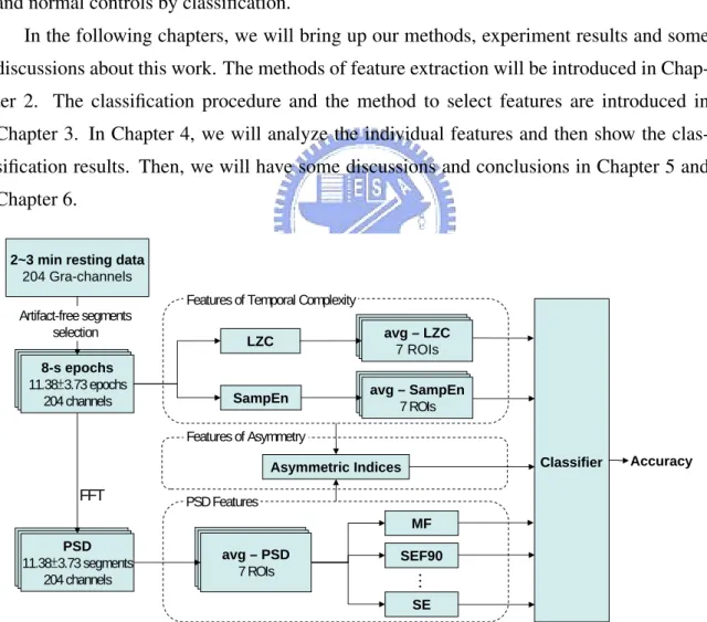
(26) 8. Introduction. 1.4. Thesis Scope. The objective of this thesis is to differentiate the patients with mood disorders from the healthy controls by the resting MEG signals. Fig. 1.1 illustrates the framework of this thesis. We preprocess the MEG signals and then extract features from them. There are three kind of features. The first is the PSD features which extract from the power spectral density, the second is about temporal complexity, and the other one is hemispheric asymmetry. The features of hemispheric asymmetry are calculated from the features of PSD and temporal complexity. Finally, those features are used to differentiate the BD patients, MDD patients and normal controls by classification. In the following chapters, we will bring up our methods, experiment results and some discussions about this work. The methods of feature extraction will be introduced in Chapter 2. The classification procedure and the method to select features are introduced in Chapter 3. In Chapter 4, we will analyze the individual features and then show the classification results. Then, we will have some discussions and conclusions in Chapter 5 and Chapter 6. 2~3 min resting data 204 Gra-channels Artifact-free segments selection 8-s 8-s epochs 8-sepochs epochs 11.38±3.73 11.38±3.73 epochs 11.38±3.73epochs epochs 204 204 channels 204channels channels. Features of Temporal Complexity LZC. avg –– SampEn avgavg SampEn – LZC 777ROIs ROIs ROIs. SampEn. avg avg SampEn avg–––SampEn SampEn 777ROIs ROIs ROIs. Features of Asymmetry Classifier. Asymmetric Indices. FFT. PSD Features MF avg avg PSD avg–––PSD PSD 777ROIs ROIs ROIs. SEF90. …. 8-s 8-s epochs epochs PSD 11.38±3.73 epochs 11.38±3.73segments epochs 11.38±3.73 204 204 channels 204channels channels. SE. Figure 1.1: Framework.. Accuracy.

(27) Chapter 2 Feature Extraction.

(28) 10. Feature Extraction. This chapter is concerning how we extract features to differentiate different groups based on some abnormalities of brain function. There are three kind of features used in this work. The first is the PSD features in section 2.2, the second is the features about temporal complexity in section 2.3, and the last is about the hemispheric asymmetry of the brain.. 2.1. ROI. According to the function of brain, we divided the brain into seven areas: frontal, central, occipital, left frontotemporal, right frontotemporal, left temporal and right temporal. Discarding the channels in the suburbs of the brain where the activities are rarely weak, we divided the MEG channels into seven groups according to the seven areas mentioned above. The seven groups of MEG channels are shown in Fig. 2.1. Besides the seven channels groups, we also observe the whole brain activities by the union of the seven channel groups. In another word, we analysis the brain in eight different ROIs: the seven areas separately and the union of the seven areas.. 2.2. PSD features. In this work, we used several spectral based measures to summarize the information of the power spectral density (PSD).. 2.2.1. Band Powers. The frequency bands are defined as delta (2-4 Hz), theta (4-8 Hz), alpha (8-13 Hz), beta (13-30 Hz) and gamma (30-50 Hz). The power spectrum density is first normalized by the total power, the areas under PSD curve. And then each band power is calculated from the average of the power bins within the same frequency band..

(29) 2.2 PSD features. 11. Central Right frontotemporal Right temporal Occipital. Frontal Left frontotemporal Left temporal 29. 18. 31. 17. 32 30. 19. 9. 34. 43. 20. 33. 2. 51. 36. 10. 6. 5. 44. 45 11. 3. 35. 21 12. 1. 13. 14. 52. 46. 22. 24. 37. 23. 38. 25. 26. 47. 40. 39. 48. 54 53. 4 16. 7. 15. 42. 41. 50. 8. 55. 68. 67. 60. 58. 59 56. 28. 27. 69. 86. 83. 84. 70. 91. 100 102. 85 94 75. 62. 76. 93. 71 78. 74 72. 65. 101. 87. 64. 63. 99. 92. 61 57. 49. 77. 96 88. 90. 79. 73. 95. 97. 89 80. 66 82. 98 81. Figure 2.1: Schematic illustration of the MEG sensor layout and the ROIs. In this work, we devide the brain into 7 areas: frontal, central, occipital, left frontotemporal, right frontotemporal, left temporal and right temporal. The illustration shows the channel groups corresponding to the 7 areas. Different colors are used to distinguish different areas, and the gray channels in the suburbs of the brain are discarded due to the weak activitis.. 2.2.2. Spectral Measures. Mean frequency (MF) offers a simple means which summaries the whole power spectrum. It is defined as the frequency which contains 50% of the PSD power. As a frequency which divides PSD into equal powers, the mean frequency can roughly present the trend of band power distribution. The mean frequency is represented in Eq. 2.1, where MF is calculated from the PSD between 2 Hz and 50 Hz. It has been used to study the spectrum of Alzheimer’s disease, mild cognitive impairment or vascular dementia patients’ EEG or MEG signals [15, 31]..

(30) 12. Feature Extraction. Figure 2.2: Schematic representation of MF and SEF90 [44]. The median frequency (MF) is the freqeuncy that divides the area under the curve in half, and the 90% spectral edge frequency (SEF90) is the frequency which divides the area area into 90% and 10%.. 0.5. 50Hz X. PSD(f ) =. MF X. PSD(f ).. (2.1). f =2Hz. f =2Hz. Similar to the mean frequency, the 90% spectral edge frequency (SEF90) is defined as the frequency which separates 90% of the PSD power from 10%. It has been used to study monitor depth of anaesthesia and Alzheimer’s disease. Eq. 2.2 represents the calculation of SEF90 which is analogous to the mean frequency shown in Eq. 2.1.. 0.9. 50Hz X. P SD(f ) =. f =2Hz. SEF X90. P SD(f ).. (2.2). f =2Hz. Fig. 2.2 shows the concept of MF and SEF90. The MF divides the area under the PSD curve into equal parts, and the SEF90 divides the area into 90% and 10% parts.. 2.2.3. Spectral Ratio Measures. To calculate the spectral ratio measures is a method to emphasize the difference between the powers of high and low frequency bands..

(31) 2.2 PSD features. 13. Some previous EEG studies successfully used the spectral ratio measures to distinguish between patients of cognition disorders and Alzheimer’s disease [24,27]. Some other studies also use the ratio to emphasize the difference between Alzheimer’s disease and elderly normal controls [8, 32, 38]. Poza used four spectral ratios to differentiate the patients of Alzheimer’s disease from the normal controls. And the spectral ratios reveal the higher correlation with severity of dementia than individual relative band powers. According to the characteristics of the Alzheimer’s disease, Poza evaluate the power ratio of high frequency to low frequency bands shown in Eq. 2.3 to Eq. 2.6 where relative power was calculated in the frequency bands: δ (1-4 Hz), θ (4-8 Hz), α (8-13 Hz), β1 (13-19 Hz), β2 (19-30 Hz) and γ (30-64 Hz) [32]. RP (α) . RP (θ). (2.3). RP (α) + RP (β1 ) + RP (β2 ) + RP (γ) . RP (δ) + RP (θ). (2.4). RP (β1 ) + RP (β2 ) . RP (δ). (2.5). RP (β2 ) . RP (δ). (2.6). r1 =. r2 =. r3 =. r4 =. Due to the different characteristics of mood disorders, we designed different spectral ratio measures in this work. Based on the observed band power abnormalities of MDD patients, we used five spectral ratio measures defined in Eq. 2.7 to Eq. 2.11. rβγ2θα =. RP (β) + RP (γ) . RP (θ) + RP (α). (2.7). rβ2θ =. RP (β) . RP (θ). (2.8). rβ2α =. RP (β) . RP (α). (2.9).

(32) 14. Feature Extraction. 2.2.4. rγ2θ =. RP (γ) . RP (θ). (2.10). rγ2α =. RP (γ) . RP (α). (2.11). Spectral Entropy. Spectral Entropy is a method to quantify the flatness of the power spectral density (PSD). It applies the Shannon’s entropy computed over the normalized PSD. The entropy was first defined as a measure for information theory by Shannon [10], and it is a measure of the spread of the data. A data with a wider and flatter probability distribution will have higher entropy. On the contrary, a data with a narrower and pecked probability distribution will have lower entropy. As applying Shannon entropy to EEG and MEG signals, it quantifies the regularity and the spectral complexity of the time series. In the first, the PSD of the signal is computed. And then, the spectral entropy is calculated by using the amplitude components of the PSD of the signal as the probabilities in Shannon entropy calculations. In this work, we adopt two spectral entropies. The first type of spectral entropy is defined as Eq. 2.12 where PSDn (f ) denotes the normalized PSD of the total power between 2 Hz and 50 Hz.. SE = −. 50Hz X. P SDn (f )ln[P SDn (f )].. (2.12). f =2Hz. This definition of spectral entropy has been used to study anaesthesia monitor [7], the spectrum of Alzheimer’s disease [15, 31], and the detection of epilepsy [25]. The above-mentioned SE calculates all frequency bins of power spectral density, and it will be influenced by the different bandwidth. In other words, it brings about a bias in the frequency band with larger range. For example, the beta band (13-30 Hz) will have lager weight than theta band (4-8 Hz) due to the bandwidth. Poza brought up the second type of spectral entropy to analyze Alzheimer’s disease [30]..

(33) 2.3 Temporal Complexity. 15. To calculate the second type of spectral entropy (SE2), we denote the average power at each frequency band as Pj , j = {δ, θ, α, β, γ}. Then we normalize the average power by the sum of them as Eq. 2.13 where pj represent the probability distribution of each band. AP (j) . pj = P j AP (j) Afterwards, we apply Shannon’s entropy as Eq. 2.14 . SE2 = −. X. pj · ln[pj ].. (2.13). (2.14). j. 2.3. Temporal Complexity. 2.3.1. Lempel-Ziv Complexity. The Lempel-Ziv complexity (LZC) proposed by Lempel and Ziv is a nonparametric method to evaluate complexity (randomness) of finite sequences [3]. The LZ complexity measures the number of distinct substrings and the rate of their occurrence along the given sequence. The more complex data will have larger values. Lempel-Ziv complexity has been widely used to solve information theoretic problems and applied to data compression [1,23] and coding [5,42]. In recent years, the LZC has been applied to biomedical signal analysis as a measurement of the complexity of discrete time signals. For example, the LZC was used to evaluate the complexity of DNA sequences [21], and to differentiate different kinds of stimuli [41]. Besides, LZC has also been used to study the Alzheimer’s disease [14, 19], epileptic seizure time-series data [33], the depth of anesthesia [46], and the intracranial pressure signals with acute intracranial hypertension episodes [2]. LZ complexity analysis is based on a coarse-graining of the measurements [46]. In other words, before calculating the LZ complexity, the signal must be transformed into a sequence whose elements are only a few symbols. In this work, we convert the MEG signal x = [x1 , x2 , . . . , xN ] into a binary sequence. By comparison with the threshold Td , the original signal x is converted to a binary sequence P = [s1 , s2 , . . . , sN ] where si is defined by:.

(34) 16. Feature Extraction.  0 if xi < Td si = 1 otherwise. (2.15). We use the median as the threshold Td because of it is robust to outliers [29]. To calculate the LZ complexity, the sequence P is scanned from left to right, and the subsequence number c(N ) is increase by one while a new substring was found. The algorithm of Lempel-Ziv complexity analysis is as follows. Let S and Q denote subsequence of the sequence P = [s1 , s2 , . . . , sN ], and SQ be the concatenation of S and Q. Let π be a operation which deletes the last character in a sequence, and then SQπ is a substring derived from sequence SQ with its last character deleted. And then, let ν(SQπ) denote the vocabulary of all different subsequences of SQπ. Initially, we set the subsequence number c(N ) = 1, S = s1 , Q = s2 , and therefore SQπ = s1 . In general, we suppose S = s1 , s2 , . . . , sr , Q = sr+1 , and SQπ = s1 , s2 , . . . , sr . And then, there are two cases: 1. If Q ∈ ν(SQπ), then Q is a subsequence of SQπ. In other words, Q is not a new sequence. In this case, S dose not change and Q is renewed to be sr+1 , sr+2 , . . . , sr+i until Q ∈ / ν(SQπ). 2. If Q ∈ / ν(SQπ), then Q is not a subsequence of SQπ. In this case, c(N ) increases by one and S is renewed by combining original S with Q. At this time, S is s1 , s2 , . . . , sr , sr+1 , . . . , sr+i and Q is renewed with Q = sr+i+1 . Repeat the procedure until Q is the last character. At this time, the number of different subsequences c(N ) is the measurement of LZ complexity. The last step of the procedure is to normalize c(N ) in order to obtain a complexity measure independent of the sequence length. Suppose the number of different symbols is α and the sequence length is N . It has been proved that the upper bound of c(N ) [3] is. lim c(N ) = b(N ) =. N →∞. For a binary sequence, α = 2, therefore. N logα N. (2.16).

(35) 2.3 Temporal Complexity. 17. Figure 2.3: LZC concept. An example showing how to transform a segment of time series into a binary sequence by threshold and the results of LZC calculation [46].. b(N ) =. N log2 N. (2.17). and c(N ) can be normalized by the upper bound b(N ) as C(N ) =. c(N ) b(N ). (2.18). Fig. 2.3 illustrates the example of calculating LZC. The time series will first trnasform into a binary series and then a LZC procedure is appled to calculate the LZC values.. 2.3.2. Sample Entropy. Sample Entropy (SampEn) quantifies the regularity of a time series by evaluation the appearance of repetitive patterns. It has already been widely used to study some biomedical signals. For example, it was applied to representative interbeat interval time series and differentiate subjects with congestive heart failure and atrial fibrillation from healthy subjects [13]..

(36) 18. Feature Extraction To calculate the sample entropy of x, there are two parameters: m and r. m is the. length of sequences to be compared, and r is the tolerant range of match. Given a time series x = [x1 , x2 , . . . , xN ] with length N . First form vectors Xm (1), Xm (2), . . . , Xm (N − m + 1) with length of m, and let Xm (i) = [xi , xi+1 , . . . , xi+m−1 ]. Then define the distance d[Xm (i), Xm (j)] between vectors Xm (i) and Xm (j) as the maximum difference in their respective scalar components. d[Xm (i), Xm (j)] =. max (kxi+k−1 − xj+k−1 k).. k=1,2,...,m. (2.19). Define Bim (r) as 1/(N − m − 1) times the number of vectors Xm (j) within r of Xm (i) (the distance between Xm (j) and Xm (i) is less than or equal to r) where 1 ≤ j ≤ N − m(j 6= i) to exclude self-matches. Then define Bm (r) as: N −m X 1 Bm (r) = Bim (r) N − m i=1. (2.20). Similarly, define Am i (r) as 1/(N − m − 1) times the number of Xm+1 (j) such that the distance between Xm+1 (j) and Xm+1 (i) is less than or equal to r. And then set Am (r) as:. Am (r) =. N −m X 1 Am (r) N − m i=1 i. (2.21). Finially, SampEn(m, r) is defined by:. SampEn(m, r) = lim [− ln N →∞. Am (r) ] Bm (r). (2.22). which is estimated by the statistic. SampEn(m, r, N ) = − ln. 2.3.3. Am (r) Bm (r). (2.23). Multi-Scale Entropy. The entropy-based measurements quantify the regularity of a time series. In theory, an increase in entropy represents the increase of complexity. However, it may not always be.

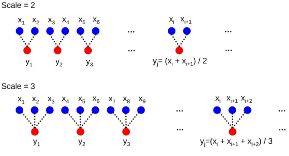
(37) 2.3 Temporal Complexity. 19. Scale = 2 x1 x2. y1. x3 x4. xi xi+1. x5 x6 …. …. …. … yj= (xi + xi+1) / 2. y2. y3. x3 x4. x5 x6. Scale = 3 x1 x2. y1. x7 x8. y2. xi xi+1 xi+2. x9 …. …. …. …. y3. yj=(xi + xi+1 + xi+2) / 3. Figure 2.4: the concept of sample entropy. xzz.. true in real case. One possible reason may be the fact that these measures are based on a single scale [12]. Costa brought up a multiscale method based on the sample entropy, and it is a non-linear method to measure complexity over a range of scales [12]. The MSE procedure is as follows [12,18]. Given a discrete time series x = [x1 , x2 , . . . , xN ], τ consecutive coarse-grained time series y τ = [y1τ , y2τ , . . . , yN/τ ] is constructed corresponding. to the scale factor τ . In the first place, the original time series x is divided into nonoverlapping windows of length τ . Second, we average the data points within the same window according to Eq. 2.24. Fig. 2.24 illustrates this coarse-grained method. Afterwards, sample entropy for each coarse-grained sequences is calculated and plotted as a function of the scale factor.. yjτ. 1 = τ. jτ X i=(j−1)τ +1. x1 , 1 ≤ j ≤. N τ. (2.24).

(38) 20. Feature Extraction. 2.4. Hemispheric Asymmetry. Hemispheric EEG activation asymmetry in the patients with mood disorders has been frequently observed in recent years as mentioned in section 1.2.3. Knott measured the inter-hemispheric absolute power asymmetry for each band in eight homologous sites (Fp1-Fp2, F7-F8, F3-F4, C3-C4, P3-P4, O1-O2, T3-T4, T5-T6) [26]. In Knott’s method, the activity asymmetric indices of left hemisphere (L) and right hemisphere (R) were calculated with the formula: L−R L+R. (2.25). In this work, we follow the basic comparison method as Eq. 2.25 but change the sitebased comparison. Unlike the EEG channels, the amount of MEG channels is bigger and the channels are closed to each other. For this reason, differ from EEG studies, we compare the brain asymmetry region by region shown in Fig. 2.5. Based on the ROIs mentioned in section 2.1, we slightly modify the ROI design. In the middle areas (frontal, central and occipital), we discard the channels directly on the midline of the brain and divide the other channels into left and right groups. The left and right temporal areas are in pairs, but we subdivide frontotemporal areas into lateral and interior parts due to the bigger channel number. In other words, the left lateral- and interior- frontotemporal areas are corresponding to right lateral- and interior- frontotemporal areas respectively. Besides the band power asymmetry, we also extend the asymmetric indices to other features described in section 2.2 and section 2.3..

(39) 2.4 Hemispheric Asymmetry. 21. Frontal Lateral frontotemporal Interior frontotemporal 29. 18. 31. 17. 32 30. 19. 9. 34. 43. 20. 33. 2. 51. 36. 10. 6. 5. 44. 45 11. 3. 35. 21 12. 1. Central Temporal Occipital. 13. 14. 52. 46. 22. 24. 37. 23. 38. 25. 26. 47. 40. 39. 48. 54 53. 4 16. 7. 15. 42. 41. 50. 8. 55. 68. 67. 60. 58. 59 56. 28. 27. 69. 86. 83. 84. 70. 91. 100 102. 85 94 75. 62. 76. 93. 71 78. 74 72. 65. 101. 87. 64. 63. 99. 92. 61 57. 49. 77. 96 88. 90. 79. 73. 95. 97. 89 80. 66 82. 98 81. Figure 2.5: Schematic illustration of the MEG sensor layout and the ROIs for asymmetric analysis. There are six areas for observation: frontal, central, occipital, lateralfrontotemporal, interior-frontotemporal and temporal. The illustration shows the channel groups corresponding to the six areas, and the same colors stand for the areas in pairs. The gray channels were excluded due to the week activitis or right in the middle of the brain..

(40) 22. Feature Extraction.

(41) Chapter 3 Classification.

(42) 24. Classification. This chapter is concerning how we select the features with differentiability and design the classifier. In the following sections, the methods of t-test and Linear Discriminant Analysis (LDA) are applied to select beneficial feature for classification. And then the classification will be brought out by Support Vector Machine (SVM) described in section 3.2. Fig. 3.1 shows the classification procedures in this work.. All Features Feature Selection T-Test p < 0.03 Features Reaching a significant level LDA Features With large weighting Dimension Reduction Projection Features With low dimensionality Classification SVM Leave-one-out validation Classification Result Accuracy = ?. Figure 3.1: Classification procedures. The figure shows the classification procedures in this work. The significant level of t-test is set to be the first threshold to select features in the first place. And then the features selected from t-test are selected again by LDA method. To reduce the dimensionality of feature set, we then project the selected features to a subspace with low dimension by LDA projection matrix. Finally, SVM is applied to classify the final features..

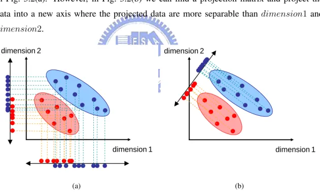
(43) 3.1 Linear Discriminant Analysis. 3.1 3.1.1. 25. Linear Discriminant Analysis Introduction to LDA. Linear discriminant analysis (LDA) is one of the most popular techniques for data classification and dimensionality reduction. It was originally developed in 1936 by R.A. Fisher [17], and has been widely applied in the areas of classification, face recognition, marketing researches. The LDA method finds the linear combination of features which best separate two or more classes and the resulting combination may be used as a linear classifier or for dimensionality reduction before classification. Fig. 3.2 illustrates a simple idea for LDA projection. It is an example of two dimensional data, and the data is unable to be separated by neither dimension1 nor dimension2 in Fig. 3.2(a). However, in Fig. 3.2(b) we can find a projection matrix and project the data into a new axis where the projected data are more separable than dimension1 and dimension2. dimension 2. dimension 2. dimension 1. (a). dimension 1. (b). Figure 3.2: An idea of LDA projection. The figure shows an example of LDA in two dimensions. The data can not be separate from each other in any of the two axes in (a). However we may project data into another one dimension axis which is the combination of the original axes and the projected data is be more separable in (b). Let K be the number of classes, N be the number of all samples where Nk is the number.

(44) 26. Classification. of samples in the kth class. The within-class scatter matrix Sw and the between-class scatter matrix Sb are defined as Sw =. K X. X. (x − µk )(x − µk )T ,. (3.1). k=1 x∈Class k. and Sb =. K X. Nk (µk − µ0 )(µk − µ0 )T ,. (3.2). k=1. where µk is the mean vector of the kth class, and µ0 is the global mean vector defined as µ0 =. K 1 X Nk µ k . N k=1. (3.3). The objective of LDA is to find a projection matrix P which projecting the feature vectors onto a l-dimensional subspace of the original m-dimensional feature space and the projected feature vectors maximizes the Fisher’s discriminant ratio. The Fisher’s discriminant criterion is J = tr{Sw −1 Sb }.. (3.4). Thus the objective function can be written as PLDA = arg max J = arg max P. P. P T Sb P P T Sw P. (3.5). According to the linear algebra, we get Sw −1 Sb P = λP,. (3.6). where the column vectors of projection matrix PLDA are the eigenvectors of Sw −1 Sb . In case of K classes, LDA can reduce dimensionality to 1, 2, . . . , K − 1 dimensions. In the 2-classes case, the vector Sb P is always along the (µ1 − µ2 ) direction, and we can then obtain PLDA as Sw −1 (µ1 − µ2 ).. 3.1.2. Feature Selection. The performance of classifier depends on the interrelationship between the training sample size and the number of the features. To achieve an acceptable performance, the.

(45) 3.1 Linear Discriminant Analysis. 27. number of training samples grows exponentially with the dimensionality of features [35]. This phenomenon is termed as curse of dimensionality, which leads to the peaking phenomenon in classifier design and impacts on the performance of the classifier. In practice, it has been observed that the added features may degrade the performance of a classifier if the number of the training samples is small relative to the number of the features used for clasification [6]. Therefore, for a fixed sample size, it is necessary to reduce the number of features to a sufficient minimum. In this work, we use t-test to select the most discrepant features and apply LDA to reduce the dimensionality of feature set. Fig. 3.3 is an example of different importances in different dimensions. With LDA, we can project data to a subspace with low dimension and it is obviously that dimension 2 contribute more than dimension 1 to the projection. It means that dimension 2 is probably more important than dimension 1 for classification. Thus we select the features with larger weightings in the projection matrix of LDA in order to get the features favorable for classification.. dimension 2. dimension 1. Figure 3.3: The weighting of LDA projection matrix..

(46) 28. Classification. L2. L2. L1. L1. xB. Class B. Class A. Class B. Class A. (a). xA. (b). Figure 3.4: The idea of selecting separating hyperplain in SVM. The circles represent the samples, and different color represent for different groups. In (a), both L1 and L2 can separate class A from class B successfully. In (b), L1 can separate two classes correctly but L2 does not, while considering with new sample xA in class A and xB in class B.. 3.2. Support Vector Machine. Support Vector Machine (SVM) is a powerful method of classification. In recent years, SVM has been applied to diverse problems very successfully, such as face recognition. The main idea of SVM is to determine a decision hyperplane which not only separates different groups, but also be as far as possible from all samples. Fig. 3.4 depicts this idea. When considering only the training set just like Fig. 3.4(a), both the two hyperplane L1 and L2 can separate class A from class B well. However, when considering with the new testing sample xA and xB in Fig. 3.4(b), L2 fail to classify xA to class A even though xA is close to one of the samples in class A and so does xB and class B. The SVM method decides which hyperplane separates classes generally, that is, the hyperplane with largest margin, which is as far as possible from all samples like L1 in Fig. 3.4. The margin is defined as twice the absolute value of distance of the closest samples to the separating hyperplane as Fig. 3.5. The samples closest to the separating hyperplane are defined as support vectors and which completely define the optimal hyperplane. Let the separating hyperplane be wT x + w0 , and then the distance between sample x and the.

(47) 29. 2/ rg ||w in ||. w. w. m a. m ar gi n. 3.2 Support Vector Machine. support vector. |w. Class B. T. w. =1 0 +w Tx =0 0 w +w Tx w 1 =w0 x+. 1/|. |w. ne =0 la rp +w 0 pe T x hy w. Class A. 1/|. Class B. ||. g tin ra pa Se. ||. support vector. Class A. (a). (b). Figure 3.5: Margin and support vectors of SVM. The figure shows an example of a linear SVM for two classes. (a)The samples with black edges are the support vectors, which are the closest samples to the separating hyperplane. (b)The distance from support vectors to the largest margin hyperplane is 1/||w||, and the margin is 2/||w||. hyperplane is given by |wT x + w0 | . ||w||. (3.7). The distance is unchanged after scaling w and w0 . Thus to make the largest margin hyperplane is unique, we add the requirement to support vectors: |wT x + w0 | = 1.. (3.8). And then, the distance from support vectors to the largest margin hyperplane is 1/||w||, and the margin is given by 2/||w|| as depicted in Fig. 3.5(b). The objective of SVM is to maximize the margin 2/||w|| subject to the constraints  w T xi + w 0 ≥ 1 if xi is a positive example. wT x + w ≤ −1 if x is a negative example. i 0 i. (3.9).  yi = 1 if xi is a positive example. y = −1 if x is a negative example. i i. (3.10). Let.

(48) 30. Classification. Then can convert the problem to minimize 1 J(w) = ||w||2 2. (3.11). yi (wT xi + w0 ) ≥ 1, ∀i.. (3.12). constrained to. Using Lagrange multipliers λi to include the constraints: N. X 1 L = ||w||2 − λi [yi (wT xi + w0 ) − 1], 2 i=1. (3.13). then minimize L relative to w and w0 by setting the partial derivatives to zero and get w=. N X. λi y i xi. (3.14). i=1 N X. λi yi = 0. (3.15). i=1. Substitude Eq. 3.14 an Eq. 3.15 into Eq. 3.13, then the problem is transformed to maximize L=. N X i=1. N. N. 1 XX λi λj yi yj xi T xj . λi − 2 i=1 j=1. (3.16). Subject to the constraints N X. λi yi = 0 and λi > 0, ∀i.. (3.17). i=1. By Cover’s Theorem, a pattern classification problem cast in a high dimensional space nonlinearly is more likely to be linearly separable than in a low-dimensional space. If we apply a transformation φ to all samples so as to lift the original feature spaces to a high dimensional spaces where the discriminability is stronger, then we can find a linear discriminant function for transformed data φ(x). Substitute φ into Eq. 3.16 L=. N X i=1. N. N. 1 XX λi λj yi yj [φ(xi )T φ(xj )]. λi − 2 i=1 j=1. (3.18). We define the kernal function K(xi , xj ) as K(xi , xj ) = φ(xi )T φ(xj ).. (3.19).

(49) 3.2 Support Vector Machine. 31. To substitute kernal function into Eq. 3.18, and we obtain L=. N X. N. λi −. i=1. N. 1 XX λi λj yi yj K(xi , xj ). 2 i=1 j=1. (3.20). Various kernal function choices have been brought up such as Gaussian radial basis kernal. Gaussian radial basis kernal is K(xi , xj ) = exp(−. ||x − z||2 ). 2σ 2. (3.21). where the σ adjusts the smoothness of the boundary. Such kernal based support vector machine is often a nonlinear SVM method..

(50) 32. Classification.

(51) Chapter 4 Experiment Results.

(52) 34. Experiment Results. In this chapter, we show the experiment results in this work. We first introduce the materials used in the experiment, and than show the differences between three groups about every feature. According to the analysis of each feature, a corresponding classifier was designed and trained with real data. Finally we show the classification accuracy of these groups. Further discussions and conclusions will be provided in the next chapter.. 4.1 4.1.1. Materials Subjects. In this work, three study groups are collected, including normal controls (NC), bipolar disorder (BD), and major depressive disorder (MDD). Patients with BD and MDD were selected from the outpatients of psychiatric department of Taipei Veterans General Hospital, and the clinical diagnosis was made by two independent psychiatrists according to DSM-IV criteria. Demographic data of all subjects are summarized in Table 4.1. The BD group consisted of 26 patients suffering from bipolar disorder, and the MDD group consisted of 22 patients with major depressive disorder. 25 healthy subjects, matched by age and without history of any psychiatric disorders and neurological disorders, were recruited through advertisement from the community. Besides, all of the normal controls underwent Mini International Neuropsychiatric Interview (M.I.N.I.) before the experiments to exclude the possible morbidity of major psychiatric illness. All subjects provided written informed consent to participate in the experiment and study according to the guidelines approved by the Institutional Committees of Medical Ethics and Radiation Safety.. 4.1.2. MEG Device. The minute magnetic field generated by electrical activity within the living human brain was measured with a whole-head MEG system at Integrated Brain Research Unit of Taipei Veterans General Hospital (Neuromag Vectorview 306, Neuromag Ltd., Helsinki, Finland.) The MEG system contains 204 gradiometer sensors and 102 magnetometer sensors which simultaneously record at 102 distinct sites covering the entire scalp. The system has the.

(53) 4.1 Materials. 35. Figure 4.1: MEG device. The MEG device in Integrated Brain Research Unit of Taipei Veterans General Hospital.. capabilities of 24 bits analog to digital conversion and up-to-8 kHz sampling rate which is sufficient to probe the fast dynamic changes inside human brains. Figure 4.1 shows the MEG device.. Table 4.1: Demographic data of subjects. The table shows the demographic data of the three groups: normal controls (NC), patients with bipolar disorder (BD), and patients with major depressive disorder (MDD). Variable. NC. BD. MDD. n. 25. 26. 22. Gender, n(%), male. 9 (36.00). 10 (38.46). 8 (36.36). Age, mean (SD), years. 36.04 (11.19). 34.62 (10.40). 34.18 (9.17). Handedness, n(%), right. 25 (100). 26 (100). 21 (95.45).

(54) 36. Experiment Results. 4.1.3. MEG Data Collection. Data recording was performed in a magnetically shielded room (Euroshield, Eura, Finland) at Integrated Brain Research Unit of Taipei Veterans General Hospital. The magnetic fields were recorded while subjects were seated comfortably and in a resting state, relax, awake, and with eyes closed for two to three minutes. The signals were recorded at a sampling rate of 1001.6 Hz and was filtered with a bandwidth of 0.03-330 Hz.. 4.2. Data Preprocessing. The brain signal is relative weak as compared with environmental interference noises. To extract the weak brain signals, experiment should be in a magnetically shielded room. Besides, in order to enhance signal-to-noise ratio (SNR), some preprocessing procedure is necessary before the further processing. The preprocessing steps we used for MEG recordings are as follows and shown in Figure 4.2. First, we eliminate bad channels which record abnormally. Second, while conducting experiment, eye movement and eye blinking may contaminate the MEG signals. To avoid the noise, we found out the abnormal scale of Electro-OculoGram (EOG) manually. Only the segments without eye blinking and eye movement were accepted for further analysis. Third, signal space projection (SSP) was applied to eliminate the ambient noise. Furthermore, because the MEG recording may drift along with time due to the device, a baseline correction was applied in each channel. The baseline is estimated by the mean of the whole segment. Besides eye movement and eye blinking, there are still some external artifacts like heartbeat, breath, and electromyographic(EMG). Therefore, finally we use bandpass filter of 2-50 Hz to minimize those unavoidable artifacts. Only the signals recorded from gradiometer sensors were used in this study, because gradiometer sensors detect less ambient noise and give the largest signal right above the source [28]..

(55) 4.3 Features of Power Spectrum. Recording. Bad-channel Elimination. Epoch Segmentation. 37. SSP. Baseline Correction. Bandpass Filtering. EOG Detection. Figure 4.2: Preprocessing procedures for MEG recordings. In order to enhance SNR, preprocessing for the recordings is necessary before the further processing. First we eliminate the bad channels and choose the segmentations without eye movements for further analysis. Second, we apply signal space projection (SSP) to eliminate the unbalanced noise effect on different sensors. Then baseline correction is applied to eliminate the drift of recordings. Finally, a 2-50 Hz bandpass filter is used to eliminate other artifacts such as heartbeat and breath.. 4.3. Features of Power Spectrum. To characterize the spectral content of each MEG recording, we used the Fourier transform and then extracted the features. Initially, we computed the power spectral density (PSD) for each epoch and then averaged the PSD for all epochs. To compare with different area of brain, we averaged the PSD of different channels based on the ROI showed in section 2.1.. 4.3.1. band power. Fig. 4.3 shows the relative band powers of the five frequency bands, and Table 4.2, Table 4.3 and Table 4.4 show the p-value of two groups comparisons. Compared with the three groups, the delta band power of the patients with bipolar disorder are slightly stronger than others and so do the alpha band power of normal controls. However, these differences do not reach the significant level (p-value < 0.05). On the other hand, the beta and gamma band powers of patients with major depressive disorder are stronger significantly, especially than the normal controls..

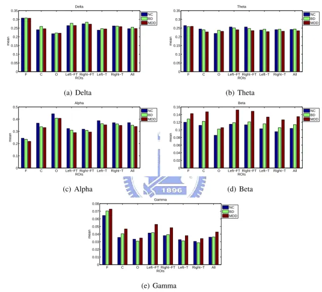
(56) 38. Experiment Results. Delta. Theta. 0.35. 0.35 NC BD MDD. 0.3. 0.25. 0.2. mean. mean. 0.25. 0.15. 0.2 0.15. 0.1. 0.1. 0.05. 0.05. 0. NC BD MDD. 0.3. F. C. O. Left−FT Right−FT Left−T ROIs. Right−T. 0. All. F. C. O. (a) Delta. Left−FT Right−FT Left−T ROIs. All. (b) Theta. Alpha. Beta. 0.5. 0.16 NC BD MDD. 0.4. NC BD MDD. 0.14 0.12 0.1. 0.3. mean. mean. Right−T. 0.2. 0.08 0.06 0.04. 0.1. 0.02 0. F. C. O. Left−FT Right−FT Left−T ROIs. Right−T. 0. All. F. C. O. (c) Alpha. Left−FT Right−FT Left−T ROIs. Right−T. All. (d) Beta Gamma. 0.08 NC BD MDD. 0.07 0.06 mean. 0.05 0.04 0.03 0.02 0.01 0. F. C. O. Left−FT Right−FT Left−T ROIs. Right−T. All. (e) Gamma. Figure 4.3: Relative band power. The bar chart shows the relative band power in the NC, BD and MDD groups..

(57) 4.3 Features of Power Spectrum. 39. Table 4.2: The p-values of band power between NC and BD. The differences between normal controls (NC) and patients with bipolar disorder (BD) are not significant in any frequency bands. Variable. Frontal. Central. Occipital. Frontotemporal. Temporal. Left. Right. Left. Right. All. Delta. 0.979. 0.417. 0.853. 0.566. 0.675. 0.718. 0.961. 0.696. Theta. 0.452. 0.754. 0.367. 0.734. 0.561. 0.783. 0.898. 0.874. Alpha. 0.609. 0.435. 0.383. 0.671. 0.761. 0.495. 0.791. 0.537. Beta. 0.131. 0.379. 0.165. 0.733. 0.512. 0.341. 0.356. 0.373. Gamma. 0.126. 0.239. 0.549. 0.883. 0.765. 0.663. 0.566. 0.942. Table 4.3: The p-values of band power between NC and MDD. Compared with NC, the relative band power of patients with major depressive disorder (MDD) are quite different in beta and gamma band, especially in the beta band power of frontal, gamma band power of central and frontotemporal of brain. Variable. Frontal. Central. Occipital. Frontotemporal. Temporal. Left. Right. Left. Right. All. Delta. 0.954. 0.778. 0.888. 0.959. 0.927. 0.723. 0.850. 0.952. Theta. 0.617. 0.290. 0.530. 0.294. 0.178. 0.539. 0.540. 0.620. Alpha. 0.127. 0.334. 0.362. 0.233. 0.452. 0.318. 0.519. 0.321. Beta. 0.048. 0.056. 0.065. 0.077. 0.063. 0.069. 0.056. 0.059. Gamma. 0.061. 0.016. 0.731. 0.023. 0.023. 0.188. 0.271. 0.077.

(58) 40. Experiment Results. Table 4.4: The p-values of band power between BD and MDD. Compared BD with MDD, the significant difference of relative band power are in the gamma band of frontotemporal areas. Variable. Frontal. Central. Occipital. Frontotemporal. Temporal. Left. Right. Left. Right. All. Delta. 0.915. 0.564. 0.963. 0.585. 0.575. 0.956. 0.903. 0.730. Theta. 0.830. 0.386. 0.772. 0.466. 0.331. 0.375. 0.464. 0.491. Alpha. 0.187. 0.865. 0.984. 0.480. 0.630. 0.787. 0.728. 0.745. Beta. 0.215. 0.195. 0.804. 0.131. 0.154. 0.355. 0.258. 0.240. Gamma. 0.544. 0.178. 0.370. 0.032. 0.061. 0.113. 0.130. 0.096.

(59) 4.3 Features of Power Spectrum. 41. MF. SEF90. 20. 40 NC BD MDD. 15. NC BD MDD. 35 30 mean. mean. 25 10. 20 15. 5. 10 5. 0. F. C. O. Left−FT Right−FT Left−T ROIs. (a) Mean Frequency. Right−T. All. 0. F. C. O. Left−FT Right−FT Left−T ROIs. Right−T. All. (b) 90% spectral edge frequency. Figure 4.4: MF and SEF90. The bar chart shows the MF and SEF90 in all ROIs whithin the three groups. MF of patients with MDD apparently higher than that of NC and BD in all ROIs. But MF of BD patients and NC are quite similar. Compared MDD with NC, patients with MDD are still have a little higher SEF90 in each ROIs. But in the case of BD and MDD, SEF90 of BD are higher in frontal, central, and frontotemporal, but lower in others.. 4.3.2. MF and SEF90. Fig. 4.4 shows the bar chart of the mean frequency (MF) and the 90% spectral edge frequency (SEF90), and Table 4.5 and Table 4.3.2 show the detail of the p-value of the difference between any two groups. Roughly speaking, the MF and SEF90 of MDD are higher than NC and BD groups. The MF differences between NC and BD are not clear, but are significantly different between NC and MDD. Except for the occipital of brain, each ROI reaches significant level (p-value < 0.05). Compare the MF of BD with MDD, the frontotemporal has clearer differences, but only the left frontotemporal reaches significant level. On the contrary, the features of SEF90 do not show any clearer difference between any two groups..

(60) 42. Experiment Results. Table 4.5: The p-values of mean frequency (MF). The MF differences between NC and BD are unapparent, but significant between NC and MDD. Except for occipital, each ROI reaches significant level (p-value less than 0.05). Compare the MF of BD with MDD, the frontotemporal has clearer differences, but only the left frontotemporal reaches significant level. Variable. Frontal. Central. Occipital. Frontotemporal. Temporal. Left. Right. Left. Right. All. NC vs. BD. 0.158. 0.523. 0.690. 0.896. 0.878. 0.643. 0.878. 0.739. NC vs. MDD. 0.032. 0.018. 0.549. 0.028. 0.027. 0.020. 0.027. 0.016. BD vs. MDD. 0.249. 0.084. 0.233. 0.034. 0.051. 0.106. 0.106. 0.062. Table 4.6: The p-values of the 90% spectral edge frequency (SEF90). The significant differences of SEF90 are not found no matter what ROI is. Variable. Frontal. Central. Occipital. Frontotemporal. Temporal. Left. Right. Left. Right. All. NC vs. BD. 0.261. 0.233. 0.356. 0.882. 0.938. 0.364. 0.341. 0.912. NC vs. MDD. 0.337. 0.079. 0.982. 0.119. 0.104. 0.542. 0.554. 0.273. BD vs. MDD. 0.981. 0.501. 0.377. 0.132. 0.101. 0.135. 0.123. 0.195.

(61) 4.3 Features of Power Spectrum. 4.3.3. 43. Spectral Ratio Measures. Fig. 4.5 illustrates the means of the five spectral ratios described in section 2.2.3. In the MDD case, all means of these spectral ratios are larger than those of BD patients and NC group no matter what ROI is. The mean spectral ratios of patients with BD are almost larger than those of NC but smaller than those of MDD patients, besides some areas. The ratios of gamma to theta band in occipital and temporal are the smallest in the three groups, and so does the ratio of gamma band to alpha band. Table 4.3.3, Table 4.3.3 and Table 4.3.3 show the details of the p-values which show the degree of discrepancy between NC and BD, NC and MDD, and BD and MDD respectively. There are no obvious differences between NC and BD groups, but not between NC and MDD groups. The most different feature are the ratio of (RP (β) + RP (γ))/(RP (θ) + RP (α)) and the ROI of central of the brain. Ratio of (RP (β)+RP (γ))/(RP (θ)+RP (α)) in most ROIs are significant different between NC and MDD, besides occipital. Moreover, the ratio of gamma to theta band (RP (γ)/RP (θ)) reaches the strong significant level of p < 0.01 in central and right temporal of brain. Besides, in the case of comparison of BD and MDD patients, only the ratio of gamma to theta band (RP (γ)/RP (θ)) reach the significant level of p < 0.05. Table 4.7: The p-values of spectral ratios between NC and BD. In the NC and BD case, the spectral ratios do not differentiate BD from NC in any ROIs. Variable. RP (β)+RP (γ) RP (θ)+RP (α) RP (β) RP (θ) RP (β) RP (α) RP (γ) RP (θ) RP (γ) RP (α). Frontal. Central. Occipital. Frontotemporal. Temporal. Left. Right. Left. Right. All. 0.116. 0.190. 0.275. 0.543. 0.439. 0.316. 0.428. 0.333. 0.160. 0.365. 0.322. 0.461. 0.441. 0.297. 0.303. 0.378. 0.307. 0.168. 0.163. 0.458. 0.461. 0.203. 0.320. 0.227. 0.128. 0.200. 0.419. 0.612. 0.650. 0.880. 0.761. 0.875. 0.300. 0.119. 0.810. 0.497. 0.574. 0.717. 0.931. 0.494.

(62) 44. Experiment Results. rB2T. rB2A. 0.8. 0.7 NC BD MDD. 0.7 0.6. 0.5 mean. mean. 0.5 0.4 0.3. 0.4 0.3 0.2. 0.2. 0.1. 0.1 0. NC BD MDD. 0.6. F. C. O. Left−FT Right−FT Left−T ROIs. Right−T. 0. All. F. C. (a) RP (β)/RP (θ). O. Left−FT Right−FT Left−T ROIs. rG2A. 0.35. 0.35 NC BD MDD. 0.3. NC BD MDD. 0.3. 0.25. 0.25. 0.2. mean. mean. All. (b) RP (β)/RP (α). rG2T. 0.15. 0.2 0.15. 0.1. 0.1. 0.05. 0.05. 0. Right−T. F. C. O. Left−FT Right−FT Left−T ROIs. Right−T. 0. All. F. C. (c) RP (γ)/RP (θ). O. Left−FT Right−FT Left−T ROIs. Right−T. All. (d) RP (γ)/RP (α) rBG2TA. 0.5 NC BD MDD. mean. 0.4. 0.3. 0.2. 0.1. 0. F. C. O. Left−FT Right−FT Left−T ROIs. Right−T. All. (e) (RP (β) + RP (γ))/(RP (θ) + RP (α)). Figure 4.5: Spectral Ratios. The bar charts show five kinds of spectral ratios. For all spectral ratios, MDD patients have larger ratio means than NC and BD patients in all ROIs. All of the ratio means of BD patients are larger than those of NC and smaller than those of MDD, except for ratios of gamma to theta band in occipital and temporal areas and ratio of gamma to alpha band in occipital..