粒子群演算法於離散最佳化問題之研究

(1)

國立交通大學

工業工程與管理學系

博士論文

粒子群演算法於離散最佳化問題之研究

A Study on Particle Swarm Optimization for

Discrete Optimization Problems

研究生：徐誠佑

指導教授：沙永傑博士

陳文智博士

中華民國九十六年五月

(2)

粒子群演算法於離散最佳化問題之研究

A Study on Particle Swarm Optimization for Discrete

Optimization Problems

研究生：徐誠佑

Student： Cheng-Yu

Hsu

指導教授：沙永傑

Advisor： Dr. David Yung-Jye Sha

陳文智

Dr. Wen-Chih Chen

國立交通大學

工業工程與管理學系

博士論文

A Dissertation

Submitted to Department of Industrial Engineering and Management

College of Management

National Chiao Tung University

in Partial Fulfillment of the Requirements

for the Degree of

Doctor of Philosophy

in

Industrial Engineering and Managemen

May 2007

Hsinchu, Taiwan, Republic of China

(3)

粒子群演算法於離散最佳化問題之研究

學生：徐誠佑指導教授：沙永傑博士

陳文智博士國立交通大學工業工程與管理系

中文摘要

粒子群演算法(Particle Swarm Optimization, PSO)是一種群體搜尋最佳化演

算法，於 1995 年被提出。原始的 PSO 是應用於求解連續最佳化問題。當 PSO 用來求解離散最佳化問題時，我們必須修改粒子位置、粒子移動以及粒子速度的表達方式，讓 PSO 更適於求解離散最佳化問題問題。本研究之主要貢獻為提出數種適合求解離散最佳化問題之 PSO 設計。這些新的設計和原始的設計不同且更適合求解離散最佳化問題。在本篇論文中，我們將分別提出適合求解零壹多限制式背包問題

(Multidimensional 0-1 Knapsack Problem, MKP) 、零工式排程問題 (Job Shop

Scheduling Problem JSSP)以及開放式排程問題(Open Shop Scheduling Problem,

OSSP)的 PSO。在求解 MKP 的 PSO 中，我們以零壹變數表達粒子位置，以區塊建立(building blocks)的概念表達粒子移動方式。在求解 JSSP 的 PSO 中，我們以

偏好列表(preference-list)表達粒子位置，以交換運算子(swap operator)表達粒子移

動方式。在求解 OSSP 的 PSO 中，我們以優先權重(priority)表達粒子位置，以插

入運算子(insert operator)表達粒子移動方式。除此之外，我們在求解 MKP 的 PSO

中加入區域搜尋法(local search)，在求解 JSSP 的 PSO 與塔布搜尋(tabu search)混

合，以及將求解 OSSP 的 PSO 與集束搜尋法(beam search)混合。計算結果顯示，

我們的 PSO 比其它傳統的啟發式解法要來的好。

關鍵字：粒子群演算法、零壹多限制式背包問題、零工式排程問題、開放式排程

(4)

A Study on Particle Swarm Optimization for Discrete

Optimization Problems

Student：Cheng-Yu Hsu Advisor： Dr. David Yung-Jye Sha Dr. Wen-Chih Chen Department of Industrial Engineering and Management

National Chiao Tung University

ABSTRACT

Particle Swarm Optimization (PSO) is a population-based optimization algorithm, which was developed in 1995. The original PSO is used to solve continuous optimization problems. Due to solution spaces of discrete optimization problems are discrete, we have to modify the particle position representation, particle movement, and particle velocity to better suit PSO for discrete optimization problems. The contribution of this research is that we proposed several PSO designs for discrete optimization problems. The new PSO designs are better suit for discrete optimization problems, and differ from the original PSO.

In this thesis, we propose three PSOs for three discrete optimization problems respectively: the multidimensional 0-1 knapsack problem (MKP), the job shop scheduling problem (JSSP) and the open shop scheduling problem (OSSP). In the PSO for MKP, the particle position is represented by binary variables, and the particle movement are based on the concept of building blocks. In the PSO for JSSP, we modified the particle position representation using preference-lists and the particle movement using a swap operator. In the PSO for OSSP, we modified the particle position representation using priorities and the particle movement using an insert operator. Furthermore, we hybridized the PSO for MKP with a local search procedure, the PSO for JSSP with tabu search (TS), and the PSO for OSSP with beam search (BS). The computational results show that our PSOs are better than other traditional metaheuristics.

Keywords: Particle swarm optimization, Multidimensional 0-1 Knapsack Problem, Job shop scheduling problem, Open shop scheduling problem, Metaheuristic

(5)

誌謝

經過四年的時間終於取得了博士學位。首先要感謝我的指導教授沙永傑老師的教導，以及共同指導教授陳文智老師協助我處理系上相關規定，讓我能夠順利畢業。也感謝其它四位口試委員在論文口試中的悉心指導，交通大學鍾淑馨教授、清華大學許棟樑教授、中華大學謝玲芬教授、雲林科技大學駱景堯教授。有了他們的悉心指導，讓這篇論文更臻完善。感謝陪我渡過這幾年的研究室學長姊、學弟妹以及同學們，讓我留下美好的回憶。感謝陪我吃到飽的朋友們，讓我在四年內胖了十五公斤。感謝俊仁學長和嘉若學姊，這幾年來他們提供我兼課的機會，讓我的生活費有所著落。感謝在明新科技大學的學生們，讓我體驗愉快的教學經驗。感謝實驗室的戰友們，讓我在低潮的時候有發洩情緒的地方。感謝佳樺，這幾年來我一直沒辦法給她承諾，但她總是一路陪著我。最後要感謝家人的支持，已經30多歲的我，這四年來沒有賺過一毛錢回家，讓我心中常覺虧欠。但他們還是支持我，讓我在最好的環境下完成學業。

(6)

LIST OF FIGURES

Figure 2.1 The relationship of semi-active, active, and nondelay schedules... 10

Figure 2.2 The process of particle swarm optimization. ... 5

Figure 3.1 The process to develop a new particle swarm optimization ... 17

Figure 4.1 Pseudo code of updating velocities. ... 21

Figure 4.2 Pseudo code of particle movement. ... 22

Figure 4.3 Pseudo code of repair operator ... 23

Figure 4.4 Psudo code of updating pbest solutions. ... 24

Figure 4.5 Pseudo code of selection strategy... 25

Figure 4.6 Pseudo code of local search procedure. ... 27

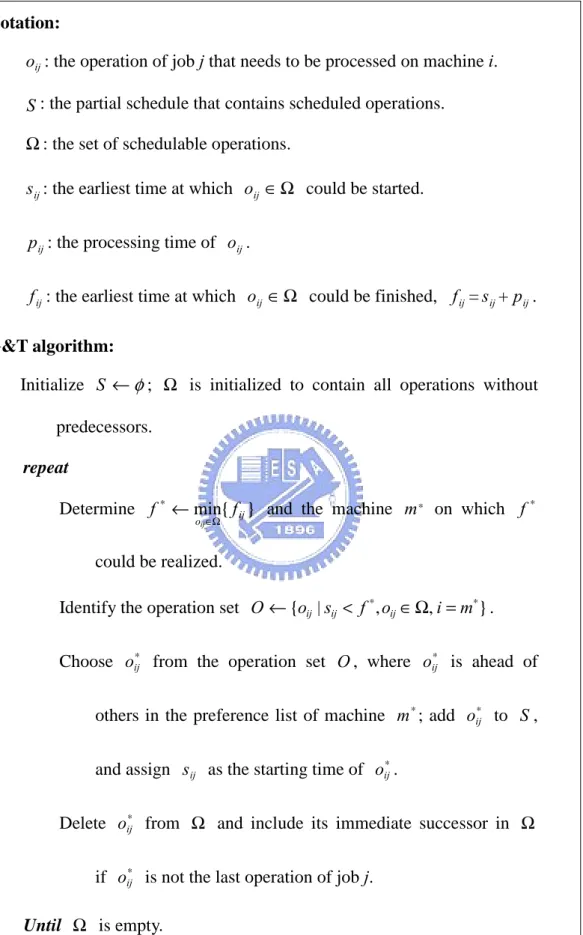
Figure 5.1 The G&T algorithm... 36

Figure 5.2 An illustration of decoding a particle position into a schedule... 37

Figure 5.3 The pseudo code of updating velocities... 45

Figure 5.4 An instance of particle movement. ... 48

Figure 5.5 Pseudo code of particle movement. ... 49

Figure 5.6 Pseudo code of updating pbest solution and gbest solution with diversification strategy. ... 51

Figure 5.7 An illustration of neighborhoods in tabu search... 53

Figure 6.1 The pseudo code of updating velocities... 70

Figure 6.2 The pseudo code of particle movement... 72

Figure 6.3 The G&T algorithm for OSSP. ... 74

Figure 6.4 Parameterized active schedules. ... 76

(10)

LIST OF TABLES

Table 2.1 References of PSO for discrete optimization problems... 6

Table 4.1 Computational results ... 30

Table 4.2 The percentage gaps between DPSO+LS and Fix+LP+LS (Vasquez and Vimont, 2005) ... 31

Table 4.3 Summary of the DPSO for MKP ... 32

Table 5.1 A 4×4 job shop problem example ... 35

Table 5.2 Computational result of FT and LA test problems... 57

Table 5.3 Computation time of FT and LA test problems (in CPU seconds). ... 59

Table 5.4 Computational result of TA test problems. ... 60

Table 5.5 Comparison with TSSB (Pezzella & Merelli, 2000) on TA test problems. ... 62

Table 5.6 Summary of the HPSO for JSSP... 63

Table 6.1(a) Computational results of four decoding operators with mutation operator... 84

Table 6.2 Results of the test problems proposed by Taillard (1993)... 87

Table 6.3 Results of the test problems proposed by Brucker et al. (1997) ... 89

Table 6.4 Results of the test problems proposed by Guéret and Prins (1999) ... 91

(11)

CHAPTER 1 INTRODUCTION

1.1 Research Motivations

In an optimization problem, limited resources need to be allocated for maximum

profit. When an optimization problem has discrete solution space, solving such a

problem amounts to making discrete choice such that an optimal solution is found

among a finite or a countable infinite number of alternatives. Such problems are

called discrete optimization problems. Typically, the task is complex, limiting the

practical utility of combinatorial, mathematical programming and other analytical

methods in solving discrete optimization problems effectively.

To find exact solutions of discrete optimization problems a branch-and-bound or

dynamic programming algorithm is often used. However, many discrete optimization

problems are NP-hard, which means that the problem cannot be exactly solved in a

reasonable computation time. Using problem-specific information sometimes reduces

search space, even though the problem is still difficult to solve exactly. Therefore,

heuristic algorithms are developed to obtain the approximate optimal solution.

Metaheuristic is one of the most popular and the most efficient method to obtain the

approximate optimal solution. Among the meta-heuristics, particle swarm

optimization (PSO) is new and extensively implemented in recent years. However, the

original intent of PSO is to solve continuous optimization problems, and PSO

methods that work well for discrete optimization problems are still scarce.

1.2 Research Objectives

(12)

optimization problems: the multidimensional 0-1 knapsack problem (MKP), the job

shop scheduling problem (JSSP) and the open shop scheduling problem (OSSP).

Since the original intent of PSO is to solve continuous optimization problems,

we have to modify the original PSO when we implement PSO to a discrete

optimization problem. PSO can be separated several parts to discuss: position

representation, particle velocity, and particle movement. We will develop various PSO

designs in this work. On the other hand, the PSO developed in this work can be an

example of PSO design for other discrete optimization problems.

1.3 Organization

The organization of the remaining chapters for this research is as follows.

Chapter 2 reviews the literatures of the background of the multidimensional 0-1

knapsack problem, shop scheduling problems and PSO. Chapter 3 infers the possibly

success factors of PSO design. Chapter 4 shows a PSO for MKP, chapter 5 shows a

PSO for JSSP, and chapter 6 shows a PSO for OSSP. In chapter 7 we draw our

(13)

CHAPTER 2 LITERATURE REVIEW

2.1 Particle Swarm Optimization

Particle swarm optimization (PSO) was developed by Kennedy and Eberhart

(1995). The original intention was to simulate the movement of organisms in a bird

flock or fish school, and it has since been introduced as an optimization technique.

PSO is a population-based optimization algorithm. Each particle is an individual, and

the swarm is composed of particles. The relationship between swarm and particles in

PSO is similar to the relationship between population and chromosomes in genetic

algorithm (GA).

In PSO, the problem solution space is formulated as a search space. Each

position in the search space is a correlated solution of the problem. For example,

when PSO is applied to a continuous optimization problem with d variables, the

solution space can be formulated as a d dimensional search space, and the value of jth variable is formulated as the position on jth dimension. Particles cooperate to find the best position (best solution) in the search space (solution space). The particle

movement is mainly affected by three factors: inertia, particle best position (pbest),

and global best position (gbest). The inertia is the velocity of the particle in the latest

iteration, and it can be controlled by inertia weight. The intention of the inertia is to

prevent particles from moving back to their current positions. The pbest position is the

best solution found by each particle itself so far, and each particle has its own pbest

position. The gbest position is the best solution found by the whole swarm so far.

Each particle moves according to its velocity. The velocity is randomly generated

(14)

position of particles can be updated by the following equations: ) ( ) ( ₂ ₂ 1 1 kj kj j kj kj

kj w v c rand pbest x c rand gbest x

v ← × + × × − + × × − (2.1)

kj kj

kj x v

x ← + (2.2)

In equation (2.1) and equation (2.2), v is the velocity of particle k on _kj

dimension j, which value is limited to the parameter Vmax, that is, vkj ≤Vmax. The

kj

x is the position of particle k on dimension j, which value is limited to the

parameter X_max, that is, x_kj ≤ X_max. Thepbest is the pbest position of particle k _kj on dimension j, and gbest is the gbest position of the swarm on dimension j. The _j inertia weight w was first proposed by Shi and Eberhart (1998a, 1998b), and it is used to control exploration and exploitation. The particles maintain high velocities

with a larger w, and low velocities with a smaller w. A larger w can prevent particles from becoming trapped in local optima, and a smaller w encourages particles exploiting the same search space area. The constants c1 and c2 are used to

decide whether particles prefer moving toward a pbest position or gbest position. The

1

rand and rand2 are random variables between 0 and 1. The process of PSO is

(15)

Initialize a population of particles with random positions and velocities on

d dimensions in the search space.

repeat

for each particle k do

Update the velocity of particle k, according to equation (1). Update the position of particle k, according to equation (2). Map the position of particle k in the solution space and evaluate its fitness value according to the desired optimization fitness function.

Update pbest and gbest position if necessary.

end for

until a criterion is not met, usually a sufficient good fitness or a maximum

number of iterations.

Figure 2.1 The process of particle swarm optimization.

The original PSO is suited to a continuous solution space. Therefore, the

applications of PSO for discrete optimization problems are still scarce. Table 2.1

(16)

Table 2.1 References of PSO for discrete optimization problems

Problem References

Binary Unconstrained Optimization Kennedy & Eberhart (1997)

A first discrete version of PSO for binary variables.

Rastegar et al. (2004)

Based on Kennedy & Eberhart (1997), hybridized with learning automata.

Constrained layout optimization Li (2004)

Represent a layout problem by continuous variables.

Multi-objective task allocation Yin et al. (2007a)

Particle represented by integer variables, which indicates the index of the allocated processor for each module.

Task assignment problem Salman et al. (2002)

The positions of tasks are represented by continuous variables.

Yin et al. (2007b)

Hybridized with a parameter-wise hill-climbing heuristic.

Traveling salesman problem Wang et al. (2003)

Applied sequential ordering representation and swap operator. Pang et al. (2004)

Represent the particle position by a fuzzy matrix.

Zhi et al. (2004)

The particles movement is based on a one-point crossover.

Vehicle routing problem Wu et al. (2004)

Applied swap operator and 2-opt local search.

(17)

Table 2.1 (cont.)

Problem References

Scheduling Problems:

– Assembly scheduling Allahverdi & Al-Anzi (2006) Hybridized with tabu search.

– Flow shop scheduling Lian et al. (2006)

Proposed three crossover operators. Tasgetiren et al. (2007)

Real number representation and local search.

Liao et al. (2007)

Represent the operation sequence by 0-1 variables.

– Job shop scheduling Lian et al. (2006)

Proposed four crossover operators.

– Multi-objective flexible job-shop scheduling

Xia & Wu (2005)

Hybridized with simulated annealing.

– Resource constraint project scheduling

Zhang & Li (2006) Zhang & Li (2007)

Compared priority based representation and sequential ordering representation.

(18)

2.2 Multidimensional 0-1 Knapsack Problem

The multidimensional 0-1 knapsack problem (MKP) is a well-known NP-hard

problem. The problem can be formulated as:

maximize

∑

= n j j jx p 1 , subject to

∑

= ≤ n j i j ijx b r 1 , for i=1,_K,m, } 1 , 0 { ∈ j x , for j=1,_K,n, with pj >0, for all j,

i ij b r ≤ ≤ 0 , for all i, j,

∑

= < n j ij i r b 1 , for all i.

Where m is the number of knapsack constraints and n is the number of items. Each item j requires rij units of resource consumption in the ith knapsack and yields

j

p units of profit upon inclusion. The goal is to find a subset of items that yields maximum profit without exceeding resource capacities. The MKP can be seen as a

general model for any kind of binary problems with positive coefficients, and it can be

applied to many problems such as cargo loading, capital budgeting, project selection,

etc. The most recent surveys on MKP can be found in (Fréville, 2004) and (Fréville

and Hanafi, 2005).

The MKP is an NP-hard problem, so it cannot be exactly solved in a reasonable

computation time for large instances. However, metaheuristics can obtain approximate

optimal solutions in a reasonable computation time. For that reason, metaheuristics for

MKP such as simulated annealing (SA) (Drexl, 1988), tabu search (TS) (Glover and

Kochenberger, 1996; Hanafi and Fréville; 1998; Vasquez and Hao, 2001; Vasquez and

(19)

during the last decade.

2.3 Job Shop Scheduling Problem

The job shop scheduling problem (JSSP) is one of the most difficult

combinatorial optimization problems. The JSSP can be briefly stated as follows

(French, 1982; Gen & Cheng, 1997). There are n jobs to be processed through m machines. We shall suppose that each job must pass through each machine once and

once only. Each job should be processed through the machines in a particular order,

and there are no precedence constraints among different job operations. Each machine

can process only one job at a time, and it cannot be interrupted. Furthermore, the

processing time is fixed and known. In this work, the problem is to find a schedule to minimize the makespan (C_max), that is, the time required to complete all jobs. The constraints in the classical JSSP is listed as follows (Bagchi, 1999):

• No two operations of one job occur simultaneously.

• No pre-emption (i.e. process interruption) of an operation is allowed.

• No job is processed twice on the same machine.

• Each job is processed to its completion, though there may be waits and

delays between the operations performed.

• Jobs may be started at any time; hence no release time exists.

• Jobs must wait for the next machine to be available.

• No machine may perform more than one operation at a time.

• Set-up times for the operations are sequence-independent and included

in processing times.

• There is only one of each type of machine.

• Machines may be idle within the schedulable period.

(20)

• The technological (usually related to processing) constraints are known

in advance and are immutable.

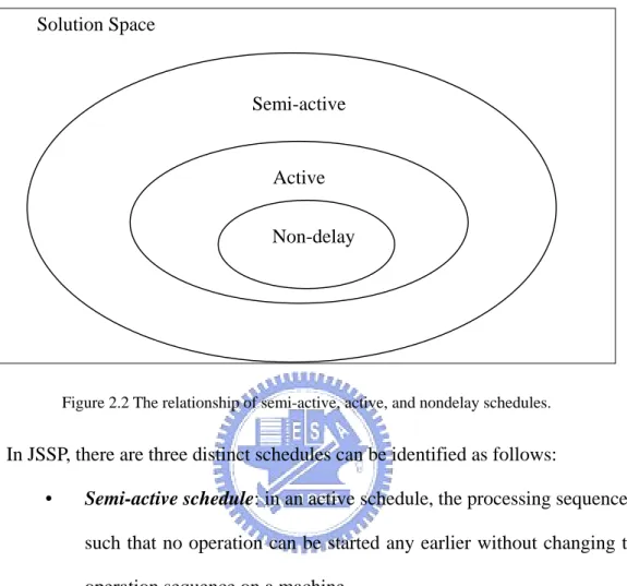
Solution Space

Semi-active

Active

Non-delay

Figure 2.2 The relationship of semi-active, active, and nondelay schedules. In JSSP, there are three distinct schedules can be identified as follows:

• Semi-active schedule: in an active schedule, the processing sequence is

such that no operation can be started any earlier without changing the

operation sequence on a machine.

• Active schedule: in an active schedule, the processing sequence is such

that no operation can be started any earlier without delaying some

other operation.

• Nondelay schedule: in a nondelay schedule, no machine is kept idle at

a time when it could begin processing other operations.

Figure 2.2 shows the relationship of semi-active, active, and nondelay schedules. The

optimal JSSP solution should be an active schedule. To reduce the search solution

space, the tabu search proposed by Sun et al. (1995) searches solutions within the set

(21)

parameterized active schedules. The main purpose of parameterized active schedules

is to reduce the search area but not to exclude the optimal solution. The basic idea of

parameterized active schedules is to control the search area by controlling the delay

times that each operation is allowed. If all of the delay times are equal to zero, the set

of parameterized active schedules is equivalent to non-delay schedules. On the

contrary, if all of the delay times are equal to infinity, the set of parameterized active

schedules is equivalent to the active schedules.

Garey et al. (1976) demonstrated that JSSP is NP-hard, so it cannot be exactly

solved in a reasonable computation time. Many meta-heuristics have been developed

in the last decade to solve JSSP, such as simulated annealing (SA) (Lourenço, 1995),

tabu search (TS) (Sun et al., 1995; Nowicki & Smutnicki, 1996; Pezzella & Merelli, 2000), and genetic algorithm (GA) (Bean, 1994; Kobayashi et al., 1995; Wang & Zheng, 2001; Gonçalves et al., 2005).

2.4 Open Shop Scheduling Problem

The open shop scheduling problem (OSSP) can be stated as follows (Gonzalez &

Sahni, 1976): there is a set of n jobs that have to be processed on a set of m machines. Every job consists of m operations, each of which must be processed on a different machine for a given process time. The operations of each job can be processed in any

order. At any time, at most one operation can be processed on each machine, and at

most one operation of each job can be processed. In this research, the problem is to

find a non pre-emptive schedule to minimize the makespan (Cmax), that is, the time

required to complete all jobs.

The constraints in the classical OSSP are similar to the classical JSSP but there

(22)

for m≥3 (Gonzalez & Sahni, 1976), so it cannot be exactly solved in a reasonable computation time. Guéret and Prins (1998) proposed two fast heuristics, the results of which are better than other classical heuristics. Domdorf et al. (2001) proposed a branch-and-bound method, which is the current best method to solve OSSP exactly. Many metaheuristic algorithms have been developed in the last decade to solve OSSP, such as simulated annealing (SA) (Liaw, 1999), tabu search (TS) (Alcaide & Sicilia, 1997; Liaw, 1999), genetic algorithm (GA) (Liaw, 2000; Prins, 2000), ant colony

optimization (ACO) (Blum, 2005), and neural network (NN) (Colak & Agarwal,

(23)

CHAPTER 3 DEVELOPING A PARTICLE SWARM OPTIMIZATION

FOR A DISCRETE OPTIMIZATION PROBLEM

The original PSO is suited to a continuous solution space. We have to modify the original PSO in order to better suit it to discrete optimization problems. In this chapter, we will discuss the probably success factors to develop a PSO design for a discrete optimization problem. We separated a PSO design into several parts to discuss: particle position representation, particle velocity, particle movement, decoding operator, and other search strategies.

3.1 Particle Position Representation

PSO represents the solutions by particle positions. There are various particle position representations for a discrete optimization problem. How to represent solutions by particle positions is a research topic when we develop a PSO design.

Generally, the Lamarckian property is used to discriminate between good and bad representations. The Lamarckian property is that the offspring can inherit goodness from its parents. For example, if there are six operations to be sorted on a machine, and we implement the random key representation (Bean, 1994) to represent a sequence, there are two positions of two particle positions as follows:

position 1: [0.25, 0.27, 0.21, 0.24, 0.26, 0.23]

position 2: [0.22, 0.25, 0.23, 0.26, 0.24, 0.21]

Then the operation sequence can be generated by sort the operations according to the increasing order of their position values as follows:

(24)

permutation 1: [3 6 4 1 5 2]

permutation 2: [6 1 3 5 2 4]

We can find that these two permutations are quite different even though their positions are very close to each other. This is because the location in the permutation of one operation depends on the position values of other operations. Hence, the random key representation has no Lamarckian.

If we directly implement the original PSO design (i.e. the particles search solutions in a continuous solution space) to a scheduling problem, we can implement the random key representation to represent a sequence of operations on a machine. However, the PSO will be more efficient if the particle position representation is with higher Lamarckian.

3.2 Particle Velocity and Particle Movement

The particle velocity and particle movement are designed for the specific particle position representation. In each iteration, a particle moves toward pbest and gbest positions, that is, the next particle position is determined by current position, pbest position, and gbest position. Furthermore, particle moves according to its velocity and movement mechanisms. Each particle moves from current position (solution) to one of the neighborhood positions (solutions). Therefore, the particle movement mechanism should be designed according the neighborhood structure. The advantage of neighborhood designs can be estimated by following properties (Mattfeld, 1996):

• Correlation: the solution resulting from a move should not differ much

from the starting one.

• Feasibility: the feasibility of a solution should be preserved by all

(25)

• Improvement: all moves in the neighborhood should have a good

chance to improve the objective of a solution.

• Size: the number of moves in the neighborhood should be reasonably

small to avoid excessive computational cost of their evaluation.

• Connectivity: it should be possible to reach the optimal solution from

any starting one by performing a finite number of neighborhood moves.

We believe that the PSO will be more efficient if we design the particle velocity and the particle movement mechanisms according to these properties.

3.3 Decoding Operator

Decoding operator is used to decode a particle position into a solution. The decoding operator is designed according the specific particle position representation and the characteristics of the problem. A superior decoding operator can map the positions to the solution space in a smaller region but not excluding the optimal solution. In chapter 6, we designed four decoding operators for OSSP. The results show that the decoding operator design extremely influences the solution quality.

3.4 Other Search Strategies

．Diversification Strategy

We can also consider implementing other search strategies. The purpose of most search strategies is to control the intensification and the diversification. One of the search strategies is the structure of gbest and pbest solutions. In the original PSO design, each particle has its own pbest solution and the swam has only one gbest solution. Eberhart and Shi (2001) show a “local” version of the particle swarm. In this version, particles have information only of their own and their neighbors’ bests, rather

(26)

that that of the entire group. Instead of moving toward a kind of stochastic average of

pbest and gbest (the best location of the entire group), particles move toward points

defined by pbest and “lbest,” which is the index of the particle with the best evaluation in the particle’s neighborhood.

In this research, we proposed a diversification strategy. In this strategy, the pbest solution of each particle is not the best solution found by the particle itself, but one of the best N solutions found by the swarm so far where N is the size of the swarm.

．Selection Strategy

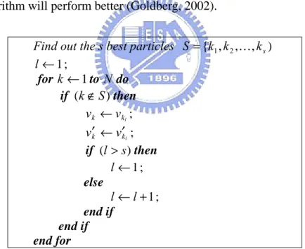
Angeline (1998) proposed a selection strategy, which is performed as follows. After all the particles move to new positions, select the s best particles. The better particle set S ={k₁,k₂,_K,k_s) replaces the positions and velocities of the other particles. The addition of this selection strategy should provide the swarm with a more exploitative search mechanism that should find better optima more consistently.

In chapter 4, we modified the method proposed by Angeline (1998) based on the concept of building blocks where a block is part of a solution, and a good solution should include some superior blocks. The concept of building blocks is that if we can precisely find out the superior blocks and accumulate the superior blocks in the population, the genetic algorithm will perform better (Goldberg, 2002).

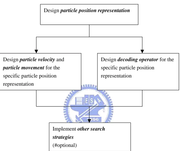
3.5 The Process to Develop a New Particle Swarm Optimization

As mentioned above, we separated PSO into several parts. The particle position representation determines the program data structure and other parts are designed for the specific particle position representation. Therefore, the first step of developing a new PSO is to determine the particle position representation. Then design particle

(27)

representation. Finally implement some search strategies for further improving solution quality. Figure 3.1 shows the process to develop a new particle swarm optimization. All the PSOs in this research are developed by the process described as Figure 3.1.

Figure 3.1 The process to develop a new particle swarm optimization

Design particle position representation

Design particle velocity and

particle movement for the specific particle position representation

Design decoding operator for the specific particle position

representation

Implement other search

strategies

(28)

CHAPTER 4 A DISCRETE BINARY PARTICLE SWARM

OPTIMIZATION FOR THE MULTIDIMENSIONAL 0-1

KNAPSACK PROBLEM

Kennedy and Eberhart (1997) proposed a discrete binary particle swarm optimization (DPSO), which was designed for discrete binary solution space. Rastegar et al. (2004) proposed another DPSO based on learning automata. In both of the DPSOs, when particle k moves, its position on the jth variable x equals 0 or 1 at _kj

random. The probability that x equals 1 is obtained by applying a sigmoid _kj

transformation to the velocity v ))_kj (1/1+exp(−v_kj . In the above two DPSOs, the positions and velocities of particles can be updated by the following equations:

) ( ) ( 2 2 1 1 kj kj j kj kj

kj v c rand pbest x c rand gbest x

v ← + × × − + × × − (4.1) 0 1 )) exp( 1 / 1 (

(rand < + −v_kj thenx_kj ← elsex_kj ←

if (4.2)

where rand, rand , and 1 rand are random numbers between 0 and 1. The 2

value of v is limited by a value _kj Vmax, a parameter of the algorithm, that is, max

|

|v_kj ≤V . For instance, if Vmax= 6, the probability that x equals 1 will be limited kj

between 0.9975 and 0.0025.

The DPSOs proposed by Kennedy and Eberhart (1997) and Rastegar et al. (2004) are designed for discrete binary optimization problems with no constraint. However, there are resource constraints in MKP. If we want to solve MKP by DPSO, we have to modify DPSO to fit the MKP characteristics.

(29)

in previous research: (i) particle velocity and (ii) particle movement. The particle velocity is modified based on the tabu list and the concept of building blocks, and then the particle movement is modified based on the crossover and mutation of the genetic algorithm (GA). Besides, we applied the repair operator to repair solution infeasibility, the diversification strategy to prevent particles becoming trapped in local optima, the selection strategy to exchange good blocks between particles, and the local search to further improve solution quality. The computational results show that our DPSO effectively solves MKP and better than other traditional algorithms.

4.1 Particle Position Representation

In out DPSO, the particle position is represented by binary variables. For a MKP with n items, we represent the particle k position by n binary variables, i.e.

] , , , [ k1 k2 kn k x x x x = _K

Where x_kj∈

{ }

0,1 denotes the value of jth variable of particle k’s solution. Each time we start a run, DPSO initializes a population of particles with random positions, and initializes the gbest solution by a surrogate duality approach (Pirkul, 1987). We

determine the pseudo-utility ratio

∑

=

= j m_i i ij

j p yr

u

1

/ for each variable, where yi is

the shadow price of the ith constraint in the LP relaxation of the MKP. To initialize the

gbest solution, we set gbestj ←0 for all variable j and then add variables

(gbest_j ←1) into the gbest solution by descending order of u_j as much as possible without violating any constraint.

Initializing the gbest solution has two purposes. The first is to improve the consistency of run results. Because the solutions of DPSO are generated randomly, the computational results will be different in each run. If we give DPSO the same initial point of gbest solution in each run, it may improve result consistency. The second

(30)

purpose is to improve result quality. Similar to other local search approaches, a good initial solution can accelerate solution convergence with better results.

4.2 Particle Velocity

When PSO is applied to solve problems in a continuous solution space, due to inertia, the velocity calculated by equation (4.1) not only moves the particle to a better position, but also prevents the particle from moving back to the previous position. The larger the inertia weight, the harder the particle backs to the current position. The DPSO velocities proposed by Kennedy and Eberhart (1997) and Rastegar et al. (2004) move particles toward the better position, but cannot prevent the particles from being trapped in local optima.

We modified the particle velocity based on the tabu list, which is applied to prevent the solution from being trapped in local optima. In our DPSO, each particle has its own tabu list, the velocity. There are two velocity values, v and kj vkj′ , for

each variable x . If _kj x changes when particle k moves, we set _kj v_kj←1 and v_kj′ ← kj

x . When v equals 1, it means that kj x has changed, variable j was added into the kj

tabu list of particle k, and we should not change the value of x in the next few _kj iterations. Therefore, the velocity can prevent particles from moving back to the last position in the next few iterations. The value of v_kj′ is used to record the value of x _kj after the value of x has been changed. The set of variable kj vkj′ is a “block” which

is a part of a solution that particle k obtained from the pbest solution and gbest solution. It is applied to the selection strategy with the concept of building blocks that we will describe in section 4.6.

In our DPSO, we also implement inertia weight w to control particle velocities where w is between 0 and 1. We randomly update velocities at the beginning of each

(31)

iteration. For each particle k and jth variable, if v equals 1, _kj v will be set to 0 with _kj probability (1- w ). This means that if variable x is in the tabu list of particle k, kj

variable x will be dropped from the tabu list with probability (1- w ). Moreover, the _kj exploration and exploitation can be controlled by w . The variable x will be held kj

in the tabu list for more iterations with a larger w and vice versa. The pseudo code of updating velocities is given in Figure 4.1.

for each particle k and variable j do

rand ~ U(0,1)

if (vkj =1)and (rand ≥w) then 0 ← kj v end if end for

Figure 4.1 Pseudo code of updating velocities.

4.3 Particle Movement

In the DPSO we proposed, particle movement is similar to the crossover and mutation of GA. When particle k moves, if x is not in the tabu list of particle k (i.e. kj

kj

v =0), the value of x will be set to kj pbest with probability kj c (if 1

kj

x ≠ pbest ), set to kj gbest with probability j c (if 2 xkj ≠ gbest ), set to (1-j x ) kj with probability c , or not changed with probability (1-3 c -1 c -2 c ). Where 3 c , 1 c , 2 and c are parameters of the algorithm with ₃ c1+c2 +c3 ≤1 and ci ≥0, i=1, 2, 3.

Since the value of x may be changed by repair operator or local search kj

procedure (we will describe them in section 4.4 and in section 4.7 respectively), if x _kj is in the tabu list of particle k (i.e. v = 1), the value of kj x will be set to the value of kj

kj

v′ which is the latest value that x obtained from the pbest solution or gbest kj

solution. At the same time, if the value of x changes, we update kj v and kj vkj′ as

(32)

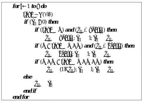
4.2. for j←1 to n do rand ~ U(0,1) then if (v_kj =0) then and if (rand≤c1) (xkj ≠ pbestkj) kj kj kj kj kj pbest v v x x ← ; ←1; ′ ← then and if (c1 <rand ≤c1+c2) (xkj ≠gbestj) kj kj kj j kj gbest v v x x ← ; ←1; ′ ← then if (c1+c2 <rand ≤c1+c2 +c3) kj kj kj kj kj x v v x x ←(1− ); ←1; ′ ← else kj kj v x ← ′ end if end for

Figure 4.2 Pseudo code of particle movement.

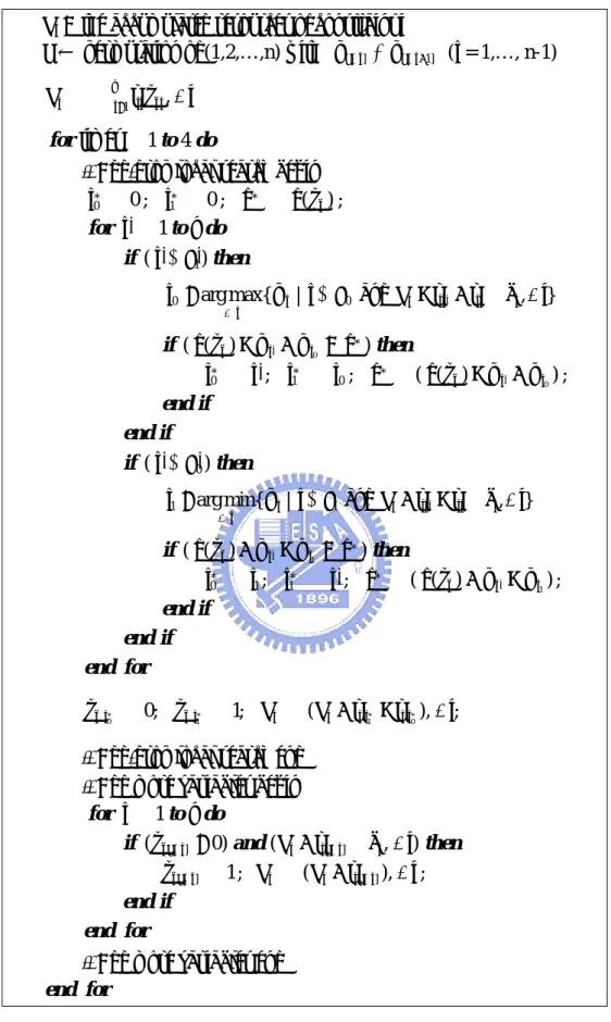
4.4 Repair Operator

After a particle generates a new solution, we apply the repair operator to repair solution infeasibility and to improve it. There are two phases to the repair operator. The first is the drop phase. If the particle generates an infeasible solution, we need to drop (xkj ←0, if xkj =1) some variables to make it feasible. The second phase is the

add phase. If the particle finds a feasible solution, we add (x_kj ←1, if x_kj =0) more variables to improve it. Each phase is performed twice: the first time we consider the particle velocities, and the second time we do not consider the particle velocities.

Similar to initializing the gbest solution described in section 4.1, we applied the Pirkul (1987) surrogate duality approach to determine the variable priority for adding

or dropping. First, we determine the pseudo-utility ratio

∑

= = j m_i i ij j p yr u 1 / for each

variable, where y is the shadow price of the i_i th constraint in the LP relaxation of the MKP. We drop variables by ascending order of u until the solution is feasible, and j

(33)

violating any constraint. The pseudo code of repair operator is given in Figure 4.3.

Ri = the accumulated resources of constraint i

U

←

permutation of (1,2,…,n) with uU[j]≥uU[j+1] (j = 1,…, n-1)

∑

= ∀ ← n_j ij kj i r x i R ₁ , ; begin phase Drop // do to for j←n 1 then and and if (xkU[j] =1) (Ri >bi, foranyi) (vkU[j]=0) ; 0 ] [j ← kU x ; ), (R r [ ] i R_i ← _i − _iU _j ∀ if end for end do to for j←n 1 then and and if (xkU[j] =1) (Ri >bi, foranyi) (vkU[j]=1) ; 0 ] [j ← kU x ; ), (R r [ ] i R_i ← _i − _iU _j ∀ if end for end end phase Drop // begin phase Add // do to for j←1 n then and and if (xkU[j] =0) (Ri +riU[j]≤bi,∀i) (vkU[j]=0) 1 ] [j ← kU x ; i r R R_i ←( _i + _iU[_j]),∀ ; if end for end do to for j←1 n then and and if (xkU[j] =0) (Ri +riU[j]≤bi,∀i) (vkU[j]=1) 1 ] [j ← kU x ; i r R R_i ←( _i + _iU[_j]),∀ ; if end for end end phase Add //

(34)

4.5 The Diversification Strategy

If the pbest solutions are all the same, the particles will be trapped in local optima. To prevent such a situation, we propose a diversification strategy to keep the

pbest solutions different. In the diversification strategy, the pbest solution of each

particle is not the best solution found by the particle itself, but one of the best N solutions found by the swarm so far where N is the size of the swarm.

The diversification strategy is performed according to the following process. After all of the particles generate new solutions, for each particle, compare the particle’s fitness value with pbest solutions. If the particle’s fitness value is better than the worst pbest solution and the particle’s solution is not equal to any of the pbest solutions, replace the worst pbest solution with the solution of the particle. At the same time, if the particle’s fitness value is better than the fitness value of the gbest solution, replace the gbest solution with the solution of the particle. The pseudo code of updating pbest solutions is given in Figure 4.4.

*

k is the index of the worst pbest solution

for k ← 1 to N do

{

( )

}

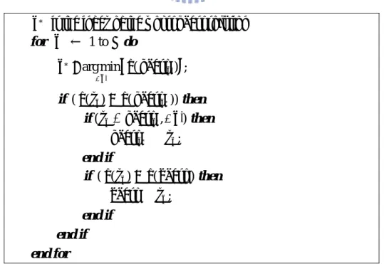
min arg * k k pbest f k _′ ′ ∀ = ; then if (f(x_k)> f(pbest_k*)) then if(x_k ≠ pbest_k',∀k′) k k x pbest * ← ; end if then if (f(xk)> f(gbest)) k x gbest← ; end if end if end for

(35)

4.6 The Selection Strategy

Angeline (1998) proposed a selection strategy, which is performed as follows. After all the particles move to new positions, select the s best particles. The better particle set S ={k₁,k₂,_K,k_s) replaces the positions and velocities of the other particles. The addition of this selection strategy should provide the swarm with a more exploitative search mechanism that should find better optima more consistently.

We modified the method proposed by Angeline (1998) based on the concept of building blocks where a block is part of a solution, and a good solution should include some superior blocks. The concept of building blocks is that if we can precisely find out the superior blocks and accumulate the superior blocks in the population, the genetic algorithm will perform better (Goldberg, 2002).

Find out the s best particles S ={k1,k2,K,ks) 1 ← l ; do to for k←1 N then if (k∉S) l k k v v ← ; l k k v v′ ← ′ ; then if (l>s) 1 ← l ; else 1 + ← l l ; end if end if end for

Figure 4.5 Pseudo code of selection strategy.

In our DPSO, the velocities v′k ={v′k1,vk′2,K,v′kn} is a block that particle k obtained from pbest solution and gbest solution in each iteration. The v_k′ may be a superior block if the solution of particle k is better then others. Therefore, in our modified selection strategy, the better particle set S only replaces the velocities (i.e.

(36)

k

v and vk′ ) of the other particles. The pseudo code of selection strategy is given in

Figure 4.5.

4.7 Local Search

We implement a local search procedure after a particle generates a new solution for further improved solution quality. The classical add/drop neighborhood is that we remove a variable from the current solution and add another variable to it without violating any constraint at the same time. We modified the neighborhood with the concept of building blocks to reduce the neighborhood size. We focus on the block when we implement a local search. The variables are classified to 4 sets:

} 0 | { 0 = j xkj = J , }J1 ={j|xkj =1 , }J0′ ={j|xkj =0∧vkj =1 , and J1′ ={j|xkj =1 } 1 =

∧vkj . The modified neighborhood is defined as follows: add (or drop) one

variable from J0′ (or J1′) and drop (or add) one variable from J (or 1 J ) without 0 violating any constraint at the same time. In our experiment, the size of the modified neighborhood is about twenty times smaller then the classical one. Besides, we add

variables by descending order of p as much as possible without violating any _j

(37)

Ri = the accumulated resources of constraint i P

←

permutation of (1,2,…,n) with pP[j]≥ pP[j+1] (j = 1,…, n-1)

∑

= ∀ ← n_j ij kj i r x i R ₁ , do to fortimes←1 4

// Add/drop local search begin

0 * 0 ← j ; 0* 1 ← j ; )* ( k x f f ← ; do to for j′←1 n then if (j′∈J1′) } , | { max arg 0 0 p j J and R r r b i j j i ij ij i j ∈ − + ≤ ∀ = ′ ∀ then if ( ( ) *) 0 f p p x f _k − _j′+ _j > j j* ← ′ 0 ; j1* ← ; )j0 ( ( ) 0 * j j k p p x f f ← − ′+ ; if end if end then if (j′∈J0′) } , | { min arg 1 1 p j J and R r r b i j j i ij ij i j ∈ + − ≤ ∀ = ′ ∀ then if ( ( ) *) 1 f p p x f _k + _j′− _j > 1 * 0 j j ← ; j* ← j′ 1 ; )( ( ) 1 * j j k p p x f f ← + ′− ; if end if end for end ; 0 * 0 ← j k x * 1; 1 ← j k x ( *), ; 0 * 1 r i r R R_i ← _i + _i_j − _i_j ∀

// Add/drop local search end // Add more variables begin

do to for j←1 n then and if (xkP[j] =0) (Ri +riP[j] ≤bi,∀i) 1 ] [j ← kP x ; R_i ←(R_i +r_iP[_j]),∀i; if end for end

// Add more variables end

for end

(38)

We do not repeat the local search until the solution reaches the local optima. The local search procedure is performed four times at most for reducing the computation time and preventing being trapped in local optima. The pseudo code of local search is given in Figure 4.6.

4.8 Computational Results

Our DPSO was tested on the problems proposed by Chu and Beasley (1998). These problems are available on the OR-Library web site (Beasley, 1990) (URL: http:// people.brunel.ac.uk/~mastjjb/jeb/info.html). The number of constraints m was set to 5, 10, and 30, and the number of variables n was set to 100, 250, and 500. For

each m-n combination, thirty problems are generated, and the tightness ratio α

(

∑

= =bi/ n_j 1rij

α

) was set to 0.25 for the first ten problems, to 0.5 for the next ten

problems, and to 0.75 for the remaining problems. Therefore, there are 27 problem

sets for different n-m-

α

combinations, ten problems for each problem set, and 270

problems in total.

The program was coded in Visual C++, optimized by speed, and run on an AMD

Athlon 1800+ PC. The numeric parameters are set to c1 =0.7, 1c2 =0. , c3 =1/n,

N = 100, and s = 20. The inertia weight w is decreased linearly from 0.7 to 0.5

during a run. Allof the numeric parameters are determined empirically.There are two versions of our DPSO. The first version, DPSO, does not implement the local search procedure, and the second, DPSO+LS, implements the local search procedure. Each run will be terminated after 10,000 iterations on DPSO and 15,000 iterations on DPSO+LS, respectively.

(39)

according to the 10 problems of the problem set. The term ‘Average’ is applied to the average solution of 10 runs of each problem and averaged according to the 10 problems of the problem set.

t* is the average time in seconds that the DPSO or DPSO+LS takes to first reach the final best solution in a run, and T is the total time in seconds that the DPSO or DPSO+LS takes before termination in a run. The surrogate duality was pre-calculated by MATLAB, so the computation times in Table 4.1 do not include the computation time of calculating surrogate duality. The average computation time for solving LP relaxation problems was less then 1 CPU second, so the surrogate duality calculation is not important to computation time.

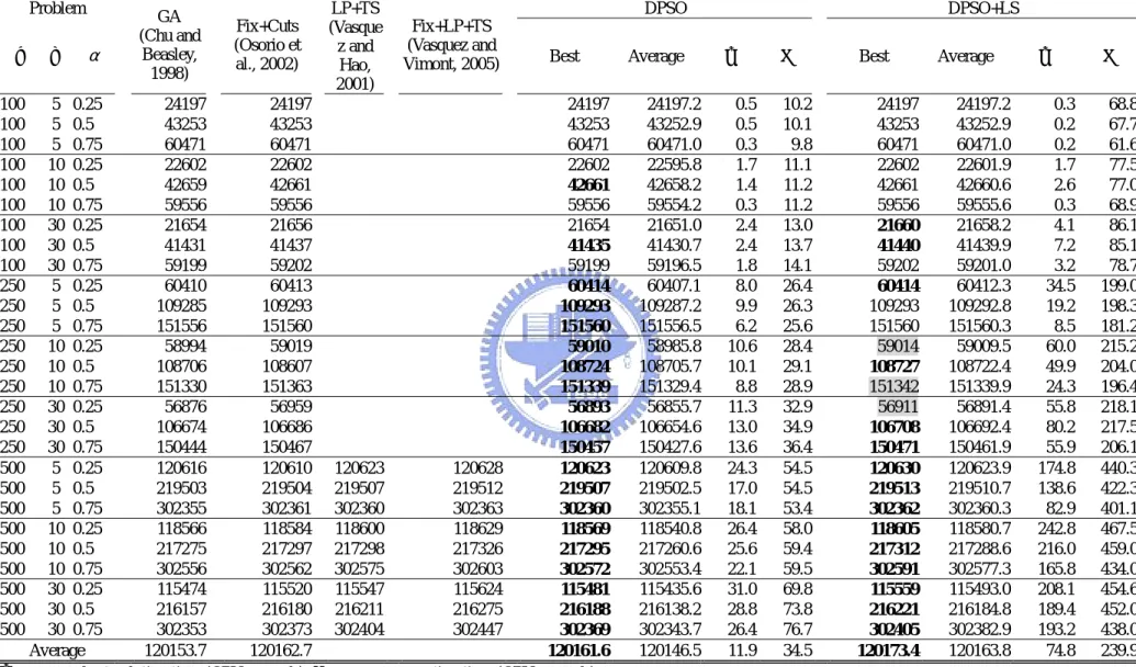
The computational results are shown in Table 4.1. The algorithms have different computation times, so we compared DPSO with GA (Chu and Beasley, 1998) since their computation times are similar. The computational results show that DPSO performed better than GA (Chu and Beasley, 1998) in 20 of 27 problem sets.

We compared DPSO+LS with Fix+Cuts (Osorio et al., 2002) and LP+TS (Vasquez and Hao, 2001). The Fix+Cuts (Osorio et al., 2002) takes 3 hours on a Pentium III 450 MHz PC for each run, and LP+TS (Vasquez and Hao, 2001) takes about 20-40 minutes on a Pentium III 500 MHz PC for each run. Our DPSO+LS takes less than 8 minutes on the largest problems and our machine is about four times faster than Fix+Cuts (Osorio et al., 2002) and LP+TS (Vasquez and Hao, 2001), so the computation time that DPSO+LS takes is similar to LP+TS (Vasquez and Hao, 2001) and much less than Fix+Cuts (Osorio et al., 2002). The computational results show that DPSO+LS performed better than Fix+Cuts (Osorio et al., 2002) in 15 of 27 problem sets, and better than LP+TS (Vasquez and Hao, 2001) in all of the 9 largest problem sets.

(40)

Table 4.1 Computational results

Problem DPSO DPSO+LS

n m α GA (Chu and Beasley, 1998) Fix+Cuts (Osorio et al., 2002) LP+TS (Vasque z and Hao, 2001) Fix+LP+TS (Vasquez and

Vimont, 2005) Best Average t

* _T Best Average t* T 100 5 0.25 24197 24197 24197 24197.2 0.5 10.2 24197 24197.2 0.3 68.8 100 5 0.5 43253 43253 43253 43252.9 0.5 10.1 43253 43252.9 0.2 67.7 100 5 0.75 60471 60471 60471 60471.0 0.3 9.8 60471 60471.0 0.2 61.6 100 10 0.25 22602 22602 22602 22595.8 1.7 11.1 22602 22601.9 1.7 77.5 100 10 0.5 42659 42661 42661 42658.2 1.4 11.2 42661 42660.6 2.6 77.0 100 10 0.75 59556 59556 59556 59554.2 0.3 11.2 59556 59555.6 0.3 68.9 100 30 0.25 21654 21656 21654 21651.0 2.4 13.0 21660 21658.2 4.1 86.1 100 30 0.5 41431 41437 41435 41430.7 2.4 13.7 41440 41439.9 7.2 85.1 100 30 0.75 59199 59202 59199 59196.5 1.8 14.1 59202 59201.0 3.2 78.7 250 5 0.25 60410 60413 60414 60407.1 8.0 26.4 60414 60412.3 34.5 199.0 250 5 0.5 109285 109293 109293 109287.2 9.9 26.3 109293 109292.8 19.2 198.3 250 5 0.75 151556 151560 151560 151556.5 6.2 25.6 151560 151560.3 8.5 181.2 250 10 0.25 58994 59019 59010 58985.8 10.6 28.4 59014 59009.5 60.0 215.2 250 10 0.5 108706 108607 108724 108705.7 10.1 29.1 108727 108722.4 49.9 204.0 250 10 0.75 151330 151363 151339 151329.4 8.8 28.9 151342 151339.9 24.3 196.4 250 30 0.25 56876 56959 56893 56855.7 11.3 32.9 56911 56891.4 55.8 218.1 250 30 0.5 106674 106686 106682 106654.6 13.0 34.9 106708 106692.4 80.2 217.5 250 30 0.75 150444 150467 150457 150427.6 13.6 36.4 150471 150461.9 55.9 206.1 500 5 0.25 120616 120610 120623 120628 120623 120609.8 24.3 54.5 120630 120623.9 174.8 440.3 500 5 0.5 219503 219504 219507 219512 219507 219502.5 17.0 54.5 219513 219510.7 138.6 422.3 500 5 0.75 302355 302361 302360 302363 302360 302355.1 18.1 53.4 302362 302360.3 82.9 401.1 500 10 0.25 118566 118584 118600 118629 118569 118540.8 26.4 58.0 118605 118580.7 242.8 467.5 500 10 0.5 217275 217297 217298 217326 217295 217260.6 25.6 59.4 217312 217288.6 216.0 459.0 500 10 0.75 302556 302562 302575 302603 302572 302553.4 22.1 59.5 302591 302577.3 165.8 434.0 500 30 0.25 115474 115520 115547 115624 115481 115435.6 31.0 69.8 115559 115493.0 208.1 454.6 500 30 0.5 216157 216180 216211 216275 216188 216138.2 28.8 73.8 216221 216184.8 189.4 452.0 500 30 0.75 302353 302373 302404 302447 302369 302343.7 26.4 76.7 302405 302382.9 193.2 438.0 Average 120153.7 120162.7 120161.6 120146.5 11.9 34.5 120173.4 120163.8 74.8 239.9 t*

(41)

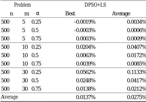
Table 4.2 The percentage gaps between DPSO+LS and Fix+LP+LS (Vasquez and Vimont, 2005) Problem DPSO+LS n m α Best Average 500 5 0.25 -0.0019% 0.0034% 500 5 0.5 -0.0003% 0.0006% 500 5 0.75 0.0003% 0.0009% 500 10 0.25 0.0204% 0.0407% 500 10 0.5 0.0063% 0.0172% 500 10 0.75 0.0039% 0.0085% 500 30 0.25 0.0562% 0.1133% 500 30 0.5 0.0248% 0.0417% 500 30 0.75 0.0138% 0.0212% Average 0.0137% 0.0275%

We do not compare our algorithms with Fix+LP+TS (Vasquez and Vimont, 2005), since Fix+LP+TS (Vasquez and Vimont, 2005) takes 7.6-33 hours on a Pentium4 2GHz PC to obtain the solution for each problem. In general, a metaheuristic does not perform such a long time and the solution quality of Fix+LP+TS (Vasquez and Vimont, 2005) could not be reached in a short computation time. However, we show the percentage gaps between our DPSO+LS and Fix+LP+TS (Vasquez and Vimont, 2005) in Table 4.2. The percentage gaps show that the results of our DPSO+LS very close to Fix+LP+TS (Vasquez and Vimont, 2005) in a short computation time.

4.9 Concluding Remarks

In this chapter we have presented a new discrete binary particle swarm optimization (DPSO) for solving multidimensional 0-1 knapsack problems and a local search procedure based on the concept of building blocks. The proposed DPSO adopted new concepts of particle velocity and particle movement, and obtained good solutions in a reasonable CPU time.

(42)

proposed DPSO can be extended for solving similar combinatorial optimization problems: for example, multidimensional 0-1 knapsack problems with generalized upper bound constraints. Second, the proposed DPSO can be extended for sequencing and scheduling problems. Similar to this chapter, we may modify the velocity based on the tabu list and the concept of building blocks, and modify particle movement based on crossover and mutation of genetic algorithm. Furthermore, we may develop the repair operator based on scheduling strategies for scheduling problems. Table 4.3 shows the summary of the DPSO for MKP.

Table 4.3 Summary of the DPSO for MKP

Components The concept of this components

1 Particle Position

Representation Binary variables

Since the solution of MKP is 0-1 variables, we represent the particle position by binary variables, which have the most Lamarckian.

Particle Velocity Blocks

2

Particle Movement Crossover operator

The binary variables is very appropriate to build blocks, so we implement the concept of building blocks and the relational crossover operator. 3 Decoding Operator Repair operator based on pseudo-utility ratio

Restrict the search area in the feasible region.

4 Other Strategies

Diversification Selection Local search

The diversification strategy can prevent particles rapped in local optima.

The selection strategy can further accelerate the speed of building blocks. The local search can further improve the solution quality,

(43)

4.10 Appendix

A pseudo code of the DPSO for MKP is given below:

Initialize a population of particles with random positions and velocities. Initialize the gbest solution by surrogate duality approach

repeat

update velocities according to Figure 4.1.

for each particle k do

move particle k according to Figure 4.2.

repair the solution of particle k according to repair operator (Figure 4.3). calculate the fitness value of particle k.

perform local search on particle k (Figure 4.6).

end for

update gbest and pbest solutions according to diversification strategy (Figure 4.4).

perform selection according to selection strategy (Figure 4.5).

(44)

CHAPTER 5 A PARTICLE SWARM OPTIMIZATION FOR THE JOB

SHOP SCHEDULING PROBLEM

The original PSO is used to solve continuous optimization problems. Since the solution space of a shop scheduling problem is discrete, we have to modify the particle position representation, particle movement, and particle velocity to better suit PSO for scheduling problems. In the PSO for JSSP, we modified the particle position representation using preference-lists and the particle movement using a swap operator. Moreover, we propose a diversification strategy and a local search procedure for better performance.

5.1 Particle Position Representation

We implement the preference list-based representation (Davis, 1985), which has half-Lamarckian (Cheng et al., 1996). In the preference list-based representation, there is a preference list for each machine. For an n-job m-machine problem, we can represent the particle k position by an m×n matrix, and the ith

row is the preference list of machine i, i.e. ⎥ ⎥ ⎥ ⎥ ⎥ ⎦ ⎤ ⎢ ⎢ ⎢ ⎢ ⎢ ⎣ ⎡ = k mn k m k m k n k k k n k k k x x x x x x x x x X L M L L 2 1 2 22 21 1 12 11 .

Where x_ijk∈

{

1,2,_K,n

}

denotes the job on location j in the preference list of machine i. Similar to GA (Kobayashi et al., 1995) decoding a chromosome into a schedule, we also use Giffler & Thompson’s heuristic (Giffler &

(45)

Thompson, 1960) to decode a particle’s position to an active schedule. The G&T algorithm is shown as Figure 5.1. For example, there are 4 jobs and 4 machines

as shown on ⎥ ⎥ ⎥ ⎥ ⎦ ⎤ ⎢ ⎢ ⎢ ⎢ ⎣ ⎡ = 2 1 4 3 1 4 3 2 4 3 1 2 3 4 2 1 k X .

Table 5.1, and the position of particle k is

⎥ ⎥ ⎥ ⎥ ⎦ ⎤ ⎢ ⎢ ⎢ ⎢ ⎣ ⎡ = 2 1 4 3 1 4 3 2 4 3 1 2 3 4 2 1 k X .

Table 5.1 A 4×4 job shop problem example

jobs machine sequence processing times

1 1, 2, 4, 3 p = 5, ₁₁ p = 4, 21 p = 2, 41 p = 2 31

2 2, 1, 3, 4 p = 4, ₂₂ p = 3, 12 p = 3, 32 p = 2 42

3 4, 1, 3, 2 p = 2, ₄₃ p = 2, 13 p = 3, 33 p = 4 23

4 3, 1, 4, 2 p = 3, ₃₄ p = 2, 14 p = 3, 44 p = 4 24

We can decode X to an active schedule following the G&T algorithm: k

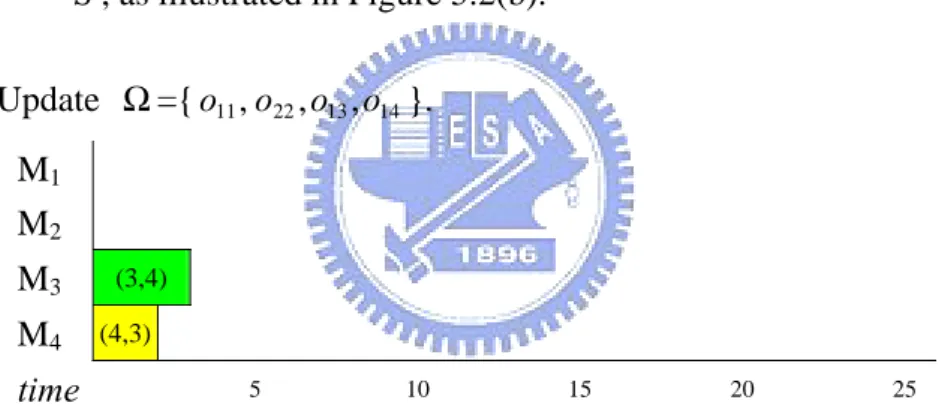
Initialization S =

_φ

; }Ω={o11,o22,o43,o34 . Iteration 1 11 s = 0, s = 0, 22 s =0, 43 s =0; 34 f = 5, 11 f = 4, 22 f = 2, 43 f = 3; 34 f = * min{ f , 11 f , 22 f , 43 f } = 2, 34 m =4. *

Identify the operation set O={o43}; choose operation o , which is ahead 43 of others in the preference list of machine 4, and add it into schedule

S , as illustrated in Figure 5.2(a).

粒子群演算法於離散最佳化問題之研究

國立交通大學

工業工程與管理學系

博士論文

粒子群演算法於離散最佳化問題之研究

A Study on Particle Swarm Optimization for

Discrete Optimization Problems

研究生 ： 徐誠佑

指導教授 ： 沙永傑 博士

陳文智 博士

中華民國九十六年五月

粒子群演算法於離散最佳化問題之研究

A Study on Particle Swarm Optimization for Discrete

Optimization Problems

研 究 生： 徐誠佑

Student： Cheng-Yu

Hsu

指導教授： 沙永傑

Advisor： Dr. David Yung-Jye Sha

陳文智

Dr. Wen-Chih Chen

國 立 交 通 大 學

工 業 工 程 與 管 理 學 系

博 士 論 文

粒子群演算法於離散最佳化問題之研究

中 文 摘 要

A Study on Particle Swarm Optimization for Discrete

Optimization Problems

ABSTRACT

誌 謝

CONTENTS

LIST OF FIGURES

LIST OF TABLES

CHAPTER 1

INTRODUCTION

1.1 Research Motivations

1.2 Research Objectives

1.3 Organization

CHAPTER 2

LITERATURE REVIEW

2.1 Particle Swarm Optimization

2.2 Multidimensional 0-1 Knapsack Problem

∑

∑

∑

2.3 Job Shop Scheduling Problem

2.4 Open Shop Scheduling Problem

CHAPTER 3

DEVELOPING A PARTICLE SWARM OPTIMIZATION

FOR A DISCRETE OPTIMIZATION PROBLEM

3.1 Particle Position Representation

3.2 Particle Velocity and Particle Movement

3.3 Decoding Operator

3.4 Other Search Strategies

3.5 The Process to Develop a New Particle Swarm Optimization

CHAPTER 4

A DISCRETE BINARY PARTICLE SWARM

OPTIMIZATION FOR THE MULTIDIMENSIONAL 0-1

KNAPSACK PROBLEM

4.1 Particle Position Representation

{ }

∑

4.2 Particle Velocity

4.3 Particle Movement

4.4 Repair Operator

∑

←

∑

4.5 The Diversification Strategy

{

}

4.6 The Selection Strategy

4.7 Local Search

←

∑

4.8 Computational Results

∑

α

α

4.9 Concluding Remarks

研究生：徐誠佑

指導教授：沙永傑博士

陳文智博士

研究生：徐誠佑

指導教授：沙永傑

國立交通大學

工業工程與管理學系

博士論文

中文摘要

誌謝

_φ