應用在ARM/Thumb雙指令集處理器的嵌入式混合模式爪哇虛擬機器之設計與實作

全文

(1)國立交通大學資訊工程學系碩士論文. 應用在 ARM/Thumb 雙指令集處理器的嵌入式混合模式爪哇虛擬機器之設計與實作 Design and Implementation of Embedded Mixed-Mode JVM for ARM/Thumb Dual Instruction Set Processor. 研究生：黃健豪指導教授：單智君. 博士. 中華民國九十三年六月.

(2) 應用在 ARM/Thumb 雙指令集處理器的嵌入式混合模式爪哇虛擬機器之設計與實作 Design and Implementation of Embedded Mixed-Mode JVM for ARM/Thumb Dual Instruction Set Processor. 研究生：黃健豪. Student：Jiann-Haur Huang. 指導教授：單智君博士. Advisor：Dr. Jean Jyh-Jiun Shann. 國立交通大學資訊工程學系碩士論文. A Thesis Submitted to Department of Computer Science and Information Engineering College of Electrical Engineering and Computer Science National Chiao Tung University in Partial Fulfillment of the Requirements for the Degree of Master In Computer Science and Information Engineering June 2004 Hsinchu, Taiwan, Republic of China. 中華民國九十三年六月.

(3) 應用在 ARM/Thumb 雙指令集處理器的嵌入式混合模式爪哇虛擬機器之設計與實作. 學生 : 黃健豪. 指導教授 : 單智君. 博士. 國立交通大學資訊工程學系碩士班. 摘要用在桌上型電腦環境的爪哇虛擬機器，由於需要快速的執行效能，通常會採用即時編譯器作為執行的引擎。而隨著手機和個人數位助理 (PDA) 等智慧型行動裝置愈來愈普及，其應用的需求也逐漸朝向高效能來發展。有鑑於此一趨勢，研究如何在這種嵌入式環境中提昇爪哇虛擬機器的效能，便成了一個有趣的議題。在本研究中，有別於一般採用全功能即時編譯器的方式，我們設計並且實作了一個輕量級的即時編譯器，其架構在以直譯器為基礎的嵌入式爪哇虛擬機器上，而整個虛擬機器是以混合執行的方式在運作。透過此種設計方式，可以將即時編譯器所必須額外付出的程式空間減到最小。除了在即時編譯過程中運用多項加速技巧以外，我們的嵌入式爪哇虛擬機器也利用到了一項硬體架構所提供的特色─雙指令集。大多數的嵌入式處理器都有提供此功能，主要是為了在執行效能與程式空間之間達到一個平衡點。藉由設定不同的組態並作實驗評估，我們發現採用 ARM 直譯器並搭配標的為 Thumb 的即時編譯器，在同時考量效能和程式空間之下，可以達到比較好的效果。整體而言，我們的虛擬機器和單純 ARM 直譯器的虛擬機器作比較，效能是它的 2.08 倍，且只需額外付出 10.18% 的程式空間；而和單純 Thumb 直譯器的虛擬機器相比，效能是它的 3.21 倍，且只需額外付出 27.41% 的程式空間。. i.

(4) Design and Implementation of Embedded Mixed-Mode JVM for ARM/Thumb Dual Instruction Set Processor. Student: Jiann-Haur Huang. Advisor: Dr. Jean, J.J. Shann. Department of Computer Science and Information Engineering National Chiao-Tung University. Abstract Demands for faster execution speed promote the employment of the JIT compiler as the execution engine of the desktop JVM. With the popularization of intelligent mobile devices such as cellular phones and PDAs, application demands also drive for faster execution speed. Therefore, an interesting research topic is to improve the embedded JVM performance. Instead of incorporating a full-fledged JIT compiler in embedded JVM, we design and implement a lightweight JIT compiler which is built upon and mixed-mode executed with an interpreter-based embedded JVM in this research. Code size expansion for incorporating a JIT compiler is minimized in this way.. In addition to employing several optimization techniques during JIT compilation, our embedded JVM also facilitate the "dual instruction set", an architectural feature that most embedded processors provide, in order to strike a balance between speed performance and code size. By setting up different configurations for evaluation, our experiments show that the ARM interpreter and Thumb JIT compiler is the most cost-effective configuration among the all. As a whole, our system demonstrates 2.08 speedup with only 10.18% code size increment over a pure ARM interpreter and 3.21 speedup with only 27.41% code size increment over a pure Thumb interpreter.. ii.

(5) 誌謝首先必須向我的指導老師單智君教授，獻上我最誠摯的謝意。在老師諄諄教誨、辛勤的指導之下，我得以完成此論文，並且順利通過畢業口試。同時感謝實驗室的另一位大家長鍾崇斌教授，多次提出批評與指正，使論文得以更為嚴謹。再者，感謝校外口試委員李政崑教授，在口試時提供許多寶貴的意見，使得這篇論文更加完整，而我本人也受益良多。. 此外，我也很感謝宋宜叡同學，在與他合作 Mini-JIT 計劃的期間，透過相互的討論與腦力激盪，彼此在研究上都受益匪淺。接者，感謝 Java 組的喬偉豪學長，以及黃欽毓、黃俊諭、陳裕生、劉彥志等四位學弟，對於我的研究提出問題並給予建議。還有，感謝實驗室的全體學長姐、同學、以及學弟們，你們的陪伴使我的研究生活更加充實與豐富。. 最後，感謝我的家人默默地給予我支持和鼓勵，讓我可以堅持追求自己的理想，在兩年的碩士生涯裡投入於課業以及論文研究之中！. 謹向所有支持我、勉勵我的師長與親友，奉上最誠摯的祝福。謝謝你們！. 黃健豪 2004.7.12. iii.

(6) Contents 摘要 . . . . . . . . . . . . . . . . . . . . . . . . . . . . . . . . . . . . . . . . . . . . . . . . . . . . . . . i Abstract. . . . . . . . . . . . . . . . . . . . . . . . . . . . . . . . . . . . . . . . . . . . . . . . . . . . ii 誌謝 . . . . . . . . . . . . . . . . . . . . . . . . . . . . . . . . . . . . . . . . . . . . . . . . . . . . . . iii Contents . . . . . . . . . . . . . . . . . . . . . . . . . . . . . . . . . . . . . . . . . . . . . . . . . . iv List of Figures. . . . . . . . . . . . . . . . . . . . . . . . . . . . . . . . . . . . . . . . . . . . . . vi List of Tables . . . . . . . . . . . . . . . . . . . . . . . . . . . . . . . . . . . . . . . . . . . . . . vii Chapter 1 Introduction. . . . . . . . . . . . . . . . . . . . . . . . . . . . . . . . . . . . . . . 1 1.1 1.2 1.3 1.4 1.5. Embedded Java Environment . . . . . . . . . . . . . . . . . . . . . . . . . . . . . . . . . . . . . . . .1 Embedded Mixed-Mode Execution JVM . . . . . . . . . . . . . . . . . . . . . . . . . . . . . . .3 Dual Instruction Set For Code Size Reduction . . . . . . . . . . . . . . . . . . . . . . . . . . .4 Research Motivation and Objectives. . . . . . . . . . . . . . . . . . . . . . . . . . . . . . . . . . .5 Organization of This Thesis . . . . . . . . . . . . . . . . . . . . . . . . . . . . . . . . . . . . . . . . .5. Chapter 2 Background . . . . . . . . . . . . . . . . . . . . . . . . . . . . . . . . . . . . . . . 6 2.1 Java Technology . . . . . . . . . . . . . . . . . . . . . . . . . . . . . . . . . . . . . . . . . . . . . . . . . .6 2.1.1 JVM Benefits . . . . . . . . . . . . . . . . . . . . . . . . . . . . . . . . . . . . . . . . . . . . . . . . . .6 2.1.2 JVM Internals. . . . . . . . . . . . . . . . . . . . . . . . . . . . . . . . . . . . . . . . . . . . . . . . . .8 2.1.3 JVM Implementation Alternatives. . . . . . . . . . . . . . . . . . . . . . . . . . . . . . . . .10 2.2 JIT Compiler Optimizations . . . . . . . . . . . . . . . . . . . . . . . . . . . . . . . . . . . . . . . .11 2.2.1 Common Optimization Techniques . . . . . . . . . . . . . . . . . . . . . . . . . . . . . . . .11 2.2.2 Optimization Range . . . . . . . . . . . . . . . . . . . . . . . . . . . . . . . . . . . . . . . . . . . .14 2.3 Related Researches . . . . . . . . . . . . . . . . . . . . . . . . . . . . . . . . . . . . . . . . . . . . . . .15 2.3.1 Dual Instruction Set . . . . . . . . . . . . . . . . . . . . . . . . . . . . . . . . . . . . . . . . . . . .15 2.3.2 Embedded JVM . . . . . . . . . . . . . . . . . . . . . . . . . . . . . . . . . . . . . . . . . . . . . . .16. Chapter 3 System Design . . . . . . . . . . . . . . . . . . . . . . . . . . . . . . . . . . . . 18 3.1 System Overview. . . . . . . . . . . . . . . . . . . . . . . . . . . . . . . . . . . . . . . . . . . . . . . . .18 3.2 Speed Performance Analysis. . . . . . . . . . . . . . . . . . . . . . . . . . . . . . . . . . . . . . . .21 3.2.1 Interpreter-Based JVM. . . . . . . . . . . . . . . . . . . . . . . . . . . . . . . . . . . . . . . . . .22 3.2.2 Mixed-Mode Execution JVM . . . . . . . . . . . . . . . . . . . . . . . . . . . . . . . . . . . .23 3.2.3 Speedup of Mixed-mode Execution Over Interpreter-Execution . . . . . . . . .24 iv.

(7) 3.3 KJITC Architecture . . . . . . . . . . . . . . . . . . . . . . . . . . . . . . . . . . . . . . . . . . . . . . .26 3.3.1 IR Generator. . . . . . . . . . . . . . . . . . . . . . . . . . . . . . . . . . . . . . . . . . . . . . . . . .28 3.3.2 Native Code Generator. . . . . . . . . . . . . . . . . . . . . . . . . . . . . . . . . . . . . . . . . .32 3.4 KJITC Optimizations. . . . . . . . . . . . . . . . . . . . . . . . . . . . . . . . . . . . . . . . . . . . . .33 3.4.1 Instruction Folding For Stack Operations . . . . . . . . . . . . . . . . . . . . . . . . . . .33 3.4.2 Rule-based Null Pointer Check Elimination . . . . . . . . . . . . . . . . . . . . . . . . .36 3.5 ARM/Thumb Instruction Set Selection . . . . . . . . . . . . . . . . . . . . . . . . . . . . . . . .40. Chapter 4 Experiments. . . . . . . . . . . . . . . . . . . . . . . . . . . . . . . . . . . . . . 42 4.1 Experiment Environment. . . . . . . . . . . . . . . . . . . . . . . . . . . . . . . . . . . . . . . . . . .42 4.2 Benchmarks . . . . . . . . . . . . . . . . . . . . . . . . . . . . . . . . . . . . . . . . . . . . . . . . . . . . .42 4.3 Experiment Results . . . . . . . . . . . . . . . . . . . . . . . . . . . . . . . . . . . . . . . . . . . . . . .43 4.3.1 Effects of KJITC Optimizations . . . . . . . . . . . . . . . . . . . . . . . . . . . . . . . . . .43 4.3.2 Effects of Dual Instruction Set Selection. . . . . . . . . . . . . . . . . . . . . . . . . . . .45. Chapter 5 Conclusion and Future Work . . . . . . . . . . . . . . . . . . . . . . . 49 References . . . . . . . . . . . . . . . . . . . . . . . . . . . . . . . . . . . . . . . . . . . . . . . . . 51 Appendix Bytecode Instruction Table . . . . . . . . . . . . . . . . . . . . . . . . . . 54. v.

(8) List of Figures Figure 1-1. Figure 2-1. Figure 2-2. Figure 2-3. Figure 2-4. Figure 2-5. Figure 2-6. Figure 3-1. Figure 3-2. Figure 3-3. Figure 3-4. Figure 3-5. Figure 3-6. Figure 3-7. Figure 3-8. Figure 3-9. Figure 3-10. Figure 3-11. Figure 3-12. Figure 3-13. Figure 3-14. Figure 3-15. Figure 4-1. Figure 4-2. Figure 4-3. Figure 4-4. Figure 4-5. Figure 4-6.. Java 2 Platform ....................................................................................2 JVM Runtime Environment.................................................................8 Three Alternatives to Executing Java Programs................................10 A Constant Folding Example.............................................................11 A Copy Propogation Example (a) Before Copy Propogation (b) After Copy Propogation...............12 An Example of CSE...........................................................................12 An Example of Scalar Replacement and Common Effective Address..............................................................13 System Components and Their Interactions ......................................18 System Flowchart...............................................................................19 An Illustration of KJITC....................................................................21 The Interpreter Dispatch Loop...........................................................22 Timing Diagram of the Interpreter-based JVM .................................23 Timing Diagram of the Mixed-mode Execution JVM.......................23 The Trend of Speedup........................................................................26 Two-pass Compiler Architecture.......................................................26 One IR Generator With Many Native Code Generators....................27 The Frame Structure in Memory......................................................29 Input and Output of the IR Generator ..............................................31 Stack Operations (a) Without Folding (b) With Folding .................34 IR Generation (a) Without Optimization (b) With Instruction Folding ...................34 Instruction Folding for Stack Operations During Code Generation 35 Flowchart of Null Pointer Check Elimination .................................38 Effects of Optimizations ....................................................................44 Speed Performance of All Configurations.........................................46 Compilation Cost of KJITC...............................................................46 Static Memory Usage of All Configurations .....................................47 Dynamic Memory Usage of the Two JIT Compilers.........................47 Speed Increment and Code Size Increment of Four Mixed-mode Configurations ..................................................................................48. vi.

(9) List of Tables Table 1-1. Table 2-1. Table 3-1. Table 3-2. Table 4-1. Table 4-2. Table 4-3. Table 5-1.. J2ME Configurations ............................................................................2 Comparison Among Some JIT Compilers ..........................................17 An Example of Rule-based Null Pointer Check Elimination..............39 Immediate Fields of Major Instruction Types.....................................41 Selected Tests of Embedded CaffeineMark 3.0 ..................................43 Execution Cycles of Different Setups .................................................44 Execution Cycles of Six Configurations .............................................45 Comparison of KJITC with Other JIT Compilers...............................50. vii.

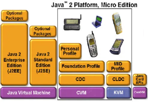
(10) Chapter 1 Introduction In this chapter, some introduction materials are presented to help readers understand the essential concepts behind and the terms in the title of our research. First, we give an overview of the current status of the Java technology in embedded environment. Second, we explain the meaning of mixed-mode, which actually combines interpretation and just-intime (JIT) compilation, and the reason it suits for embedded JVM. Third, we discuss dual instruction set, an issue that is specifically relevant to embedded processors. After the introduction comes our research motivation and objectives. Finally, organization of this thesis is provided.. 1.1 Embedded Java Environment Developed by Sun in 1991, Java technology has evolved rapidly and becomes popular in all application fields, such as desktop PCs, powerful large-scale server, or even in small portable consumer devices. Recognizing the fact that different application fields possess different characteristics and demands, Sun in 1999 has grouped Java technologies into the Java 2 platform [1], which consists of three editions as in Figure 1-1, and each of which aims at a specific area: • Java 2 Enterprise Edition (J2EE) - targeted at scalable, transactional, and databasecentered enterprise applications with an emphasis on server-side development. • Java 2 Standard Edition (J2SE) - targeted at conventional desktop applications. • Java 2 Micro Edition (J2ME) - targeted at embedded and consumer devices, such as wireless handhelds, PDAs, TV set-top boxes, and other devices that lack the resources to support full J2SE implementation.. 1.

(11) Figure 1-1. Java 2 Platform (extracted from Sun). To address the diversity of large embedded world, which covers a wide range of devices, J2ME specifies two configurations: Connected Limited Device Configuration (CLDC) and Connected Device Configuration (CDC). Each configuration targets at different types of devices and therefore provides different class libraries and APIs. Table 1-1 gives an overview of the differences of the two configurations.. Table 1-1. J2ME Configurations Configurations Name. Connected Device Configuration (CDC). Connected Limited Device Configuration (CLDC). Target Devices. high-end PDAs, set-top cell phones, two-way pagers, boxes, screen phones, and etc. low-end PDAs, and etc.. Typical Memory Requirement. 2MB~16MB. 128KB ~ 512KB. Target Processor Type. 32-bit. 16-bit, 32-bit. Reference Virtual Machine. CVM. KVM. Other Features. high bandwidth network connection, most often based on TCP/IP. limited, low bandwidth network connection. 2.

(12) 1.2 Embedded Mixed-Mode Execution JVM Although the JVM can be easily realized by an interpreter, its slow performance is always a concern in performance-aware system. In order to overcome this problem, some compilation technologies must be applied. Ahead-of-time (AOT) compilers [2] allows offline compilation, so no run-time compilation overhead is needed. Conventional JIT compilers translate bytecode into machine code on the fly, and incorporate more optimization techniques for better performance with the expense of VM code size increase and run-time compilation overhead. However, memory-constrained JVM can tolerate neither the static compiled code size expansion imposed by AOT compilers nor the code size/compilation overhead imposed by conventional JIT compilers. The approach of mixed-mode execution in [3][4] relies an interpreter to execute interpreted code for some parts of the program, and also executes compiled code dynamically produced by a JIT compiler for the remaining parts. The line between a conventional JIT compiler and a JIT compiler that supports mixed-mode execution is, in actuality, indistinct. Nevertheless, the principles of mixed-mode execution can be clarified as follows. • Performance-critical parts of the program are compiled by a JIT compiler, and then natively executed. • Non-performance-critical parts of the program are interpreted by a interpreter. • Close interactions between the JIT compiler and the interpreter is necessary. As discussed in Section 1.1, embedded JVM (including its class libraries) has very limited memory budget, usually in the range of hundreds of kilobytes. For this reason, embedded JVM usually employs merely an interpreter as its execution engine. But with the increasing demands for speed performance, embedded JVM also seeks ways to improve its slow execution speed. The most effective way is to incorporate a JIT compiler, as most desktop/server JVMs do. Still, taken limited memory resources into consideration, a fullfledged JIT compiler does not suit for an embedded JVM. Therefore, a lightweight JIT compiler, which is highly-customized for an embedded JVM, is needed. To this end, a mixed-mode JVM seems to be promising in embedded environment. By tightly coupling 3.

(13) with an interpreter, a JIT compiler can reuse the interpreter-based JVM as its infrastructure, in order to keep itself compact. And overall the combination (an interpreter-based JVM and a JIT compiler) builds up an embedded mixed-mode JVM.. 1.3 Dual Instruction Set For Code Size Reduction Due to the requirements of low manufacturing cost, low power consumption, and small volume size, embedded systems usually have limited hardware resources, especially in memory size. 8-bit, 16-bit MCU processors have dominated the embedded system for a long time. However, with the increasing demands on more data applications in high-performance embedded system, 32-bit embedded processors have become mainstream these days. Most 32-bit embedded processors are RISC-based, which suffer from the problem of poor code density and thus require more memory space. This is a severe limitation for costsensitive embedded systems. An innovative solution in architectural level is to employ “dual instruction set” [5]. One, the full instruction set, contains original 32-bit instruction set; the other, the compressed instruction set or the reduced bit-width instruction set, encodes most commonly used instructions in fewer bits (usually 16 bits). According to previous researches, a program compiled in compressed instruction set will be much smaller than that in full instruction set. For example, the code size reduction of Thumb/ARM is 30% [6], while the case of MIPS16/MIPS32 is 30%~40% [7]. However, due to a limited set of instructions and access to a limited set of registers, a program will be compiled into more instructions in the compressed instruction set, which may result in overall performance degradation. Therefore, how to effectively facilitate dual instruction set to keep a balance between code size and performance, is both a practical industrial problem and a hot research topic.. 4.

(14) 1.4 Research Motivation and Objectives Our observations are that while an embedded JVM manages to improve its execution speed, it still faces the problem of limited memory resources. Motivated by this fact, our objective is to design and implement an embedded JVM, which is small footprint compared to other existing embedded JVMs. We employ mixed-mode execution in our embedded JVM and further facilitate the “dual instruction set” feature that hardware architectural provides, aiming at striking a balance between speed performance and memory usage. In addition, some practical decisions of our research are listed as follows. • Our focus is on the design and implementation of a baseline JIT compiler for an embedded mixed-mode JVM, based on Sun’s CLDC KVM 1.0.4 (interpreter-based). For ease of reference, the JIT compiler is hereafter termed KJITC, an abbreviation for “Kilobyte Just-In time Compiler”. • KJITC targets the ARM/Thumb dual instruction set processor.. 1.5 Organization of This Thesis The remaining parts of this thesis is organized as follows. Chapter 2 provides more detailed background knowledge on JVM internals and common JIT compiler optimizations. In Chapter 3, the design of KJITC is presented along with speed performance analysis and the design of ARM/Thumb instruction setction. In Chapter 4, experiemnt results are exhibited. In the end we make a brief summary in Chapter 5.. 5.

(15) Chapter 2 Background This chapter provides more background details on JVM internals and JIT compiler optimizations. Readers who are already farmiliar with the two topics can skim over them. Also some related researches on dual instruction set and embedded JVM are discussed in the last section.. 2.1 Java Technology Although generally used to refer to a computer language, Java is a rather a complete architecture in reality. It consists of four distinct but interrelated components [8]. • Java programming language • Java class file format • Java Application Programming Interface (Java API) • Java Virtual Machine (JVM) A Java program is written in Java programming language, and then compiled into Java class files by Java source compiler. Java class files can be executed on any environment that equips a JVM. Also, the Java program can access predefined libraries or system resources (such as I/O, for example) by calling methods in the classes that implement the Java API. During program execution, JVM loads and executes user-written class files as well as these system classes that Java API defines.. 2.1.1 JVM Benefits Java Virtual Machine is definitely the key component among the all. It is responsible for the well-known advantages that Java possesses over traditional native execution system. Those advantages include: 6.

(16) • Cross-Platform Portabilty Each type of processor has its unique instruction set. For example, the instruction set of x86 is not compatible with that of MIPS. Moreover, each operating system (OS) has its own application interface or system calls to upper application programs. As a result, programs compiled to run on one platform (combination of processor and OS) cannot be executed on others without recompilation. Java overcomes this limitation by inserting JVM between the application programs and the real environment. If JVM has been ported to the environment, Java programs can be first compiled to Java bytecode in the form of class files and then be executed over the JVM without any porting efforts. This encourages software reuse and alleviates great pains from programmers.. • Security of the Execution Environment One of Java’s original intention is its integration into the network environment. In this environment, class files can be automatically downloaded from network and be locally executed. They might be malicious and might do dangerous operations to the local execution system. To deal with this important issue, Java build up its own security model - the sandbox [9][10]. As a brief explanation, Java verifies every class file from untrusted resources. The verification process mainly involves two steps in JVM. First, class file verification checks the layout and the contents of the class file. Second, bytecode verification checks if the bytecode within a method adheres to predefined rules. For example, one basic rule is that all goto and branch instructions refer to valid bytecode addresses.. • Small Size of the Compiled Code Due to the rich semantics and the stack-based operations, Java bytecode, the instruction set of JVM, is more compact space-wise than a statically compiled program. In other words, Java has high code density. According to [11], the dynamic average instruction size is 1.8 bytes. Compared with typical RISC instruction requiring 4 bytes, this result is satisfactory. For a speed-limited network environment or a memory constrained embedded. 7.

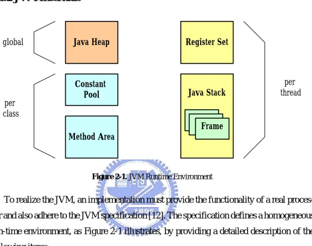
(17) environment, small code size is undoubtedly favorable.. 2.1.2 JVM Internals. global. per class. Java Heap. Register Set. Constant Pool. Java Stack. per thread. Frame Method Area. Figure 2-1. JVM Runtime Environment. To realize the JVM, an implementation must provide the functionality of a real processor and also adhere to the JVM specification [12]. The specification defines a homogeneous run-time environment, as Figure 2-1 illustrates, by providing a detailed description of the following items: • Instruction Set (Java Bytecode) • Register Set • Java Stack • Execution Environment • Constant Pool • Method Area • Java Heap • Object Management and Garbage Collection. 8.

(18) Since the JVM is a stack-based architecture, the registers of its register set are not used for storing operands or passing arguments as in most register-based machine. They only hold the state of the JVM and are updated after every bytecode instruction is executed. The operands of a bytecode instruction must be pushed onto the Java stack before the instruction is executed. An executing instruction consumes its operands from the stack and then places results on the stack when it completes. The execution environment is maintained within the Java stack as a data set and is used to deal with dynamic linkage, method invocation/return and exception handling. It handles dynamic linkage by maintaining symbolic references to methods and variables for the current method and current class. A symbol table is used to translate these references to actual calls. The JVM maintains a special table for each class, known as a constant pool. The constant pool contains string literals, class names, field names and other constant data objects that are referred to by the class structure or by the executing program. These constants do not change, and are created at compile-time. Items in the constant pool encode all names used by any method in a particular class. The information included in a class is the number of constants and the offset that specifies where a particular list of constants begin in the class description. The method area is equivalent to the compiled code areas in the run-time environment used by other programming language. It contains bytecode instructions that are associated with the methods in the compiled code and the symbol table needed for dynamic linkage. The Java heap is the dynamic memory of JVM, and it usually contains a collection of objects. When an object is created with the “new” bytecode instruction, an reference to that object is returned. This reference can be used subsequently, or stored in the current frame. An object persists in Java heap until there are no references to it in any frame of the frame stack or in the constant pool of any visible object. When there are no such references, an object becomes garbage, and a special garbage collector will reclaim its resources.. 9.

(19) 2.1.3 JVM Implementation Alternatives The JVM is not restricted to software interpreter implementation. In fact, there are three common approaches, as depicted in Figure 2-2, to implement the JVM.. Java Program Java Compiler. Machine Binary. Operating System. General CPU. Operating System. ted xecu. iled omp. Interpreter. Java. E tly irec 3. D. Compiler. 2. C. 1. I nterp reted. Bytecode. Java CPU. An Executable Form Figure 2-2. Three Alternatives to Executing Java Programs (extracted and modified from [13]). Interpreting the bytecode, the standard way to implement the JVM, has the advantage of fast JVM porting but makes the execution of Java programs relatively slow. One solution to improve speed performance is to replace an interpreter with a bytecode compiler. The bytecode compiler is responsible for translating bytecode into native machine code. While ahead-of-time (AOT) compilers performs offline compilation statically as conventional compilers, just-in-time (JIT) compilers performs on-the-fly compilation dynamically. Both of them have pros and cons, but JIT compilers seem to be more appealing to most researchers. Another solution is to implement the JVM directly on silicon. For example, picoJava is a Java processor that supports bytecode execution completely. As discussed in Section 1.2, an interpreter can still coexist and cooperate with a JIT compiler in the JVM. Recently, a mixed software/hardware approach also comes to exist. ARM has introduced its own Java instruction extension - Jazelle [14]. A subset of bytecode 10.

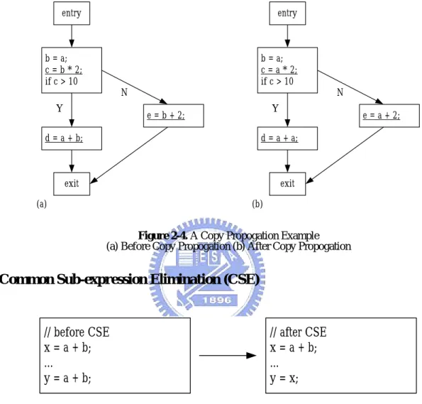
(20) instructions can be directly executed when the ARM processor is operated in Java mode, and the remaining bytecode instructions are still handled in software (interpreted or compiled).. 2.2 JIT Compiler Optimizations Since JIT compilers perform compilation at run time, the restriction of compilation time is more severe than that in traditional static compilers. As a result, only cost-effective optimization techniques can be suitably applied during JIT compilation. Due to the characteristics of Java, optimization techniques might cause different impact when applied in Java JIT compilers than in traditional static C compilers. In this section, we are to discuss some common optimization techniques used in Java JIT compilers [15][16][17], and then to discuss different ranges of optimization.. 2.2.1 Common Optimization Techniques Constant Folding The concept behind constant folding is to evaluate constant expression, whose operands are known to be constant, at compile time. After this simple transformation, the constant expression is replaced by its value. Therefore it saves the run-time computation of the expression. A simple example is demonstrated in Figure 2-3.. // before constant folding x = 10 + 2;. // after constant folding x = 12;. Figure 2-3. A Constant Folding Example. Copy Propagation Copy propagation is a transformation that replace variable occurrences with its copy value which is defined in earlier copy assignments. For example, the copy assignment is represented in the form x = y, for some variables x and y. Then later uses of x, as long as intervening instructions have not changed the value of either x or y, can be replaced with y. 11.

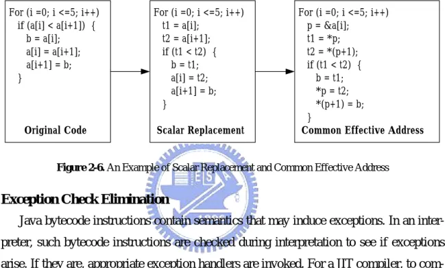
(21) Figure 2-4 is an example in the flowgraph form. The copy assignment is b = a, and succeeding occurrences of b of the underlined expressions are replaced with a.. entry. entry. b = a; c = b * 2; if c > 10. b = a; c = a * 2; if c > 10 N. Y. N Y. e = b + 2;. d = a + b;. e = a + 2;. d = a + a;. exit. exit. (a). (b). Figure 2-4. A Copy Propogation Example (a) Before Copy Propogation (b) After Copy Propogation. Common Sub-expression Elimination (CSE). // before CSE x = a + b; ... y = a + b;. // after CSE x = a + b; ... y = x;. Figure 2-5. An Example of CSE. The purpose of CSE is to reduce repetitive computations by substituting available results for the expressions that do the same computation. Figure 2-5 gives a simple example. Also two common derivatives of CSE are: • Scalar Replacement Array element accesses in a loop are replaced by temporary variables, when the array objects and the array indexes remain unchanged. See the example in Figure 2-6.. 12.

(22) • Common Effective Address Generation Successive array element accesses in a loop can be optimized by introducing a temporary pointing to the first element. Therefore other elements can be accessed by using the temporary as the base address and corresponding array indexes as offsets. See the example in Figure 2-6.. For (i =0; i <=5; i++) if (a[i] < a[i+1]) { b = a[i]; a[i] = a[i+1]; a[i+1] = b; }. For (i =0; i <=5; i++) t1 = a[i]; t2 = a[i+1]; if (t1 < t2) { b = t1; a[i] = t2; a[i+1] = b; }. Original Code. Scalar Replacement. For (i =0; i <=5; i++) p = &a[i]; t1 = *p; t2 = *(p+1); if (t1 < t2) { b = t1; *p = t2; *(p+1) = b; } Common Effective Address. Figure 2-6. An Example of Scalar Replacement and Common Effective Address. Exception Check Elimination Java bytecode instructions contain semantics that may induce exceptions. In an interpreter, such bytecode instructions are checked during interpretation to see if exceptions arise. If they are, appropriate exception handlers are invoked. For a JIT compiler, to compile these bytecode instructions also produce compiled code that performs exception check. However, some of these checks are redundant and can be eliminated via careful analysis. In short, exception check elimination helps to save unnecessary operations and also reduce code size. Null pointer check elimination and array bound check elimination are the most common techniques used in Java JIT compilers.. Method Inlining The idea of method inlining is to inline method calls by expanding method bodies. This optimization can reduce method invocation overhead in sacrifice of code size expansion and also can provide more optimization opportunities. In object-oriented languages like Java, tiny methods such as class constructors and methods that accesses private variables are frequently executed. These methods spend more time on method invocation than 13.

(23) method body execution. Hence method inlining is useful under these circumstances. Moreover, concerning the heavy overhead of devirtualization, virtual method calls may be inlined as well. Certainly, it involves further analysis.. Strength Reduction and Machine Idioms Strength reduction is to replace an operation with a semantically equivalent one, though weaker but faster. A common case is using the shift operator to multiply and divide integers by a power of 2. For example, x >> 2 can be used in place of x / 4, and x << 1 replaces x * 2. In a similar way, machine idioms refer to instructions or instruction sequences for a specific ISA that executes more efficiently than a similar sequence of instructions targeted for a more general architecture. A good example is that some architectures provide multiply-and-add instructions for faster execution.. 2.2.2 Optimization Range Conventionally, an optimization applied to a program is generally called "local" if it is performed by looking only at the statements in a basic block; otherwise, it is called "global" [18]. To be more specific, "local" means optimization is applied within a basic block while "global" within a function. Some optimization techniques can be applied at both local and global levels. Global optimization invests more compilation time in advanced analysis, and therefore leads to better compiled code quality. Local optimization might expand its optimization range from a basic block to an extended basic block [19]. As a contrast to single-entry-single-exit basic blocks, extended basic blocks are also single-entry but possibly multiple-exit, and therefore have more opportunities for optimization. Researches on high performance architectures focus on loop optimization in a program. In fact, high-level loop structures may be recovered by identifying strongly connected components (SCCs) or regions in a low-level control flow graph. Furthermore, interprocedural optimization is more aggresive for its range expands across functions, and thus is considered to be pretty costly. In short, as the optimization range is enlarged from local to loop and global, or even interprocedural, the cost of analysis definitely increases. For more detailed information, please also refer to [19].. 14.

(24) 2.3 Related Researches This section briefly introduces the essentials about dual instruction set and its current research status. Next, advancements in optimization for embedded JVM is discussed as well, including one recent research work on embedded JIT compilation.. 2.3.1 Dual Instruction Set A number of 32-bit RISC processors for embedded systems may incorporate a reduced bit-width instruction set as an architectural extension, and therefore support dual instruction set. ARM provides its 16-bit instruction set extension called Thumb since its ARM7 processors in 1995. With a decompression engine, Thumb instructions are converted to its ARM equivalents during decode pipeline stage. Switching between the two instruction sets is achieved through the use of explicit mode change (ARM mode and Thumb mode) insructions. Thumb instructions are only able to access 8 general purpose registers (out of 16) without any restrictions, and can only encode small immediate values. Also addressing modes and instruction types are restricted in Thumb instruction set. Experiment results exhibit with 32-bit memory Thumb trades off 30% - 40% speed performance for 30% code size reduction. MIPS follows ARM by offering its MIPS16 instruction set in 1997. As a contrast to Thumb, MIPS16 contains an extend opcode which extends the values of immediate operands that are not representable due to bit width constraints. Rather than switch with explicit mode change instructions, code alignment dictates the mode of execution. To be more specific, a function that is not word-aligned is assumed to be composed of MIPS16 instructions. Experiment results show the code size reduction is up to 40% using MIPS16. Other processors that support dual instruction set include the ST100 Core [20] from ST Microelectronics and the Tangent-A5 [21] from ARC. Two recent research papers [22][23] about dual instruction set are on evaluation of mixed instruction set code in different granularities such as function levels and basic block levels. Their proposed heuristics for instruction set selection are static, profile guided and may be based on cost models. However, no apparent results can be inferred from the 15.

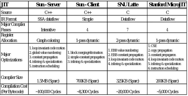
(25) researches about how to perform instruction set selection for specialized environments such as a mixed-mode JVM. This also serves as a reason that motivates us to conduct this research work.. 2.3.2 Embedded JVM Due to tight memory constraints, embedded JVM usually seeks its way for performance improvement by adopting low-cost optimizations in terms of code size. These low-cost optimizations manage to improve overall performance by reducing overheads in exception handling, garbage collection, object access and bytecode dispatch. Among of them, optimization for bytecode dispatch is most effective since dispatch time occupies a great portion of total execution time. Researches in [24][25] discuss different threading mechanisms to improve dispatch efficiency for JVM. Moreover a bytecode instruction sequence can be grouped together or formed into a new bytecode, and therefore only one dispatch is necessary as described in [26]. Since the sequence is executed as a whole, there are opportunities that it can be executed more efficiently by optimizing native code. Related works of this type include [27][28]. Although aforementioned optimizations can be employed in embedded JVM without much code size expansion, their performance improvement is potentially and relatively low compared with JIT compilation. As a result, for embedded JVM that demands high performance, JIT compilation is indispensable. A recent work [29] demonstrates a JIT compiler designed for employment in embedded JVM. Table 2-1, which is extracted and modified from the same work, lists some important features of this embedded JIT compiler compared with other JIT compilers. Apparently the embedded JIT compiler consumes much code size such that highly-memory-limited embedded systems can not afford. Therefore, there is still research space for more lightweight JIT compilation that can be applicable to a wider range of embedded systems with JVM.. 16.

(26) Table 2-1. Comparison Among Some JIT Compilers JIT Source IR Format Major Compiler Passes Register Allocation Major Optimizations. Compiler Size Compilation Cost (Per Bytecode). Sun - Server. Sun - Client. SNU Latte. Stanford MicroJIT. C++. C++. C. C. SSA dataflow. Simple. Dataflow. Dataflow. Interative. 4. 7. 4. Graph coloring. 1-pass dynamic. 2-pass dynamic. 1. loop invariant code motion 1. block merging/elimination 2. global value numbering 2. simple constant propagation 3. constant propagation 3. inlining & specialization 4. inlining & specialization 5. instruction scheduling. 1. EBB value numbering 2. EBB constant propagation 3. loop invariant code motion 4. inlining & specialization. 1-pass dynamic 1. CSE 2. copy propagation 3. constant propagaron 4. loop invariant code motion 5. inlining & specialization 6. instruction scheduling. 1.5MB (Sparc). 700KB (Sparc). 325KB (Sparc). 200KB (Sparc). ~100,000 Cycles. ~8,300 Cycles. ~20,000 Cycles. ~5,000 Cycles. 17.

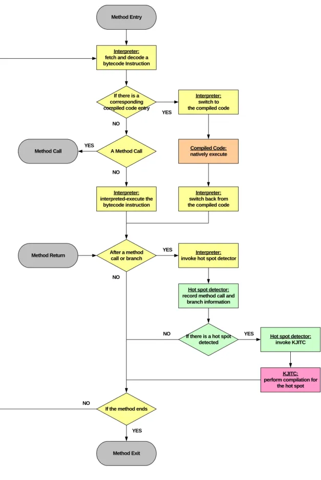
(27) Chapter 3 System Design In this chapter, we present the overall system design of our embedded mixed-mode JVM. Section 3.1 provides an overview of our system, which consists of four components, and then discusses their relative interactions. Section 3.2, a quantitative analysis on speed performance of our system, compared with that of a pure interpreter-based JVM, is proposed. The analysis helps us make our further design decisions in KJITC. Next, we detail the internal design of KJITC and its optimizations. Finally, we demonstrate design issues on ARM/Thumb instruction set selection.. 3.1 System Overview Time Interpreter: interpret Java bytecode. invoke hot spot detector Hot Spot Detector: detect a hotspot. resume interpretation. invoke KJITC KJITC: perform hotspot compilation. Interpreter: interpret Java bytecode switch between interpreter and compiled code. Compiled Code. Interpreter: interpret Java bytecode. Figure 3-1. System Components and Their Interactions. In our mixed-mode embedded JVM, there are four main components. Their interactions can be simply illustrated in Figure 3-1. A more precise flowchart which describes the working flow during method interpretation is also provided in Figure 3-2 for completeness. 18.

(28) Method Entry. Interpreter: fetch and decode a bytecode Instruction. If there is a corresponding compiled code entry. YES. Interpreter: switch to the compiled code. NO. YES Method Call. Compiled Code: natively execute. A Method Call. NO. Interpreter: interpreted-execute the bytecode instruction. Interpreter: switch back from the compiled code. YES. After a method call or branch. Method Return. Interpreter: invoke hot spot detector. NO Hot spot detector: record method call and branch information. NO. If there is a hot spot detected. YES. Hot spot detector: invoke KJITC. KJITC: perform compilation for the hot spot NO If the method ends. YES. Method Exit. Figure 3-2. System Flowchart. 19.

(29) Now we respectively discuss each component as follows. • Interpreter-based JVM (KVM) The interpreter-based JVM provides a JVM infrastructure that performs exception handling, garbage collection, synchronization and etc. It comes with a simple interpreter as its execution engine. For mixed-mode execution, the interpreter must be responsible for invoking the hot spot detector and switching to/form compiled code in addition to interpretation of those bytecode that have not been compiled or will not be compiled. • Hot Spot Detector Due to the tight memory constraints, only valuable parts of the input program are selected for JIT compilation. By the 80/20 rule, over eighty percent of execution time is spent in less than twenty percent of source code in a program. Apparently, the responsibility of the hot spot detector is to discover these performance-critical twenty percent of source code and then invoke JIT compiler for hot spot compilation. As mentioned in Section 2.1.2, the method area is viewed as the run-time compiled code area. Hence we also select the method as the basic unit of hot spot detection. A method is considered to be a hot spot, when it meets either one of the following two requirements. First, it is called by other methods frequently. Second, it contains at least one loop that has many iterations. In our implementation, threshold values must be set statically as the criteria for the two requirements. Currently the values are both chosen to be 40, which are based on our evaluation results. • JIT Compiler (KJITC) The JIT compiler is further divided into the IR (Intermediate Representation) generator and the native code generator. The IR generator is mainly responsible for translating Java bytecode into semantically equivalent three-address IR. And then the code generator translates IR into targeted native code for later execution. A simple illustration is given in Figure 3-3.. 20.

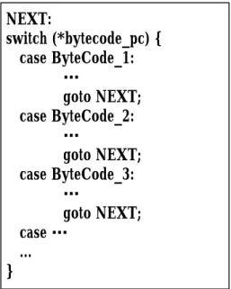
(30) Three-address IR Java Bytecode Targeted Native Code (ex. ARM). IR Generator. Native Code Generator. Figure 3-3. An Illustration of KJITC. • Compiled Code Buffer The compiled code buffer holds all compiled native code. During native execution, the machine program counter (PC) points to native code that resides in the buffer. In our current implementation, the compiled code buffer is allocated statically, and its size is also predetermined. In addition to the four components, the switching mechanism between the interpreter and the compiled native code also deserves discussions. Similar to a function call, the switch from the interpreter to the compiled native code involves spilling registers into memory and then transfering execution by a branch. The case of the switch from the compiled native code to the interpreter involves more operations. It has to restore registers from memory, to transfer execution by a branch, and to update Java PC (program counter) and Java SP (stack pointer).. 3.2 Speed Performance Analysis Before proceeding to the focus of our research - the KJITC, we present basic quantitaive analysis of system performance in this section. First we begin with an interpreter-based system, and then compare it with our system, which exhibits mixed-mode execution.. 21.

(31) 3.2.1 Interpreter-Based JVM NEXT: switch (*bytecode_pc) { case ByteCode_1: … goto NEXT; case ByteCode_2: … goto NEXT; case ByteCode_3: … goto NEXT; case … ... } Figure 3-4. The Interpreter Dispatch Loop. Figure 3-4 shows a simplified dispatch loop - the main structure of an interpreter - in C language source form. An interprter may be viewed as a software processor that sequentally performs three tasks - fetching, decoding, and execution. For ease of reference and explanation, we delibrately break the total execution time of an interpreter-based JVM into the following three parts. Figure 3-5 is a timing diagram of an interpreter-based JVM which performs bytecode interpretation in a repetitive manner. • Dispatch (fetching + decoding) time ... Tdisp => Dispatch time of a single bytecode instruction ... tdisp • Interpreter execution time ... Tint_exec => Average interpreter execution time of a single bytecode instruction ... tint_exec • Miscellaneous time ... Tmisc (garbage collection, synchronization, and etc.). 22.

(32) Interpreter. .... T disp. T int_exec. T disp. T int_exec. ... time. Figure 3-5. Timing Diagram of the Interpreter-based JVM. 3.2.2 Mixed-Mode Execution JVM Similarly, the breakdown of the total execution time in our mixed-mode execution JVM can be listed as the following six parts. Figure 3-6 is a typical timing diagram which comprises the leading five parts while omitting miscellaneous time for clarity. • Dispatch (fetching + decoding) time ... T'disp • Interpreter execution time ... T'int_exec • JIT compilation time ... Tcomp • Interpreter-native code switch time ... Tswitch (Tswitch_from + Tswitch_to) => One switch time ... tswitch (tswitch_from + tswitch_to) • Native code execution time ... Tnative_exec => Average native code execution time of a single bytecode instruction ... tnative_exec • Miscellaneous time ... T'misc. Compiled Code JIT Compiler Interpreter. T native_exec. T comp. .... T' disp. T switch_from. T switch_to. .... T' disp. T'int_exec. Figure 3-6. Timing Diagram of the Mixed-mode Execution JVM. 23. ... time.

(33) 3.2.3 Speedup of Mixed-mode Execution Over Interpreter-Execution To compare relative performance of the mixed-mode execution JVM and the interpreter-based JVM, following speedup definition is provided.. Speedup of A over B =. Execution Time of B Execution Time of A. Then the speedup of the mixed-mode execution JVM over the interpreter-based JVM can be expressed as follows.. Speedup. (overall). =. Tdisp + Tint_exec + Tmisc T' comp + T' disp + Tint_exec + Tswitch + Tnative_execc + T' misc. For a compiled sequence of n bytecode instructions, speedup can be approximated by the following equation.. Speedup. (block). =. Tdisp + T int_exec n × tdisp + n × tinit_exec = T' disp + Tswitch + Tnative_exe cc tdisp + tswitch + n × tnative_exe c. For further analysis, some values in the above equation can be obtained in our implementation. Then the equation becomes:. Speedup. (block). =. ( 21n ) + T int_exec ( 21) + (53 ) + T native_exe c. The meaning of the equation is that: • It takes 21 cycles for every bytecode interpretation and some varied cycles for interpreted execution. • It takes 21 cycles for identifying a sequence of compiled code, and the overall switching time is 53 cycles, plus some varied cycles for native execution. With the equation, we make some discussions as follows.. 24.

(34) • Since most bytecode instructions only involve simple operations, such as IADD, ILOAD, and ISTORE, the average interpreter execution time of a bytecode instruction is fewer than 21 cycles. As a reference, it is statically and roughly estimated to be 9.7 cycles in our implementation. According to Amdahl's law, the performance bottleneck is the dispatch time, Tdisp. Therefore, the first priority is to reduce the dispatch overhead by enlarging the value of n. • The time of interpreted execution is definitely larger than that of native execution, for the JIT compiler can perform optimizations while the interpreter cannot. The value of Tint_exec over Tnative_exec may be roughly referred as the code quality of the compiled code. In theory, when n = 1, the code quality shall be equal to 1, since there is no room for optimization. Conversely, when n grows larger, the code quality may grow larger as well. Therefore, the second priority is to improve the code quality, either by enlarging the value of n or by employing more optimizations. As a motivating example, we consider the bytecode sequence of "ILOAD_1, ILOAD_2, IADD, ISTORE_1". The values of Tint_exec and Tnative_exec can be simply computed in our implementation, assuming that instruction folding for stack operation in Section 3.4.1 is applied during compilation. Now the equation can be evaluated.. Speedup. (block). =. ( 21 × 4) + (33) = 1.24 ( 21) + (53) + (9). From the above equation, we can compute the average values - tint_exec and tnative_exec, and then re-build up the speedup equation.. Speedup. (block). =. ( 21n ) + ( 6 n ) ( 27 n ) = ( 21) + (53 ) + ( 2 .25 n ) ( 74 ) + ( 2 .25 n ). When the value of n equals to 20, the speedup is about 4.54. When the value of n equals to 50, the speedup is about 7.24. Figure 3-7 is a plot that exhibits the trend of speedup when n increases.. 25.

(35) 102 4. 512. 256. 128. 64. 32. 16. 8. 4. 2. 1. Speedup. 14 12 10 8 6 4 2 0. the value of n. Figure 3-7. The Trend of Speedup. As the plot shown, the speedup will coverge as the value of n increases. Although this ideal speedup trend may differ from that in real cases, it still provides some useful guidelines when designing our baseline KJITC.. 3.3 KJITC Architecture IR Generator (1st Pass) Function:. Native Code Generator (2nd Pass) Function:. Java translation of Java bytecode Bytecode into semantically equivalent. 3-address 1. register allocation/assigment 2. instruction selection/ IR. 3-address IR. Targeted Native Code (eg. ARM). generation. Optimizations: 1. rule-based null pointer check elimination 2. strength reduction. Optimizations: 1. instruction folding for stack operations 2. constant propagation 3. constant folding. Figure 3-8. Two-pass Compiler Architecture. In this section, we detail the design of the IR generator and the native code generator in the KJITC. In addition, in order to reduce compilation cost and to keep the KJITC small26.

(36) footprint, several design decisions are made based on the analysis in Section 3.2. These decisions are: • Two-pass Compiler Architecture We confine our compiler to two passes. The first pass is for IR generation, and the second pass is for native code generation. Figure 3-8 gives a more detailed overview of functions and optimizations of the two passes. This decision is based on the fact that fewer passes take less compilation time and that two passes seem to be reasonable for portability. The IR generator is responsible for translating Java bytecode into machine-independent three-address IR, and therefore is portable across platforms. Clearly the KJITC needs only one IR generator while possessing more than one native code generator for different targeted architectures as depicted in Figure 3-9.. IR Generator. ARM Code Generator. Thumb Code Generator. MIPS Code Generator. Figure 3-9. One IR Generator With Many Native Code Generators. • Only Local Optimization Within an Extended Basic Block No global optimization is performed due to the potential high compilation cost of control and data flow analysis. However, we extend the maximum optimization range to an extended basic block rather than a basic block. • Support for More Bytecode If the KJITC can compile more types of bytecode, compilation may be possibly applied to a longer sequence of input bytecode, which in turn results in better performance as we have discussed in Section 3.2.3. • No Support for Complex Bytecode 27.

(37) Complex bytecode refers to those bytecode instructions that involve complicated operations that suit for interpreter handling. These complicated operations include devirtualization, synchronization, object construction/destruction, and etc. As a result, these complex bytecode instructions are considered to be non-compile-able in the KJITC.. 3.3.1 IR Generator IR Format The IR format is designed with the following two properties. • Three Address Quadruple: (Opcode, Arg1, Arg2, Arg3) Opcode refers to the instruction operation. Arg1 generally refers to the destination of the operation. Arg2 generally refers to the first source of the operation. Arg3 generally refers to the second source of the operation. • Local-Variable-Based Memory Addressing Arg1, Arg2, and Arg3 are used for storing constants or memory addresses. The memory addresses are local-variable-based. That is, the actual values stored are the offsets relative to the base address of the local variable array. In the KVM, the operand stack and the local variable array of a frame both reside in a linearly addressable range of memory, and thier relative addresses are also fixed (see Figure 3-10). During the execution of a program, frames are dynamically created and discarded, hence their memory addresses can only be determined at run-time. As a result, elements of the local variable array and the operand stack are addressed by using the starting address of local variable array as the implicit base address plus corresponding word-offsets encoded in instructions.. 28.

(38) stack growth top of stack ... .... operand stack. Entry #(n+1) Entry #n base of stack. frame frame struct attributes ... .... base of local variable array. local variable array. Entry #0. Figure 3-10. The Frame Structure in Memory. Bytecode to IR Translation After the design of IR format is decided, bytecode can be easily translated into semantically-equivalent IR. Much of the work involves translation from implicit stack addresses into explicit local-variable-based addresses. Following are some examples for demonstration. 1. DUP • Bytecode Number: 89 • Function: To duplicate the top element of the operand stack • Translated IR: (MOV, &TOS[0]-&LV[0], ---, &TOS[-1]-&LV[0]) • Brief Description: The IR operation is MOV. The destination of the operation is the empty element of the operand stack. Since the top-of-stack pointer always points to the empty element of the operand stack, the destination can be addressed by &TOS[0]&LV[0]. The first source of the operation is unused, and the second is the top element of the operand stack which is addressed by &TOS[-1]-&LV[0]. 2. ILOAD_1 29.

(39) • Bytecode Number: 27 • Function To push the second local variable onto the operand stack • Translated IR: (MOV, &TOS[0]-&LV[0], ---, &LV[1]-&LV[0]) • Brief Description: The IR operation is MOV. The destination of the operation is the empty element which is addressed by &TOS[0]-&LV[0]. The first source of the operation is unused. The second source of the operation is the second local variable which is addressed by &LV[1]-&LV[0]. 3. IADD • Bytecode Number: 96 • Function: to pop and add the top two elements from the operand stack, and then push the result back • Translated IR: (ADD, &TOS[-2]-&LV[0], &TOS[-2]-&LV[0], &TOS[-1]-&LV[0]) • Brief Description: The IR operation is ADD. The destination and first source of the operation is the second top element of the operand stack which is addressed by &TOS[2]-&LV[0]. The second source of the operation is the first top element of the operand stack which is addressed by &TOS[-1]-&LV[0]. It is worth noting that a semantically-rich bytecode instruction may be decomposed into several simple IR instructions. For example, bytecode instructions for array access involve implicit exception checks, and therefore their decomposed IR instructions contain explicit exception checks.. 30.

(40) IR Generation Workflow A Hot Spot Method. A non-compilable bytecode. A compilable bytecode. An IR Block. An IR Block. An IR Block. An IR block which consists of consecutive IRs. An IR Group (which consists of IR blocks). Figure 3-11. Input and Output of the IR Generator. As discussed in Section 3.1, the basic unit of hot spot detection is a method and then it is passed to the IR generator to generate corresponding IR. Figure 3-11 is an illustration that shows the input and the ouput of the IR generator. The detailed workflow is listed as the following steps. 1. The IR generator takes a hotspot method as input. 2. The IR generator linearly parses each bytecode instruction of the method and generates corresponding IR for compile-able bytecode. During the linear pass, the IR generator also updates the PC (program counter) and SP (stack pointer) information for each bytecode instruction. The information is then used by the switching mechanism described in the last paragraph of Section 3.1. For detailed PC and SP offset adjustments of each bytecode instruction, please refer to Appendix A. 3. Consecutively generated IR instructions are collected in a IR block. 4. After IR generation completes, all IR blocks are managed by a IR group. The IR group is then passed to native code generator for code generation. Since a progam has branch-type instructions, its control flow is not always sequential. In order to overcome this problem, it is necessary to to discover the control structure of the. 31.

(41) program by control-flow analysis. However, we reduce the extra cost of control-flow analysis by utilizing the StackMap attribute which is specified in the CLDC specification [30]. The StackMap attribute records (PC offset, SP offset) tuples for all branch targets in a method. Therefore the IR generator can use the information to identify extended basic blocks. This also implies the maximum range of an IR block is its corresponding extended basic block, provided that there are no intervening non-compile-able bytecode.. 3.3.2 Native Code Generator The main responsibility of the native code generator is to perform register allocation/ assignment and instruction selection/generation. Also some optimizations are applied in this stage. Since the native code generator is designed for one pass, it implies that register allocation/assignment is done within one pass and instruction selection/generation must be performed at the same time. To be more specific, the native code generator assigns registers as machine instructions are generated. The design of the register allocation/assignment scheme is simple, but highly customized for the JVM environemnt. Its detailed discussion is deferred until Section 3.4.1. After the IR generation phase, the native code generator receives an IR group as input for code generation. However, the basic unit for code generation is confined to an IR block. In fact, local optimizations in KJITC are all restricted to the range of an IR block. During the code generation for an IR block, the code generator parses each IR instruction and generates corresponding machine instructions, and it is also responsible for generating necessary register load/spill instructions. Besides, the native code generator also incoporates optimizations like constant folding and constant propagation which can help to generate better code. Upon the end of an IR block, the native code generator must spill registers for live variables. As an optimization technique, the native code generator only spills registers for variables whose memory addresses are below the current stack pointer, since variables above the current stack pointer will not be used again in the stack-based JVM.. 32.

(42) Similar to the IR generator, the native code generator collects consecutively generated native code for an IR block in a compiled code block. And all compiled code blocks are managed by a compiled code group. What is worthy of noting is that a compiled code block resided in the compiled code buffer is in reality the basic unit for native execution.. 3.4 KJITC Optimizations We devote this section to the design of major optimization techniques in KJITC. These two optimizations - stack operation folding and rule-based null-pointer check elimination are designed with the characteristics of the JVM in mind and thus are highly-customized and efficient.. 3.4.1 Instruction Folding For Stack Operations One characteristic of the stack-based JVM is all operations must be done within the Java stack. When mapping the stack-based architecture to the common register-based architecture, this imposes great restrictions and also leads to much inefficiency. Considering the bytecode sequence "ILOAD_0, ILOAD_1, IADD, ISTORE_0", its highlevel operations are illustrated in Figure 3-12 (a). If these operations can be simplified as shown in Figure 3-12 (b), the execution flow will become more efficient. This technique is called "stack operation folding" in researches on Java processors [31][32].. 33.

(43) stack growth. ALU. ALU 5. 3 4. producer 1. operand stack. 2 consumer. 2. 3 operand stack. 1 6. local variables. local variables. (a). (b). Figure 3-12. Stack Operations (a) Without Folding (b) With Folding. As a contrast, the bytecode sequence can be one-to-one translated into IR instructions as in Figure 3-13 (a). It is observed that the three copy assignments (IR_1, IR_2, and IR_4) can be folded into the third IR instruction by replacing corresponding source and destination fields. After the folding, only one IR instruction is needed instead of four, as in Figure 3-13 (b). This optimization is different from copy propagation in that copy propagation only allows IR_1 and IR_2 to be forward folded into IR_3 while it also allows IR_4 to be backward folded into IR_3.. Bytecode 1. 2. 3. 4.. ILOAD_0 ILOAD_1 IADD ISTORE_0. IR: (OP, 1. 2. 3. 4.. DST,. SRC1,. SRC2). (MOV, &TOS[0]-&LV[0], ---, &LV[0]-&LV[0]) (MOV, &TOS[1]-&LV[0], ---, &LV[1]-&LV[0]) (ADD, &TOS[0]-&LV[0], &TOS[0]-&LV[0], &TOS[1]-&LV[0]) (MOV, &LV[0]-&LV[0], ---, &TOS[0]-&LV[0]). (a). IR: (OP,. DST,. SRC1,. SRC2). 1. (ADD,. &LV[0]-&LV[0],. &LV[0]-&LV[0],. &LV[1]-&LV[0]). (b) Figure 3-13. IR Generation (a) Without Optimization (b) With Instruction Folding. 34.

(44) It is straightforward that the instruction folding technique can be employed in the KJITC by inserting one extra pass between the IR generation and the native code generation. However, devoting one extra pass for only one optimization technique is not cost-effective and also slows down compilation speed. Instead, we integrate this optimization in our native code generator. The register tracking scheme in our native code generator associates each register record with two two fields - one source and one destination. While encountering a MOVtype IR instruction, say the first IR instruction in Figure 3-13 (a), the code generator allocates/assigns a register, and records corresponding source and destination. Later, when the code generator sees the third IR instruction, it will use the allocated/assigned register as the first source. This way, unnecessary stack operations can be effectively removed. Compared with the register allocator in [33], ours is more lightweight and cost-effective. Figure 3-14 is a corresponding work flow of the aforementioned bytecode sequence.. Ｂｙｔｅｃｏｄｅ. １．ＩＬＯＡＤ＿０２．ＩＬＯＡＤ＿１３．ＩＡＤＤ４．ＩＳＴＯＲＥ＿０. IR translation. ＩＲ：（ＯＰ，ＤＳＴ，ＳＲＣ１，ＳＲＣ２）. １．（ＭＯＶ，＆ＴＯＳ［０］－＆ＬＶ［０］，－－－，＆ＬＶ［０］－＆ＬＶ［０］）ｒ１．ｄｓｔｒ１．ｓｒｃ２．（ＭＯＶ，＆ＴＯＳ［１］－＆ＬＶ［０］，－－－，＆ＬＶ［１］－＆ＬＶ［０］）ｒ２．ｄｓｔｒ２．ｓｒｃ３．（ＡＤＤ，＆ＴＯＳ［０］－＆ＬＶ［０］，＆ＴＯＳ［０］－＆ＬＶ［０］，＆ＴＯＳ［１］－＆ＬＶ［０］）ｒ１．ｓｒｃ＝ｒ１．ｄｓｔｒ１．ｄｓｔｒ２．ｄｓｔ４．（ＭＯＶ，＆ＬＶ［０］－＆ＬＶ［０］，－－－，＆ＴＯＳ［０］－＆ＬＶ［０］）ｒ１．ｄｓｔｒ１．ｓｒｃ Code Generation ＡｆｔｅｒｐａｓｓｉｎｇＩＲ＿１：ＡｆｔｅｒｐａｓｓｉｎｇＩＲ＿２：ＡｆｔｅｒｐａｓｓｉｎｇＩＲ＿３：. ＬＯＡＤｒ１，ＬＶ［０］ＬＯＡＤｒ２，ＬＶ［１］ＡＤＤｒ１，ｒ１，ｒ２. ＡｆｔｅｒｐａｓｓｉｎｇＩＲ＿４：ＳＴＯＲＥｒ１．ＬＶ［０］. Figure 3-14. Instruction Folding for Stack Operations During Code Generation. 35.

(45) 3.4.2 Rule-based Null Pointer Check Elimination Due to its architectural design, the JVM consists of many bytecode instructions that introduce. null. pointer. checks.. For. example,. in. KVM. "GETFIELD_FAST",. "PUTFIELD_FAST" are for object field access and "IALOAD", "IASTORE" for array element access, which overall impose much runtime overhead. To reduce such overhead, we propose a rule-based method which is employed in our IR generator. It can eliminate a great portion of IR instructions for null pointer checks in a cost-effective manner, in contrast to other methods employing data-flow analysis. Now the basic design of the method is described as follows. • Definition 1. Full Set: (F-Set) All compile-able bytecode instructions in the KJITC constitute this set. 2. Un-eliminated Set: (U-Set) All bytecode instructions in F-Set, which introduce null pointer checks by examining associated object references, constitute this set. 3. Target Set: (T-Set) A predetermined subset of U-Set. 4. Dominance Set: (D-Set) All bytecode instructions in F-Set, which produce object references that are later used by bytecode instructions in T-Set, constitute this set. 5. Influential Set: (I-Set) All bytecode instructions in F-Set, which may alter object references that are later used by bytecode instructions in T-Set, constitute this set.. • Data Structure. 36.

(46) 1.. A n-height stack (L-Stack) This is a tiny stack used to simulate stack operations. n poses a limit to the. maximum stack height that can be tracked. This stack is implemented as a n-element array. 2.. A m-bit-mask array (B-Array) This array, say array[0:m-1], is used to track whether the local variable 0 through. local variable m-1 is null pointer checked or not.. • Algorithm 1.. Select some bytecode instructions from U-Set as T-Set. 2.. Find the corresponding D-Set, I-Set. 3.. Upon an IR block entrance, initialize all n elements of L-Stack as "Not_Tracked".. When some bytecode instruction in D-Set is encountered, mark the corresponding element in L-Stack with the corresponding local variable number. 4.. Upon an IR block entrance, initialize all m bits of B-Array as "Un-Checked".. When some bytecode instruction in I-Set is encountered, mark the corresponding bit in B-Array with "Un-Checked". 5.. When some bytecode instruction in T-Set is encountered, if the bit mask of the. local variable associated with the object reference is "Checked", the null pointer check for this bytecode instruction is eliminated; otherwise the null pointer check remains and also the bit mask is then marked as "Checked". 6.. The flowchart of the algorithm is depicted in Figure 3-15.. 37.

(47) Begin. Fetch a Bytecode. End. NO. A Successful Fetch YES. Bytecode In F-Set. NO. YES. Initialize L-Stack and B-Array. YES. An IR block Entrance. NO. Bytecode In D-Set. YES. Mark Corresponding Entry in L-Stack with LV#. NO. Bytecode In I-Set. YES. Mark Corresponding Entry in B-Array with <Unchecked>. NO. NO. Bytecode In T-Set. YES. Replace the Corresponding Bit in L-Stack with <Checked>. NO. Corresponding Bit in L-Stack is <Checked>. YES. Eliminate Null Pointer Check. Figure 3-15. Flowchart of Null Pointer Check Elimination. 38.

(48) • A Simple Example 1.. Configuration: T-SET = {"GETFIELDP_FAST", "PUTFIELD_FAST" } D-SET = {"ALOAD", "ALOAD_0", "ALOAD_1", "DUP"} I-SET = {"ASTORE", "STORE", "ISTORE_0", "ISTORE_1"} Pick L-Stack as a 5-height stack Pick B-Array as a 4-bit-mask array. 2.. Given Code Sequence Within an IR-block (see Table 3-1): NT: Not Tracked NC: Not Checked (or Un-Checked) C: Checked. Table 3-1. An Example of Rule-based Null Pointer Check Elimination Byte-code. Stack Height (after execution). L-Stack (after execution). B-Array (after execution). Perform Null Pointer Check. <Initialize> ILOAD xxx ALOAD_1 GETFIELDP_FAST xxx IF_ICMPLT xxx ALOAD_1 ILOAD_2 PUTFIELD_FAST xxx ICONST_2 ISTORE_1 ALOAD_0 GETFIELDP_FAST 0x04 ICONST_0 ICONST_1 IASTORE. 0 1 2 2. {NT,NT,NT,NT, NT} {NT,NT,NT,NT, NT} {NT, 1, NT, NT, NT} {NT, 1, NT, NT, NT}. {NC, NC, NC, NC} {NC, NC, NC, NC} {NC, NC, NC, NC} {NC, C, NC, NC}. YES. 0 1 2 0. {NT, 1, NT, NT, NT} {1, 1, NT, NT, NT} {1, 1, NT, NT, NT} {1, 1, NT, NT, NT}. {NC, C, NC, NC} {NC, C, NC, NC} {NC, C, NC, NC} {NC, C, NC, NC}. NO. 1 0 1 1. {1, 1, NT, NT, NT} {1, 1, NT, NT, NT} {0, 1, NT, NT, NT} {0, 1, NT, NT, NT}. {NC, C, NC, NC} {NC, NC, NC, NC} {NC, NC, NC, NC} {C, NC, NC,NC}. YES. 2 3 0. {0, 1, NT, NT, NT} {0, 1, NT, NT, NT} {0, 1, NT, NT, NT}. {C, NC, NC,NC} {C, NC, NC,NC} {C, NC, NC,NC}. YES. In the above example, we observe that the last bytecode, IASTORE, also receives a reference as its first input parameter. However, to support bytecode instructions of this type, such as IALOAD and IASTORE, our basic design needs to be extended somewhat.. 39.

(49) Conceptually, an additional stack and an additional bit-mask array must be added to track the field index and the field status respectively, just as L-Stack and B-Array track the local variable number and the local variable status. Detailed description on the algorithm of our extended design is lengthy and therefore is skipped over.. 3.5 ARM/Thumb Instruction Set Selection In order to evaluate the effectiveness of dual instruction set, we choose ARM/Thumb as our target for native code generation. General discussion on ARM and Thumb instruction sets can be found in [6][34]. In this section, we only discuss their differences that relate to our native code generator design.. Register Pressure In ARM mode, there are 16 registers (R0 ~ R15) available. Excluding R15 (PC: program counter), R14 (LR: link register), and R13 (SP: stack pointer), there are still 13 registers that can be freely used for register allocation/assignment. But since our design involves relative addressing that is local-variable-based (see Section 3.3.1), we devote R0 to storing the starting address of the local variable array. Overall, we have 12 registers left. In Thumb mode, only 8 registers (R0 ~ R7) can be used without restrictions. Excluding R0, there only remains 7 registers. Therefore, as far as register pressure is concerned, a program compiled in Thumb instruction set will have more load/store instructions for register restoration/spilling than that in ARM.. Instruction Selection Static compilers in general environment invest much time in instruction selection. Indeed, selecting faster instructions will improve compiled code quality in terms of execution speed. However, due to the demands for fast compilation, our native code generator will only select essential types of instructions for code generation. Here the most important issue is on the width of immedaite field.. 40.

(50) In common register-set design, the source fields of instructions may be specified as immediate fields. That is, immediate values or constants within range can be directly encoded in these fields. For those immediate values that exceed the maximum range of the fields, load instructions are needed to retrieve immediate values from memory to registers before these values are used. Because Thumb instruction set is 16-bit, there is no much space for immediate values when compared with 32-bit ARM instruction set. It seems that insufficient immediate field width may have a great influence on the code quality of the compiled code. In Table 3-2, we list major types of selected instructions used in our native code generator, thier immediate field widths, their addressing modes (if needed), and thier addressing ranges (if needed). According to the table, differences in ARM/Thumb come from three types of instructions. For detailed explanation, the branch type instruction is used for branching within a method. The PC-relative load/store instruction is used for retrieving constants. The base-addressing load/store instruction is used for accessing the local variables and the operand stack.. Table 3-2. Immediate Fields of Major Instruction Types Instructions Type. Immediate Field In Thumb. Immediate Field in ARM. MOV. imm8. imm8. MUL. N/A. N/A. ADD SUB. imm8. imm8. LSR LSL. imm5. imm5. CMP. imm8. imm8. B. s_imm11 (+-2048 bytes). imm24 (+-32 Mbytes). LD (PC-relative) ST (PC-relative). imm8 (+1024 bytes). imm12 (+-4096 bytes). LD (base addressing) ST (base addressing). imm5 (+128 bytes). imm12 (+-4096 bytes). 41.