支援下一代無線與 FTTx 擷取之光纖都會網路技術---子計畫四：快速行動擷取網路中之品質服務支援技術研究(III)

(1)

行政院國家科學委員會補助專題研究計畫期末成果報告

支援下一代無線與 FTTx 擷取之光纖都會網路技術─子計畫四：

快速行動擷取網路中之品質服務支援技術研究

QOS Enabling Technology for High Mobility Wireless Network

計畫類別：□ 個別型計畫

;

整合型計畫

計畫編號：NSC 92－2213－E－009－120－

執行期間： 92 年 8 月 1 日至 95 年 7 月 31 日

計畫主持人：陳耀宗

共同主持人：

計畫參與人員：詹益禎、沈上翔、林政豪、施振華、劉頂立、林雋永

成果報告類型(依經費核定清單規定繳交)：□精簡報告 ■完整報告

本成果報告包括以下應繳交之附件：

□赴國外出差或研習心得報告一份

□赴大陸地區出差或研習心得報告一份

□出席國際學術會議心得報告及發表之論文各一份

□國際合作研究計畫國外研究報告書一份

處理方式：除產學合作研究計畫、提升產業技術及人才培育研究計畫、列

管計畫及下列情形者外，得立即公開查詢

□涉及專利或其他智慧財產權，□一年□二年後可公開查詢

執行單位：國立交通大學資訊工程學系

中華民國九十五年十月三十一日

(2)

「支援下一代無線與 FTTx 擷取之光纖都會網路技術」子計畫四

「快速行動擷取網路中之品質服務支援技術研究」

QOS Enabling Technology for High Mobility Wireless Network

計畫編號：NSC 92-2213-E-009-120

執行期限：92 年 8 月 1 日至 95 年 7 月 31 日

主持人：陳耀宗教授 (國立交通大學資訊工程學系)

計畫參與人員：詹益禎、沈上翔、林政豪、施振華、劉頂立、林雋永

一、中文摘要

本計畫在研究快速行動性(High mobility)下無線網際網路之品質服務(Quality of Services) 技術，以能夠平順地支援無接縫式的即時多媒體串流(Real-time Multimedia Streaming)為目標。由於傳統IETF所制定之行動IP協定，是針對大範圍且跨不同網域之行動性而設，在低遲滯(Low Latency)之延展性(Scalability) 與效能(Efficiency) 方面不足以應付經常性且小範圍之行動管理需求，因此有不少針對微行動性(Micro mobility) 之協定被提出。這些協定之主要目的在減少訊號處理之負荷(Signaling Overhead)與降低由交遞(Handoff)造成之封包延遲(Packet delay) 與封包遺失(Packet loss)。本計畫所欲解決之問題，除了上述各點之外，將針對快速移動之無線行動環境下之服務品質技術做深入之探討，包括了第三層路由器上訊號封包與資料封包之處理、路由更新(Routing update)訊號協定(Signaling Protocol)與封包轉送(Packet Forwarding)機制之設計，以及第二層交換器端在Handoff過程中針對品質服務提供(QoS Provisioning)之處理機制之研究。除此，本計畫也將與其它子計畫之實體層技術配合，以實際達到一個快速行動性下平順無接縫式之無線行動品質服務。我們從三方面進行研究：支援快速交遞(Fast Handoff) 之IP路由 (Routing)機制設計，包括研究更有效率之訊號協定與支援快速行動性下QoS機制之路由方式研究設計；行動端位置管理(Location Management)，包括如何透過各種訊號方式有效地去偵測、追蹤與更新行動端之正確網路位址，並快速找出下一個擷取點，以利封包之傳送；以及快速交遞之支援，包括快速行動性下之交遞特性研究，與因應之訊號交換架構設計以達到最小化遲滯與封包遺失之快速交遞。在這三方面除了考慮品質服務之基本需求外我們也將延展性(Scalability)與系統效能列入研究重點。在計畫中，我們研究現行各種Micro mobility協定之優缺點並透過模擬系統做比較，而後提出研究改進後之方法。我們利用不同性質之訊務做品質服務模擬測試。針對UDP 訊務，我們著重交遞過程中，封包延遲與封包遺失之最小化；而針對TCP訊務，我們儘量做到交遞過程中，流通率(Throughput)能夠不受影響。而後我們將所提之方法實現在網路設備與行動端上，以建立一品質服務無線網際網路平台，並導入實際之多媒體串流訊務做Real World 之測試。我們也研究不同無線擷取技術之間之交遞方式，並與其他子計畫做垂直技術整合。支援無線區域網路行動性的無接縫快速交遞機制之部份研究中，均以交遞發生前先行偵測交遞對象為基礎，並已發展完整。鄰近圖(Neighbor graph) 是提供偵測交遞對象資訊的方法中最常見的一種。但鄰近圖因為先天性的一些缺點，至今還沒被廣泛的應用。在這計劃中，我們提出了所謂「不連續掃描」的機制來承襲鄰近圖的功能且排除其不實用的固有缺點。在不連續掃描的基礎上，我們更進一步發展了一些機制來幫助行動工作站在交遞前選擇合適的基地臺作為交遞對象，並用模型分析及模擬的方法來驗證這些機制的效能。「不連續掃描」最重要疑慮可能在於對行動工作站的服務品質產生衝擊。模擬結果顯示，對一個在無線區域網路 EDCA 上運作的媒體串流而言，不連續掃描造成的中斷將可以被控制在 50 毫秒以內。我們也提出了一套兩階段認證機制以達到低遲滯交遞之目的。此機制容許行動裝置利用快速交遞協定送出一特定之認証資料以在漫遊至新的區域之前從新的擷取點獲得一臨時通行証。行動裝置可利用臨時通行証迅速地接收即時資料封包，並執行重新認証以完成完整的正常認証程序。我們評估所提方法之效能，它顯示了暫時認証機制改善了交遞程序的服務品質。

(3)

關鍵詞：快速行動性，無線網際網路，品質服務，即時多媒體串流，微行動性，快速交遞，鄰近圖，不連續掃描，暫時認證，臨時通行憑証，低遲滯交遞。

二、英文摘要

This project focuses on the investigation of QOS enabling technology under a high mobility wireless environment. It targets at smoothly supporting the seamless real-time multimedia streaming. Since the traditional Mobile IP protocol defined by IETF is focusing on a large scale and inter-domain mobility, its performance regarding the scalability of low latency and efficiency is insufficient to fulfill the requirement of managing the frequent and small scale mobility, called micro mobility, therefore many protocols focusing on micro mobility have been proposed. These protocols aim at reducing the signaling overhead and minimizing the packet delay, as well as packet loss caused by the fast handoff. In addition to these problems mentioned above, other issues to be solved in this project include the investigation of QOS-provisioning under high mobility environment, this involves the layer 3 packet processing for both signaling messages and data packets, signaling protocols for routing update, design of packet forwarding mechanism for fast handoff, and study of layer 2 mechanisms on switches regarding QOS related schemes under handoff. Further, we will cooperate with other subproject to work on the physical layer issues such as to achieve smooth and seamless QOS-enabled wireless mobile services. The project has been performed with three objectives: First, the design of IP routing mechanism to support fast handoff, this includes the investigation of a more efficient signaling protocol and QOS-capable mechanism inside routing equipments; second, location management of mobile hosts, this includes how to use various signaling messages to effectively detect, track and update the IP address of a mobile host precisely, so that packets can be forwarded efficiently and correctly during fast handoff period; and third, handling of the fast handoff, this includes the investigation of handoff characteristics under high mobility, and the corresponding signaling exchange infrastructure so that latency and packet loss can be minimized during the handoff. We also considered both scalability and performance issues in addition to the three objectives described above. We started from the study of existed micro mobility protocols, then we compared their pros and cons through system simulation. We performed the simulation regarding the QOS evaluation using data traffic with different characteristics. For UDP traffic, we will focus on the minimization of packet delay and packet loss during fast handoff; while for TCP traffic, we emphasized on the stable throughput during the handoff under high mobility. We realized our proposed approach on the network equipment and mobile devices, so that we could build a QOS-enabled wireless Internet platform, on which the real-time multimedia streaming traffic could be added on for the experiment and system evaluation. We also investigated the fast handoff protocols between various wireless access technologies, and make vertical technology integration with other subjects.

Seamless or fast handoff schemes to support mobility of IEEE 802.11 Wireless LANs have been well developed based on the supposition that a set of next-AP/AR candidates have been available prior to a handoff. A neighbor graph is one of the major strategies used to provide such information among the related studies. However, neighbor graphs do not been widely applied yet due to its inherent drawbacks. In this project, a so-called “discrete scan” scheme is designed to substitute for the function of a neighbor graph without its drawbacks. Moreover, several mechanisms based on discrete scan are presented to help a mobile node select a desired next AP to handoff to. The analytical model and simulation are elaborated to show performance of the approaches. Discrete scan may bring concerns on its impact to received QoS of a mobile node. However, the simulation results show that disruptions caused by discrete scan are controlled less than 50 ms for a media streaming device working on EDCA over wireless LAN.

We also propose a two-stage authentication scheme in this project for achieving low-latency handoff. It allows mobile devices to send certain authentication information by fast handover protocol to obtain a temporary pass certificate from new access node before roaming to the new domain. Mobile device can use the temporary pass certificate to receive real-time data packet quickly and then perform re authentication process to complete the total authentication as normal procedure. We evaluate the performance of the proposed method and it is shown that transient authentication scheme really improve the quality of service during handover process.

(4)

Keywords: High mobility, wireless Internet, Quality of Services, Real-time multimedia streaming, micro mobility, fast handoff, neighbor graph, discrete scan, transient authentication, temporary certificate, low latency handoff.

三、計畫緣由與目的

The ever-growing demand for Internet bandwidth and recent advances in optical Wavelength Division Multiplexing (WDM) and wireless technologies brings about fundamental changes in the design and implementation of the next generation networks. To support end-to-end data transport, there are three types of networks: wide-area long-haul backbone network, metropolitan core network, and local and access networks. First, due to steady traffic resulting from high degree of multiplexing, next-generation long-haul networks are based on the Optical Circuit Switching (OCS) technology by simply making relatively static WDM channel utilization. Second, a metropolitan core network behaves as transitional bandwidth distributors between the optical Internet and access networks. Unlike long-haul backbone networks, metro networks exhibit highly dynamic traffic demand, rendering static WDM channel utilization completely infeasible. Finally, access networks are responsible for providing bandwidth directly to end-users. Two most promising technologies have been optical access and wireless access networks, respectively. Due to superior performance of fiber optics and tremendous bandwidth demand, providing broadband access and services through optical access technology becomes indispensable. Finally, regarding wireless access networks, the new demand of wireless communications in recent years inspires a quick advance in wireless transmission technology. Technology blossoms in both high-mobility low-bit- rate and low-mobility high-bit-rate transmissions. Apparently, the next challenge in wireless communications would be to reach high transmission rate under high mobility.

The main objective of this subproject is the provision of QoS guarantees over wireless access networks. By investigating the QOS enabling technology under a high mobility wireless environment, we attempt to smoothly support the seamless real-time multimedia streaming.

四、研究方法與成果

The subproject is performed with three directions: first, the design of IP routing mechanism to support fast handoff; second, location management of mobile hosts; and third, handling of the fast handover through two-stage authentication; In the first part, we developed a new handover scheme named “speedy handover” to enhance the performance of wireless handover. The proposed scheme makes use of IEEE 802.11 [1] RTS/CTS exchanging messages to quickly detect the movement of mobile nodes. It can improve the performance of traffic transmission during the handover period. In the second part, we investigated a so-called “discrete scan” scheme to substitute for the function of a neighbor graph. Several mechanisms based on discrete scan are proposed to help a mobile node select a desired next Access Point to handoff to. The simulation results show that disruptions caused by discrete scan are controlled less than 50 ms for a media streaming device working on EDCA over wireless LAN. In the third part, we investigated a low-latency handover scheme through a so-called two-stage authentication, because authentication process contributes most of the inter-domain handover latency. These works are discussed as follows:

1. Speedy Handover

1.1 Introduction

During handover period, packets for the mobile node may be lost in its old foreign agent (FA), because it will attach to another new FA and has detached from the old one. We want to keep these packets and forward them to the destined mobile node. However, when to buffer and to forward packets are critical issues which require further investigation.

(5)

Fig. 1: Messages flow of speedy handover scheme.

In our scheme, we use RTS/CTS messages exchange between FA and the mobile node to detect whether a mobile node still attaches to the FA or not. The RTS/CTS messages exchange is an important method for solving hidden terminal problem in IEEE 802.11. When a FA wants to send a data packet to a mobile node, it sends a RTS message. Upon receiving a CTS message from the mobile node, the FA starts to send data packets. Since RTS/CTS messages are short, frequently transmitted, and less affected by random loss, thus we can use them to detect the mobile node movement.

1.2 Description of the Scheme

The proposed speedy handover mechanism can be briefly described by Fig. 1. When a FA has sent RTS for three times but not being responded by the mobile node, we can infer that the mobile node has moved away. It is a good time point to start buffering the packets for the mobile node. Steps 1 and 2 show that the AP (access point) of the old FA sends RTS three times and no CTS responded by the mobile node. So the AP sends a specific message to the old FA to request the FA to buffer packets for the mobile node, as depicted in steps 3 and 4.

When a mobile node gets the beacon from the new AP, it delivers “router solicitation” messages. The message informs the new FA that a new mobile node has arrived, as shown in step 5. Then the new FA sends “request to forward” message to old FA as soon as the routing table to mobile node is updated, as shown in step 6. Finally, in steps 7 and 8, the old FA forwards packets to the mobile node through the new FA.

(6)

Fig. 3: Fast movement of a mobile node (scenario 2).

Speedy handover needs a simple modification to a mobile node. Since the mobile node wants the new FA to send the “request to forward” message to the old FA, thus the new FA must know where the mobile node comes from. Therefore the old care of address (COA) of the mobile node will be added in router solicitation messages.

Speedy handover can still work when the mobile node moves fast. As shown in Fig. 2, the mobile node leaves the FA2 very quickly before router solicitation is send. After the mobile node reaches the FA3, the old COA (care of address) record in it is the IP of the FA1. Therefore, the FA3 will send “request to forward” message to the FA1. Since the mobile node does not complete the handover to the FA2, so packets for the mobile node are still sent to the FA1 before handover to the FA3 finish. FA1 keeps packets for the mobile node and then forwards them to the FA3.

Another fast movement scenario is depicted in Fig. 3, the mobile node leaves the FA2 after router solicitation is sent but before the handover finishes. Because of the router solicitation, packets for the mobile node are forwarded to the FA2 from the FA1. After the mobile node reaches the FA3, the FA3 send “request to forward” message to the FA2. Therefore packets for the mobile node are forwarded from the FA1 to the FA2 and then from the FA2 to the FA3. The mobile node is able to receive the packets successfully.

(7)

1.3 Performance evaluation

We evaluate the proposed scheme with network simulator ns2 [2] and the simulation network topology is shown in Fig. 4. The performance of mobile node during handover period is what we want to know. There are one mobile node (MN), one corresponding node (CN), two foreign agents (FA), and one home agent (HA) in the simulation network. The communication range of all nodes with wireless interface is 550 m. The distance between FA1 and FA2 is 856 m and the overlap of communication range is about 244 m. The simulation starts at 0 second and ends at 180 second. An UDP sender (CN) starts to send packets at 100 second until the end of simulation and the mobile node begins to move from the FA1 to the FA2 at the same time with speed 20 m/s. The packet size is 1000 bytes and sending rate is 1 Mb/s. We give each packet a sequence number. By checking the packet sequence numbers we can observe that which packet is received by the mobile node and which packet is lost. We compare the performance between the original structure and speedy handover.

Fig. 5: Sequence number of packets that the mobile node receives with original structure.

The handover begins at about 127.46 second, so we show the result from 127 second to 131.5 second. As shown in Fig. 5, the mobile node can not receive any packets from the UDP sender (CN) during the handover period. Packets are lost because no body buffers and forwards them for the mobile node. Obviously the packet loss rate is very high.

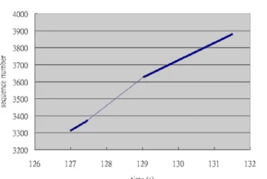
Fig. 6: Sequence numbers of packets that the mobile node receives with speedy handover.

Figure 6 depicts the performance when the speedy handover mechanism is used. The old FA buffers the packets during handover period and forwards them as soon as the new FA knows how to deliver the packets to the mobile node. The mobile node can receive the packets before handover procedure finishes. The handover procedure is complete at about 129.15 second and the mobile receives forwarded packets at about 128.66 second, so we shorten the time that the mobile node can not receive any packets. After

(8)

handover procedure finish the new packets stream toward the mobile node make the packets out of order. It is the cause of the wavy line in Fig. 6.

Fig. 7: Packet lose rate between handover start to forward finish.

By observing the Fig. 7, we can find that the packet loss rate for speedy handover is much lower than that of original structure. The packet loss rates are 55.41% and 1.61% for the original structure and speedy handover respectively. For a multimedia service, low packet loss rate is an important condition for smooth quality.

Fig. 8: Handover time.

Figure 8 shows the time from the start of handover to end of period that the mobile node can not receive any packets. It is clear that speedy handover can shorten the time.

1.4 Section Conclusion

In short, comparing with the original mobile IP mechanism, speedy handover features a fewer number of packet losses and a shorter handover period. The simulation results demonstrate the effectiveness of the proposed scheme. In this chapter, we propose a so-called “discrete scan” scheme and relative auxiliary mechanisms that collect a set of candidates for next-APs and eventually select the next AP for a mobile node before a forthcoming handoff. Moreover, various existed mechanisms may select next AP with different properties of the next-AP candidates, such as the nearest AP, the approached AP, the AP of highest available bandwidth, or their combination.

2. Discrete Scan

2.1 Introduction

In discrete scan, a mobile node, such as a WiFi phone set, will make use of the idle time in pre-handoff duration to sniff its wireless environment to collect a set of next-AP candidates for a forthcoming handoff. A pre-handoff period is initiated with an event that received signal strength (RSS) from current AP is detected to be lower than a preset threshold for a preset period.

(9)

Figure 9 below illustrates the typical scheme for the wireless NIC in the pre-handoff periods. While working in pre-handoff mode, the wireless NIC has to return to working channel to maintain VoIP connection alive with a certain level of QoS. The time between two working periods, that is, the time of sniffing period plus two switching periods, should not be longer than β ms so that the maximum latency allowed by a real time application, α ms, is maintained if the node will get at least two times of transmission within (α−β) ms, as shown in Fig. 9. During working periods, bidirectional traffic transmits between current AP and the mobile node at least once to deliver the traffics generated in previous absence from working channel. By the end of working periods, the mobile node should issue an extra control frame of power save mode (PSM) to notice the current AP to suspend the packets for the mobile node.

Fig. 9: Scheme for wireless NIC in pre-handoff periods.

Fig. 10: Example sniffing scheme in the environment of 3 channels.

To substitute for the function of neighbor graphs, discrete scan must be able to collect a set of next-AP candidates. One of the nature particular to a seamless handoff is that a mobile node must have entered the coverage area of its next AP before a layer-2 handoff is triggered. Therefore, a mobile node can discover the entire set of next-AP candidates by means of sniffing frames transmitted from APs in various channels. An example design for the sniffing scheme is illustrated in Fig. 10. A sniffing period is designated by 20 ms for each interval of 60 ms. Assume that only three channels are deployed in the

Working periods: The periods for Tx/Rx in the working channel (channel 0) Channel 1

Switching periods: The time for wireless NIC to switch channel

Sniffing periods: The periods for sniffing channels (channel 1~10)

Channel 2 Time Channel 0 Channel 0 α 0 1 2 3 4 Beacon 0 1 2 3 4 0 1 2 3 4 0 1 2 3 4 Beacon Beacon 0 1 2 3 4 Beacon 0 1 2 3 4 0 1 2 3 4 0 1 2 3 4

Beacon Beacon Beacon

0 0 Ch-0 Ch-0Ch-0 Ch-0 Ch-2 Ch-1 Ch-0 Ch-0 Ch-0 Ch-2 Ch-1 Ch-2 Ch-1 Ch-1 AP in channel 1

(10)

concerned area. A beacon interval consists of 5 slots, from slot 0 to slot 4, with slot time 20 ms, and two channels which are different from the working channel will be listened in a sequence of sniffed periods. The sniffed channels should be interleaved so that each channel is probed evenly.

The maximal time required for a mobile node to discover all APs through beacons should be taken into account to set the value of δ2, the threshold RSS to start a pre-handoff period. As an example, 20 ms slot of each 60 ms interval is used for sniffing, that is, 1/3 of total run time is shared to sniff for the next-AP candidates in all channels except the working channel. Each scanned channel takes 5 sniffing periods, equal to 100 ms in total, to ensure to discover of all of the next-AP candidates active in the channel. Therefore, it takes (number of channels–1) * 3 * 100 ms to complete the discrete scan scheme on all of channels. With at the most 11 channels in IEEE 802.11b wireless LAN environment, thus, it takes (11-1) * 3 * 100 ms, equal to 3 sec, to complete a full passive scan. Therefore, a pre-handoff period is suggested to be 3 seconds ahead of a layer-2 handoff.

2.2 Mechanisms to select the nearest AP

Discrete scan surpasses the neighbor graph in the ability to select a proper next AP for a mobile node before the handoff starts. Taking the advantage of the information extracted from MAC frame headers that a mobile node listens through its discrete scan scheme; a desired next AP can be determined by the mobile node along with extra supports from existed wireless LAN system. The feature to determine the next AP may take over the function of a neighbor graph with aids of GPS as proposed in [4].

In a conventional handoff schemes, a mobile node determines the nearest AP by the RSS received from beacons or frames sent by APs during the probe phase of a layer-2 handoff. However, it is recognized that the strongest RSS may be not a prefect indicator of the nearest AP because of the effects by multi-paths interference of microwave communications. Nevertheless, the principle of choosing the next AP by indication of RSS is widely implemented in wireless NIC, since no better indicator is available so far. Discrete scan, discovering next-AP candidates through frames or beacons sent by APs, may restrict the capability to select next AP by their RSS. Furthermore, several mechanisms of a new idea with aids of MAC layer information are proposed in this section to compensate the insufficiency of RSS scheme currently supported by physical layer.

By reading MAC layer headers, a mechanism is designed to record the number of stations that can be listened by the mobile node in each channel. A mobile node learns a station with its MAC address in the frame header transmitted from the station.

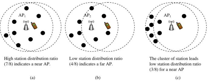
The first proposed mechanism for a mobile node to estimate its distances from candidate APs is named as “station distribution ratio” that is defined as the ratio of the numbers of stations of in the coverage of the mobile node to all of the stations in a BSS. As illustrated in Fig. 11(a) (b), the higher station distribution ratio is a BSS, the nearer is the AP to the mobile node.

Fig. 11: the higher station distribution ratio indicates the nearer AP.

AP1

High station distribution ratio (7/8) indicates a near AP.

(a)

AP2

Low station distribution ratio (4/8) indicates a far AP.

(b)

AP1

The cluster of station leads low station distribution ratio (3/8) for a near AP

(11)

A mobile node can identify a station in its coverage area if the mobile node can receive both a data frame and the corresponding ACK frame in its discrete scan scheme. Similarly, if a mobile node receives only one of a data frame or the corresponding ACK frame, the mobile node infers that the station in the BSS locates out of its coverage. Another good feature that discrete scan surpasses neighbor graphs is its slight penalty if an incorrect AP is selected by the auxiliary mechanisms. A mobile node always locates at the overlapped coverage of all of the next-AP candidates discovered in the discrete scan scheme, therefore, an improper selection among the next-AP candidates will not lead to a failure of a handoff. On the contrary, a mobile node will lose connection if the GPS in a mobile node predicts a neighboring AP that can not reach to the mobile node as the next AP. As illustrated in Fig. 11(c), the cluster of stations in a BSS may lead the station distribution ratio mechanism to an improper selection of the next AP. However, the penalty for a mobile node to handoff to a farer AP may just cause another handoff to occur earlier.

There are some shortcomings of the station distribution ratio mechanism. It will be active only after an AP is discovered because a mobile node infers a station out of its coverage by frames from AP instead of the station. Consequently, the station distribution ratio mechanism requires a certain amount of time to evaluate an AP after it is discovered. Besides, a mobile node needs more extra cache to memorize the MAC addresses of discovered stations to avoid counting a station twice.

To overcome the above drawbacks, the station distribution ratio mechanism is simplified and submitted as the second mechanism for a mobile node to select the nearest AP among candidate APs. The mechanism is named as “station count” because it suggests a mobile node to select an AP of the most number of stations counted by a mobile node in the last sniffing period prior to a handoff. A mobile node with station count mechanism updates the number of stations it found in a BSS in each short sniffing period (e.g., 20 ms) of a discrete scan scheme. Because the mobile node concerns only the stations that locate in its coverage area and transmit at least one frame in a short sniffing period, much less cache memory is needed to keep MAC addresses of discovered stations, and a simple algorithm that collects the frames of various senders to a receiver is sufficient to identify an active station in the coverage. Furthermore, a mobile node starts to sense a BSS before it enters the coverage; therefore the evaluation of a BSS is available with discrete scan once its AP is discovered by the mobile node.

As illustrated in Fig. 12(a), the nearer is the mobile node to an AP, the larger overlapped coverage the mobile node can listen, and consequently the mobile node can discover more active stations in a sniffing period. Unfortunately, the distance between a mobile node and an AP is not a unique factor that affects the station counts. As illustrated in Fig. 12(b), the total number of stations in a BSS is another major factor that affects the station counts in a sniffing period. Due to the imbalance of number of stations in two BSSs, the far AP may result in larger station count than a near one.

(a) (b)

Fig. 12: The station counts in two BSSs.

AP2 Station count of BSS1 = 6 Station count of BSS2 = 4 AP1 AP2 AP1 Station count of BSS1 = 3 Station count of BSS2 = 5

(12)

The third factor that affects the station counts in a sniffing period is the length of a sniffing period. The longer sniffing time results in larger station count until the mobile node discovers all of the stations in its coverage. On the other hand, if the sniffing period is as short as a slot time in DCF wireless environment, the station count is reduced to the probability for one of the stations in the mobile node’s coverage to get a successful transmission in the given timeslot. Since all of the stations in a BSS share a media of limited bandwidth, a BSS of fewer stations has higher probability to transmit a frame in an arbitrary timeslot because of less collisions and smaller contention windows. Hence, a short sniffing period benefits a BSS containing fewer stations.

The length of sniffing periods of discrete scan is properly set to either balance or alleviate the affect of the station counts brought by imbalance of number of stations in various BSSs. There are two major concerns on setting the length of a sniffing period: first, a long sniffing period may eventually eliminate the affect brought by imbalanced number of stations. Second, a short sniffing time results in insufficient station counts to have creditable selection among the candidate APs.

In the following, we will elaborate the way to determine an appropriate length of a sniffing period. The model proposed by G. Bianchi [5] is employed for the analysis of DCF wireless LAN environment. 2.3 Setting of a sniffing period

As described before and illustrated in Fig. 12(a) (b), two factors control the station count of a BSS, distances between the mobile node and the AP and number of stations in the BSS. Intuitively, we have

A A r s

E( )≈ ⋅ '/ ₍₁₎

where E(s) denotes the expected value for s, and s denotes the station count of a BSS in a sniffing period that is represented by Tsniff ; r is a new term called as “number of transient stations”, that is defined as the number of stations which at least send one frame in given sniffing time (Tsniff) in a BSS; and A’ denotes the overlapped coverage of a BSS and the mobile node, and A denotes the coverage area of BSS.

Let τ denote the probability that a station transmits in an arbitrary slot time, and p denotes the probability that a transmitted packet encounters a collision. By [5], in a BSS of DCF wireless environment, there are

) ) 2 ( 1 ( ) 1 )( 2 1 ( ) 2 1 ( 2 m p pW W p p − + + − − = τ (2) 1 ) 1 ( 1− − − = n p τ ₍₃₎

where, n is the number of stations in a BSS

W is the minimal contention window in DCF.

m is the integer such that 2mW presents the maximal contention window in DCF.

For a given n, τ and p are derived from (2) and (3). Thus, the average number of frames transmitted within one timeslot would be τ∗n.

Let Ptr denote the probability that at least one frame is sent in a considered timeslot. There are n stations and each station transmits a frame with probability τ, therefore,

n tr

P =1−(1−τ) (4)

Let Ps denote the probability of a successful transmission in a considered timeslot, i.e., the probability that exactly one station transmits on the channel, under the condition of the fact that at least one station transmits. It has,

n n tr n s n P n P ) 1 ( 1 ) 1 ( ) 1 ( 1 1 τ τ τ τ τ − − − = − = − − (5) Let σ be a slot time in the condition of idle media. Ts denotes the length of a slot time in the

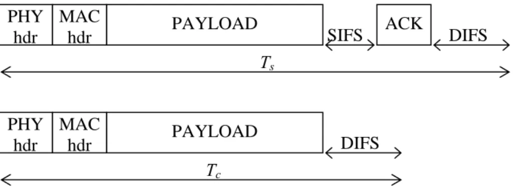
condition of a successful transmission and Tc denotes the length of a slot time in the condition of a transmission with collision, as defined in Fig. 13.

δ δ + + + + + + +

=PHYhdr MAChdr E P SIFS ACK DIFS

T_s [ ] (6) δ + + + +

=PHYhdr MAChdr E P DIFS

(13)

where, δ stands for the propagation delay, E[P] is the average length of packet payload and E[P*] is the length of the longest packet payload involved in a collision.

Fig. 13: Definition of Ts and Tc, slot time of transmission with success and collision.

The average length of a slot time, denoted by Tav, is readily obtained by considering that, with probability (1-Ptr), the slot is null of transmission; with probability Ptr Ps, the slot contains a successful transmission, and with probability Ptr(1-Ptr), the slot contains a collision. Hence,

c s tr s s tr tr av P P PT P P T T =(1− )σ + + (1− ) (8)

Let m denote the total number of frames sent by n stations within Tsniff. It is estimated in average as,

av sniff T T n m= τ* / (9) Parameters Values PLCP preamble & header 192.0 μs

MAC header 20.4 μs

Slot time 20 μs

SIFS 10 μs

DIFS 50 μs

ACK 10.2 μs + PLCP preamble & header

CWmin 32

CWmax 1023

Maximal Packet payload 2312 bytes Channel bit rate 11 Mbps

Table 1 Parameters for IEEE 802.11b wireless LAN.

Assume that n stations transmit m frames randomly. The number of transient stations, r, is the number of stations that send at the least one of m frames in Tsniff. Thus, r is derived as follows:

PHY hdr PAYLOAD SIFS MAC hdr ACK Ts DIFS PHY hdr PAYLOAD MAC hdr Tc DIFS

(14)

( ) ( )

∑

= = ⋅ ⋅ ⋅ = _n k n k m,k S n,k P m,k S n,k P k r 1 1 (10)

where, S(m,n) denotes the Stirling number of the second kind, as,

( )

_∑

( )

= = n k m n n-k k _n-k -n m,n S 0 1 ! 1 (11) and P(n,k) denotes the permutation number as,

)! ( ! ) , ( k n n k n P − = (12)

Note that m in (9) is not an integer but m in (10) and (11) is restricted to an integer. Interpolation will be used in the numerical approach below.

With equations (2)~(12) and parameters listed in Table 1 for an IEEE 802.11b wireless LAN, the relations of transient number of station(r) v.s. number of station(n) of various Tsniff values are demonstrated in Fig. 14.

Number of transient stations (r) v.s number of stations for different Tsniff values

0 5 10 15 20 0 5 10 15 20 25 30 Number of stations (n) in BSS

number of transient stations

(r ) ₁₅ 20 25 30 40

Fig. 14: Number of transient stations (r) vs number of stations (n) for different Tsniff values.

By reviewing equation (1), a station count (s) linearly depends on overlapped area (A’) and transient number of station(r) with respect to a Tsniff. Since it is desired that a station count to indicates overlapped

area (A’) rather than being disturbed by the imbalance of numbers of stations in different BSSs, an appropriate sniffing period (Tsniff) should be set so that the number of transient stations (r) behaves insensitively to variation of the number of stations (n).

Figure 14 shows the fact that a shorter sniffing period (Tsniff) responds to a number of transient stations (r) less insensitive to variation of number of stations (n). However, as described in the previous section, a sniffing period should be long enough to make station counts big enough for a creditable

(15)

selection. In this project, we recommend that in a BSS of fewer stations (such as n = 6), number of transient stations (r) should be 80 % of number of stations (n), i.e., r > 4.8 as n = 6. By the curves in Fig. 14, a sniffing period Tsniff is eventually chosen as 20 ms because the curve of Tsniff = 20 ms shows that its

transient stations equal to 5 at n = 6. As n = 24, the number of stations increases by 4 times, the number of transient stations (r) is approximately equal to 10, increased by only 2 times. The numerical result shows that the variation of number of stations in a BSS reflects only half of numbers of transient station by setting a sniffing period as 20 ms. Although there is no proper sniffing period to make number of transient stations independent of number of station, however, the effect brought by imbalance of number of stations has been significantly mitigated by 50%

2. 4 Performance of Station Count Mechanism

E(s), the expected value of the station count with respect to a given Tsniff, is approximately equal to

r*A’/A as described in (1), while collisions within overlapped area, A’, is neglected. In this section, the

collisions are taken into consideration for a more accurate formula to estimate E(s).

The average number of stations lies in the overlapped coverage that is estimated by area proportion, so that n’ = n*A’/A. Let m’ denote the total frames sent by either one of n’ stations (no collision with any frame sent by one of n’ stations) in Tsniff, then m’ is estimated in (13), where τ is given in (2) and m is

given in (9) n n m T T n m n av sniff n / ' ) 1 ( / ) 1 ( ' '= τ −τ '−1⋅ = ⋅ −τ '−1⋅ (13)

Same as the process to estimate the number of transient stations, assuming that n’ stations transmit

m’ frames randomly and let μ denote the reformed station count, the number of stations that sends at least one of m’ frames in Tsniff. Thus, μ can be derived using (14) below.

( ) (

)

( ) (

)

∑

= = ′ ⋅ ′ ′ ⋅ ′ ⋅ = _n k n k ,k m S ,k n P ,k m S ,k n P k 1 1 μ (14)

where, S(m,n) denotes the Stirling number of the second kind that is defined in (11), and P(n,k) denotes permutation number that is defined in (12)

Note that m’ in (13) may not be an integer and m’ in (14) is restricted to an integer. Interpolation is used for numerical approach below.

Let Si denote the random variable of station count in a sniffing period Tsniff for ith channel. It is

reasonably assumed that Si features Poisson distribution and μi derived in (14), an estimation of reformed

station count for ith channel, should be the average of random variable Si, i.e., μi = E(si).

Fig. 15: Scenario for performance estimation.

The scenario to display the performance of station count mechanism is illustrated in Fig. 15. It 14

=

n2 n1 = 9

(16)

assumes that a mobile node with discrete scan scheme roams in the overlapped coverage of two next-AP candidates. The current AP is not shown in Fig. 15, for its location will be irrelevant to performance of the station count mechanism. The mobile node selects one of two next-AP candidates, AP1 and AP2,

according to their station counts derived in the last two sniffing periods of the discrete scan. Let h denote the hit ratio, the probability that the mobile node selects the nearest AP with the indication of larger station count as its next AP. Therefore, the mathematical definition for h in the case of two candidates is given in (15). ) | ( 2 1 ) | (s₁ s₂ d₁ d₂ p s₁ s₂ d₁ d₂ p h= > < + = < (15)

where p(…|…) denotes the conditioned probability; si denotes the station count in Tsniff of ith channel; and di denotes the distance between the mobile node and the AP in channel i (denoted by APi).

The average station count in each channel, μ1 and μ2, is estimated by (14) with given n1, n2, d1, d2, Tsniff as wells as parameters for DCF wireless environment (listed in Table 1). Since S1 and S2 are in

Poisson distribution of mean values E(s1) = μ1 and E(s2) = μ2, the hit ratio h, defined in (15) is estimated

by, )] ( 2 1 ) ( [ ) ( 2 1 2 1 k p s k p s k s p h k = + < ⋅ = =

∑

∞ = ] ) ! 2 ! ( ! [ 1 0 2 2 1 1 ) ( ₁ ₂

∑

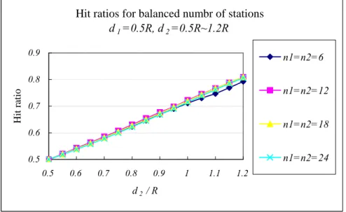
− = ∞ = + − ₊ = k l k l k k k l k e μ μ μ μ μ (16)

Hit ratios are demonstrated for the conditions that the mobile node locates at the place d1 = 0.5R and d2 varies from 0.5R to 1.2R, where R denotes the radius of coverage of BSSs and the mobile node. Tsniff is

set as 20 ms. In the first case, it demonstrates how the distances between the mobile node and APs affect the hit ratio by setting the same number of stations in BSSs to ignore effects of the imbalance of numbers of stations in BSSs. In Fig. 16, the curves are given for hit ratios (h) with respect to various distances from AP2 (d2) in cases of n1 = n2 = 6, 12, 18 and 24.

Hit ratios for balanced numbr of stations

d1=0.5R, d2=0.5R~1.2R 0.5 0.6 0.7 0.8 0.9 0.5 0.6 0.7 0.8 0.9 1 1.1 1.2 d2 / R Hit r atio n1=n2=6 n1=n2=12 n1=n2=18 n1=n2=24

Fig. 16: Hit ratios vs distances in balanced number of stations.

Fig. 16 shows that the hit ratios increase almost linearly with the increase of distance between the mobile node and the competing AP (d2), while the distance from the mobile node to the selected AP (d1)

is set fixed and the effect of imbalanced number of stations are ignored, i.e., n1 = n2. From observation of Fig. 16, it indicates that the number of stations, if they are evenly distributed, will be almost independent to the hit ratios.

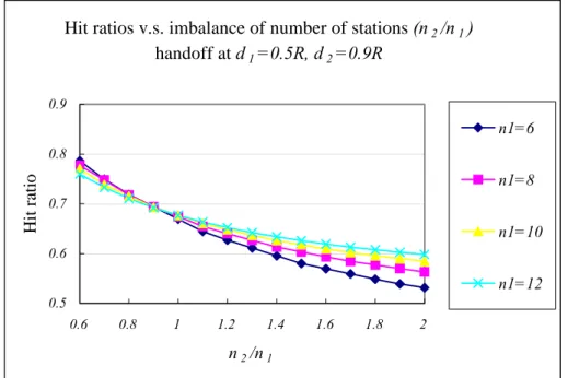
In the second case, we investigate the affect of imbalanced number of stations on the hit ratios. The mobile node keeps its location at the place d1 = 0.5R and d2 = 0.9R. Four cases of variation of number of

(17)

n2, varies from 0.6 to 2 times of n1 and the corresponding hit ratios are computed and presented in curves,

as shown in Fig. 17.

Hit ratios v.s. imbalance of number of stations (n₂/n₁) handoff at d₁=0.5R, d₂=0.9R 0.5 0.6 0.7 0.8 0.9 0.6 0.8 1 1.2 1.4 1.6 1.8 2 n2/n1 Hit ratio n1=6 n1=8 n1=10 n1=12

Fig. 17: Variation of hit ratios with imbalance of number of stations.

Observe the curves in Fig. 16, the imbalance of number of stations do affect the hit ratios. In the neutral number of stations, i.e., n2 = n1, the hit ratios for all of the four cases are about 0.68. With the increase of imbalance, i.e., increasing n2 / n1, the hit ratios decrease with moderate slopes. As to the most imbalanced number of stations, i.e., case of n2 = 2n1, the hit ratios drop to about 0.55~0.6. The hit ratio decreases by less than 20% due to the number of stations of competing BSS increases up to double. In addition, it is more sensitive to the disturbance of imbalance in number of stations in case of fewer stations in the selected BSS (BBS1). From Fig. 17, in the case that most of stations are in selected BSS

(i.e., n1 = 12), the hit ratio drops to about 10% (from 0.68 to 0.6) with the increase of imbalance (n2 / n1) from 1.0 to 2.0. On the other hand, the hit ratio drops to about 20% (from 0.68 to 0.55) in case that there are fewest stations in the selected BSS (n1 = 6).

2.5 Select best next AP instead of the nearest AP

The traditional handoff scheme that determines the next AP to handoff to by the RSS (receive signal strength) received from the responding AP in the probe phase of a layer-2 handoff. The strongest RSS is recognized as an indicator of the nearest AP, because shorter distance is subject to stronger signal strength. Same as RSS, the mechanisms presented before help a roaming node select the nearest AP by the link-layer information obtained in discrete scans. However, the nearest AP may not be the best next AP to handoff to. The available bandwidth that the next BSS can offer is one of the most concerned items especially for a mobile node in real time application, such as a WiFi VoIP connection. Besides, an AP that the mobile node is approaching to may be a better selection of the next AP than those from which the mobile node is moving away, even the latter ones are detected with stronger RSS.

Discrete scan schemes may be used to detect characteristics of a BSS by the collection of frames transmitted in a BSS in advance to a handoff. With information from sniffed frames, a mobile node may select the best next AP rather than the possible nearest AP with the indication of RSS in a traditional handoff scheme.

The available bandwidth and access delay of a BSS can be detected by the average NAV values in the frames collected in discrete scans. The relations between the NAV values and available bandwidth as well as access delay in a BSS are inferred to be linearly dependent in [6] with both mathematical analysis and simulation. A mobile node with discrete scan will be able to estimate the available bandwidths and access delays of the next-BSS candidates by NAVs collected in its sniffing periods and determine the best next AP when a handoff is triggered.

(18)

Furthermore, the trends of station counts along certain sniffing periods for a BSS may be used to indicate whether the sniffing node is approaching to an AP or not. For the AP that a mobile node is approaching to, the station counts shall be in an increasing trend because the mobile node can listen to more stations when it is closing to the AP. To select an approaching AP rather than the nearest AP may alleviate the frequent handoffs in the hot spot where the cell of a BSS may be relatively small.

The attributes that assist a mobile node to determine its next AP in handoffs may be integrated as an objective function with appropriate weights assigned to all of the indicators. With combinational considerations on receive signal strength, distances, approaches, as well as available bandwidth, the objective function for a mobile node to evaluate ith BSS can be written as,

i i

i w RSS w STA count w STA count w NAV

F = 1( ) + 2( _ ) + 3(Δ _ ) + 4( ) (17)

2.6 Impact on service QoS

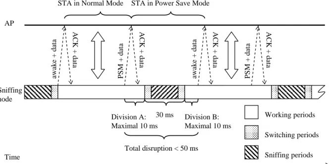
The most concerns on the discrete scan schemes may attribute to its impact on the service QoS in a pre-handoff period, since part of service time is taken out to sniff on other channels. During the sniffing periods, the service of working channel will be interrupted and this causes a certain level of access delay. Furthermore, because of absence from working channel, the frames that the current AP sends to the mobile node during a sniffing period will be lost. However, as described in chapter 1, the applications that require seamless handoffs are mostly of relative low bit rate as compared with that a wireless NIC can offer. Therefore, with proper design, a mobile node may use a large portion of idle time of wireless NIC for discrete scan; thus, to minimize the impacts caused by discrete scan. In this section, a VoIP connection which runs with bidirectional 64 kbps constant bit rate in an IEEE 802.11b wireless LAN of 11Mbps are taken as an example for the discussion on the impact on service QoS brought by discrete scan scheme.

Besides a sniffing period of 20 ms, the channel switch time of a wireless NIC contributes to disruption of service from working channel as a major part. In this project, the channel switch time is assumed as 5 ms as in [3]. To complete a sniffing period in discrete scan scheme, it needs to do twice for switching channels, one for leaving from the working channel and the other for returning back. Therefore, it brings an absence period of at least 30 ms from the working channel to execute once of discrete scan.

A disruption of 50 ms may be the upper bound for a seamless handoff to tolerate. The principle of the discrete scan is to decompose time for the probe phase of a layer-2 handoff into a pre-handoff period, such that no more than 50 ms disruptions are induced during pre-handoff and handoff procedures.

Fig. 18: Total disruptions induced with a discrete scan.

Total disruption < 50 ms STA in Power Save Mode STA in Normal Mode

awake + data PSM + data

ACK + data

awake + data PSM + data

ACK + data ACK + data Division B: Maximal 10 ms Division A: Maximal 10 ms 30 ms Sniffing node AP Time Working periods Switching periods Sniffing periods

(19)

Nowadays, the QoS issue for real time applications in IEEE 802.11 wireless LAN is still widely discussed. In most of infrastructure wireless LAN environment, downlink traffics from AP to all the stations is much heavier than the uplink traffic from a single station to the AP. However, the transmission opportunity of AP is same as that of a single station, thus the downlink flow shares the bandwidth with those uplink flows from all stations. In other words, the shared bandwidth of the downlink transmission from AP to arbitrary one of stations will be only 1/n of the bandwidth of the uplink transmission to AP, where n denotes number of stations in a BSS. Because of the asymmetric nature between uplink and downlink transmission, a real time application with symmetric bidirectional transmission may suffer from severely degraded QoS of downlink flow when the number of stations in a BSS increases.

To address the QoS problems caused by asymmetric transmission opportunity for a specific station with symmetric bidirectional traffics, piggyback schemes [7] in IEEE 802.11 standard suppose to forward the downlink traffic as an attachment to a positive ACK frames from AP to stations. With piggyback schemes, the QoS issue of asymmetric transmission opportunity is therefore eliminated. The QoS provisioning to symmetric bidirectional service then is considered as the QoS to the uplink flow of the concerned station.

As illustrated in Fig. 18, the total disruption caused by discrete scans should be computed from the transmission of the last frames before wireless NIC switches to a sniffing channel until the transmission of the first frame after wireless NIC returns back to working channel. The duration for a wireless NIC absent from working channel is 30 ms for each sniffing period and the total disruption has to be kept less than 50 ms, therefore, the two sentinel frames, defined as the last frame before channel switch and the first frame after the return, have to be transmitted within the periods of 20 ms in total.

The rest of 20 ms for sentinel frames is divided into division A and B (shown in Fig. 18). A mobile node converses a disruption caused by a sniffing period less than 50 ms, if it transmits the first sentinel frame in division A and the second sentinel frame in division B. In the case the first sentinel frame fails to be transmitted with the division A period, the piece of sniffing period should be slipped until next cycle. As the first sentinel frame has been sent, the total disruption brought by the sniffing period is equal to 50 ms + (time to the 2nd sentinel frame – division B) – time to the 1st sentinel frame. To keep the disruption less than 50 ms in all case, a mobile node should promise to send the second sentinel frame by the end of division B.

In the simplest design, each sentinel frame for a sniffing period evenly shares 10 ms as its maximal allowable time for the mobile node to transmit a sentinel frame successfully. Thus we have division A = division B = 10 ms. Therefore, the capability that a mobile node guarantees to send one frame successful in 10 ms decides whether the disruptions brought by a discrete scan can be conserved within 50 ms. In this section, the analytical model of DCF wireless environment presented before is employed to estimate the probability for a mobile node in IEEE 802.11b wireless LAN to transmit one frame successfully within 10 ms.

With known transmitting probability in a slot time, τ, given in (2) and the average length of a slot time, Tav, given in (8), the average number of frames that the mobile node could transmit within 10 ms

can be derived as,

av

T ms

m"=τ*10 / (18)

Taking the probability that a transmitted packet encounters a collision, p, given in (5), the probability that at least one of m” frames transmitted without a collision is estimated by,

"

1 m

sentinel p

p = − (19)

Numerical results of (19) with the parameters listed in Table 1 for BSSs of 11 Mbps as well as 54 Mbps are given in Fig. 19. When number of stations increases up to 6, the probability for a station to transmit a frame without collisions within 10 ms drops to lower than 80% in an IEEE 802.11b 11Mbps wireless LAN, therefore, more than 20% of sniffing periods will be slipped. It is inferred about 20% of disruptions brought by sniffing periods to be longer than 50 ms when the BSS supports more than 6 stations simultaneously. Figure 19 shows that even bit rate of the BSS increases up to 54 Mbps, stations that the BSS can support based on the same criteria increases to only 12. Note that, as shown in Fig. 16 and 17, the station count mechanism proposed before assumes a number of stations greater 6 to promise

(20)

creditable selections. It consequently concludes that the discrete scan with station count mechanism proposed before will not work together very well in the DCF environments. However, instead of DCF, an IEEE 802.11e EDCA wireless environment grants VoIP traffic with high priority of transmission and promise it to send one frame within 10 ms at a much higher probability even with more than 10 stations in the BSS.

How discrete scan and station count mechanism proposed in this project can work together in an IEEE 802.11e ECDA wireless environment will be elaborated with results of ns-2 simulation. To set a proper length for a sniff period, the performance to hit the desired nearest AP as well as probabilities that the disruptions for sniffing periods converge within 50 ms will be demonstrated.

Probability for a staion to transmit a frame within 10 ms in IEEE 802.11b DCF 11Mbps environment 0 0.2 0.4 0.6 0.8 1 0 10 20 30 Number of station (n) in BSS P robability 11Mbps 54Mbps

Fig. 19: Probability to transmit a frame in 10 ms vs number of stations in a BSS.

2.7 Performance evaluation AP2 AP1 11Mpbs 11Mpbs 100Mpbs 2μs FTP Server or VoIP agent Gateway 100Mpbs 20ms 100Mpbs 2μs Internet 11Mpbs 11Mpbs 100Mpbs 2μs 100Mpbs 2μs FTP Server or VoIP agent Gateway

(21)

Fig. 20: Simulation configuration.

We evaluate the performance for discrete scan schemes in IEEE 802.11e EDCA wireless LAN environment by means of simulations. We discuss the major concern, the impact of service QoS, while a mobile node applies discrete scan scheme in EDCA wireless LAN. Attributing to the high transmission priority of VoIP traffic, the impact on QoS caused by discrete scan schemes in EDCA environment is shown within the tolerable limits according to the simulation results.

Simulation Environment

We use NS-2 (version 2.28) tool [8] with 802.11e tkn EDCA module [9], we neglect high-level management functionality such as beacon frames, association and authentication frame exchanges. In all scenarios, the network topology of the simulations is shown in Fig. 20. Each of wireless stations either runs bidirectional VoIP traffic or TCP traffic with its corresponding wired station playing as either a VoIP device or FTP server. VoIP traffic, with format of G.711 codec, 160 bytes payload and 20ms intervals are used as real-time traffic, and FTP traffic of 1,500 bytes payload are used to simulate the best effort traffic. Table 2 shows the default parameter values of EDCA in the simulations. Besides, 10% of wireless packet error rate is set to simulate the transmission in the real environment. Furthermore, for the sake of distributed arrival time of VoIP packets, each of VoIP traffic is initiated at a randomly selected time from sec 5th to 6th sec. The observed scan periods for each channel are taken from 10th sec to 20th second, so that the traffics in BSSs are assumed in steady state. The simulation ends at 25th second.

With various random seeds for each run, uniformly distributed random function which is built-in in ns-2 programs generates the locations of the mobile nodes in both BSSs. The normal combination of traffics is assumed that 70% of nodes run in TCP traffic and 30% of nodes play as VoIP phones. However, BSSs of all TCP nodes and all VoIP nodes are running in order to discuss the affects by various traffics in a BSS.

AC PF AIFS CW_MIN CW_MAX TXOP Limit (s)

voice 2 2 7 15 0.003008

best effort 2 3 31 1023 0 Table 2: Default values of parameters for original EDCA.

Station Count Mechanism in EDCA Environment

As discussed before, by properly selecting a sniffing time may eliminate affects on the hit ratio in selecting the nearest AP caused by imbalance of number of stations between the next-BSS candidates. The number of transient stations (denoted by r) is defined as the average number of stations that transmit at least once within a sniffing period (denoted by Tsniff) in a BSS. A proper sniffing time shall meet two

conditions: first, make the number of transient stations varies as insensitively as possible with the variation of number of station in a BSS. Usually the less the sniff time is, the better the attribute will be. Second, the sniff time shall be long enough for a mobile node to discover the next-AP candidates as well as to collect enough frames to infer a creditable selection result.

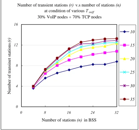
In Fig. 21, it shows the curves for transient number of stations v.s. various numbers of stations for several given values of sniffing periods in an EDCA BSS of 70% TCP and 30% VoIP nodes. The curves in Fig. 21 show that number of transient stations is fairly insensitive to number of stations as the number of stations in a BSS is large (e.g. n > 12). When the number of stations in a BSS is small (e.g. n < 6), the

(22)

number of transient stations increases at a rate about a half of increasing rate of number of stations. The selection results are still disturbed by the imbalance of number of stations, especially when number of stations is small in both EDCA and DCF wireless environment. However, the effect is reduced to at least half of the difference of number of stations by setting a sniff period to 15 ~ 20 ms.

Number of transient stations (r) v.s number of stations (n) at condition of various T_sniff

30% VoIP nodes + 70% TCP nodes

0 4 8 12 16 0 8 16 24 32 Number of stations (n) in BSS N u mber of t rans inet s tat ions (r ) 10 15 20 25 30 35

Fig. 21: Number of transient stations v.s. number of stations in EDCA of 70% TCP and 30% VoIP nodes.

Numer of transient stations (r) v.s Number of stations (n) at condition of various Tsniff

100 % TCP traffics 0 4 8 12 16 0 8 16 24 32 Number of stations (n)

Number of transinet stations

(r) 10 15 20 25 30 35

(23)

Fig. 22: Number of transient stations v.s. number of stations in EDCA with 100% TCP nodes.

Figure 22 shows the curves with the same condition as those in Fig. 21 except that EDCA BSS features 100% of TCP nodes. With mostly the same trends as that in Fig. 21, the curves in Fig. 22 shows less steep slope and apparently lower values of number of transient stations than those in Fig. 21. It is inferred that most VoIP nodes are discovered and contribute to number of transient stations because of the attributes of high transmission priority and short packet length of VoIP traffic. Consequently, the station count mechanism tends to select a BSS with more VoIP nodes as the next AP to handoff to if the other control factors, such as distances and number of stations are neutral between BSSs.

Performance of Station Count Mechanism in EDCA Environment

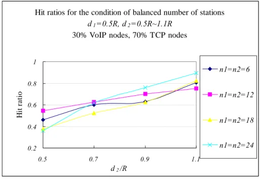
Figure 23 shows that the hit ratios with respect to various distances (d2 = 0.5R ~ 1.1R) from the

competing APs. The selected AP locates at a fixed distance (d1 = 0.5R) from the mobile node. The

number of stations in both BSSs are set to the same set of numbers (n1 = n2 = 6, 12, 18, 24) to minimize

the effects caused by imbalanced number of stations. Both next-BSS candidates work as EDCA wireless LANs consisting of 70% TCP and 30% VoIP nodes.

As the same situation as those in DCF environment (shown in Fig. 16), the hit ratios increase linearly with the increase of the distance between the mobile node and the competing APs, d2, while d1 is

fixed and number of stations are evenly distributed. It is inferred that the distances between a mobile node and next-AP candidates affect the hit ratios to select the nearest AP regardless the type of wireless LANs, with the assumption of evenly distributed stations. Consequently, it concludes that the station count mechanism works under EDCA as well as under DCF.

Figure 24 shows the hit ratios with the same as condition in Fig. 23 except that the EDCA BSS consists of 100% TCP nodes. Compared with that in Fig. 23 and Fig. 16, it is inferred again that the distance dominates the hit ratios linearly. However, the deviation among curves of numbers of stations (n1 and n2) is apparently larger than that in Fig. 24. As described in previous section, a mobile node will

discover most of the VoIP nodes in its coverage; therefore, these VoIP nodes contribute to the station count. The curves in Fig. 24 display a trend much similar to those in Fig. 16 because EDCA is reduced to DCF if only best effort access category (AC) exist in an EDCA BSS.

Hit ratios for the condition of balanced number of stations

d1=0.5R, d2=0.5R~1.1R

30% VoIP nodes, 70% TCP nodes

0.2 0.4 0.6 0.8 1 0.5 0.7 0.9 1.1 d2/R H it ra ti o n1=n2=6 n1=n2=12 n1=n2=18 n1=n2=24

Fig. 23: Hit ratios v.s. distances in balanced number of stations in EDCA WLAN of 30% VoIP nodes and 70% TCP nodes.

Furthermore, with existence of VoIP nodes in EDCA, small portion (e.g. 30%) of VoIP nodes dominate the selection of the next AP. The station count mechanism may select a BSS of more VoIP

(24)

nodes rather than the nearest one.

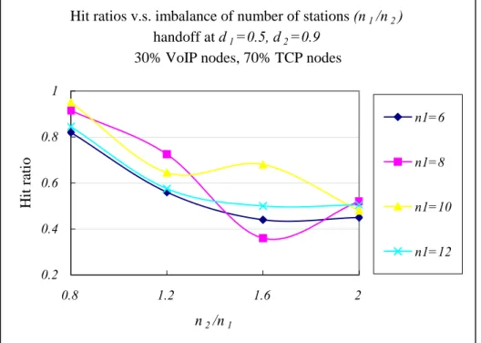
Figure 25 shows the effects on hit ratios caused imbalance number of stations in an EDCA BSS of 70% TCP nodes and 30% VoIP nodes. Same as those in Fig. 17, the mobile node locates at the place d1 = 0.5R and d2 = 0.9R, the number of stations of BSS1, n1 = 6, 8, 10 and 12, and the imbalance of number of

stations of BSS2, n2/n1 varying from 0.6 to 2.

Hit ratios for the condition of balanced number of stations

d1=0.5R, d2=0.5R~1.1R 100% TCP traffic 0.2 0.4 0.6 0.8 1 0.5 0.7 0.9 1.1 d2/R H it ra tio n1=n2=6 n1=n2=12 n1=n2=18 n1=n2=24

Fig. 24: Hit ratios v.s. distances in balanced number of stations in EDCA WLAN of 100% TCP traffic.

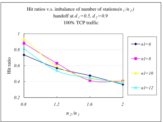
Figure 26 shows the hit ratios of the same settings in Fig. 25 except that the EDCA has only TCP nodes. Figure 25 and Fig. 26 show the interference of imbalanced number of stations in the next EDCA BSSs candidates on the hit ratios of station count mechanism are of the same averages and trends, except that the curves in Fig. 25 are of larger deviation from their average values. As interpreted above, the existence of VoIP nodes contribute the deviation to the curves in Fig. 25, because few VoIP nodes dominate the selection results.

Hit ratios v.s. imbalance of number of stations (n1/n2)

handoff at d1=0.5, d2=0.9

30% VoIP nodes, 70% TCP nodes

0.2 0.4 0.6 0.8 1 0.8 1.2 1.6 2 n2/n1 H it ratio n1=6 n1=8 n1=10 n1=12

(25)

in EDCA of 30% VoIP nodes and 70% TCP nodes.

Hit ratios v.s. imbalance of number of stations(n1/n2)

handoff at d1=0.5, d2=0.9 100% TCP traffic 0.2 0.4 0.6 0.8 1 0.8 1.2 1.6 2 n2/n1 H it ratio n1=6 n1=8 n1=10 n1=12

Fig. 26: Hit ratios v.s. imbalance of number of stations in EDCA of 100% TCP traffic.

With the discussion above, the existence of VoIP nodes may contribute a negative factor for station count mechanism to select the nearest AP. Generally speaking, VoIP packets are generated in an interval of 20 ms and transmitted within bounded jitter to meet real-time requirement. Since a sniffing period is suggested to be as long as 20 ms, it implies that all VoIP nodes transmit a frame each sniffing period. Therefore, the number of VoIP nodes is included in the number of transient stations in an EDCA BSS, then, it causes station count mechanism intending to select a BSS of more VoIP nodes rather than the nearest one.

It is still not yet to comment as a good or bad feature for station count mechanism to select an AP of more VoIP nodes in its BSS rather than the nearest one. However, the feature can be designed as an option because of the simplicity to filter out the frames from VoIP nodes by the specific characteristic of its packets. As the frames for VoIP traffic are ignored in the sniffing periods, the performance of the station count mechanism in EDCA environment reforms to be similar to that in DCF and with less deviation from the mean values, as shown in Fig. 24 and Fig. 26.

Impact on Service QoS in EDCA Environment

Referring to the discussion before and the scheme shown in Fig. 18, to conserve the seamless requirement and protect services from a disruption of more than 50ms, a VoIP node with discrete scan scheme shall ensure to transmit one frame successfully within 10 ms before and after a sniffing period. In an EDCA wireless LAN, VoIP traffic is granted with the highest transmission priority, therefore, the contentions for a VoIP flow in EDCA wireless LAN to get medium are much less intense than those in DCF one. In Fig. 27, it shows the probabilities for a VoIP node to send at least one frame in 10 ms with respect to the number of stations in an EDCA wireless LAN with 11Mbps rates. Three cases for further discussion are assumed: first, 10% of transmission error in the wireless environment and 100% of stations in a BSS are VoIP nodes; second, 10% of transmission error in the wireless environment and normal traffic combination (30% VoIP nodes and 70% TCP nodes) for stations in a BSS; third, in the error free wireless environment and 100% of VoIP nodes for all stations in a BSS.

The curves in Fig. 27 display that the probabilities for a VoIP node to send a frame in 10 ms in the EDCA environment are more dependent on the air transmission error rather than on the number of

(26)

stations in its BSS. In worst condition such that more than 20 VoIP running simultaneously in an EDCA BSS with 10% transmission error, the success probability to send a frame in 10 ms is still kept about 85%. Therefore, the disruption caused by a sniffing period for discrete scan will be maintained within 50 ms with a probability more than 85%. As compared with those for DCF environment, it concludes that the discrete scan schemes proposed in this project are much applicable for a VoIP node in EDCA wireless environment than in DCF one.

Probability for a VoIP node transmitting a frame within 10 ms in IEEE 802.11e EDCA 11Mbps wireless LAN environment

0.7 0.8 0.9 1 0 10 20 30 Number of stations (n) P ro b ab ility 10% error, 100% VoIP 10% error, 30% VoIP Error Free, 100% VoIP

Fig. 27: Probability to send a frame in 10 ms v.s. number of stations in 11 Mbps EDCA wireless LAN.

2.8 Section conclusion

Compared with neighbor graphs, discrete scan scheme provides a set of next-AP candidates as a subset of neighboring APs. With the help of proposed auxiliary mechanisms, discrete scan selects an appropriate next AP for a mobile node to handoff to, taking the place of the function of a neighbor graphs with aids of topological information by GPS system proposed in [4].

As a cost, discrete scan scheme contributes an impact to service QoS received by the mobile node in a “pre-handoff” period that is defined as the duration from initiating the discrete scan scheme to the moment when a handoff is initiated. However, taking the advantages of high transmission priority and relative low bit rate for a VoIP connection in EDCA wireless LANs, the degradation may be limited to a degree that the users may tolerate or even may ignore. Estimation on the QoS degradation with analytical approach and simulation results presented in this and next chapter shows that the disruptions caused by discrete scan are bounded to 50 ms based on certain practical assumption.

3. Two-stage Authentication

3.1 AAA/Mobile IP

We propose a two-stage authentication scheme such as transient authentication and user (re) authentication mechanism. We use AAA/Mobile IP to authenticate a MN and get the certificate from MAP during registration simultaneously. This certificate signed by MAP can be used in the same MAP domain to get the different local certificate from different access routers for passing the filtering rule of MN. Figure 23 shows the authentication message flow in AAA/Mobile IP as shown in Figure 28. A mobile node sends its NAI in registration request and AAAF forwards registration message with