Single-Machine Scheduling to Minimize Total Completion Time and Tardiness with Two Competing Agents

(1)

Research Article

Single-Machine Scheduling to Minimize Total Completion

Time and Tardiness with Two Competing Agents

Wen-Chiung Lee,

1

Yau-Ren Shiau,

2

Yu-Hsiang Chung,

3

and Lawson Ding

1

1_{Department of Statistics, Feng Chia University, Taichung, Taiwan}

2_{Department of Industrial Engineering and System Management, Feng Chia University, Taichung, Taiwan} 3_{Department of Industrial & Engineering Management, National Chiao Tung University, Hsinchu, Taiwan}

Correspondence should be addressed to Wen-Chiung Lee; [email protected] Received 25 November 2013; Accepted 12 December 2013; Published 19 January 2014 Academic Editors: F. R. B. Cruz and A. Sede˜no-noda

Copyright © 2014 Wen-Chiung Lee et al. This is an open access article distributed under the Creative Commons Attribution License, which permits unrestricted use, distribution, and reproduction in any medium, provided the original work is properly cited.

We consider a single-machine two-agent problem where the objective is to minimize a weighted combination of the total completion time and the total tardiness of jobs from the first agent given that no tardy jobs are allowed for the second agent. A branch-and-bound algorithm is developed to derive the optimal sequence and two simulated annealing heuristic algorithms are proposed to search for the near-optimal solutions. Computational experiments are also conducted to evaluate the proposed branch-and-bound and simulated annealing algorithms.

1. Introduction

In traditional scheduling, there is a common goal to minimize

for all the jobs [1–4]. In contrast to that, there is a growing

interest in multiagent scheduling problems where jobs are from several customers who have different goals to pursue.

For instance, Peha [5] gave the telecommunication service

examples where various types of packets and service compete for the use of a commercial satellite, and the problem is to satisfy the service requirements of individual agents to transfer voice, image, and text files for their clients. Brewer

and Plott [6] gave a transportation example where the agents

own transportation resources and compete for the usage of

the infrastructures. Kubzin and Strusevich [7] presented an

example that maintenance operations complete with the real jobs for machine occupancy on maintenance planning. Baker

and Smith [8] gave a sharing example of a prototype shop in

which the department of research and development might be concerned about quick response time, while the department of manufacturing might be more concerned about meeting the due dates.

Agnetis et al. [9] and Baker and Smith [8] were the

pio-neers that brought the multiagent problems into scheduling

field. Agnetis et al. [9] considered the maximum of regular

functions, number of late jobs, and total weighted completion times. They obtained different scenarios depending on the objective function of each agent and on the structure of the processing system. For each scenario, they addressed

the complexity of various problems. Baker and Smith [8]

examined the implications of minimizing an aggregate scheduling objective function in which jobs belonging to different customers are evaluated based on their individual criteria. They demonstrated that the problem to minimize a mix of makespan, maximum lateness, or total weighted

completion time is NP-hard. Cheng et al. [10] considered

the feasibility model of multiagent scheduling on a single machine where each agent’s objective function is to minimize the total weighted number of tardy jobs. They showed that the general problem is strongly NP-complete and developed

the complexity results for some special cases. Ng et al. [11]

addressed a single-machine two-agent problem to minimize the total completion time of the first agent given that the number of tardy jobs of the second agent cannot exceed a certain number. They showed that the problem is NP-hard under high multiplicity encoding and can be solved in

pseudopolynomial time under binary encoding. Lee et al. [12]

discussed a single-machine multiagent scheduling problem in which each agent is responsible for his own set of jobs

Volume 2014, Article ID 596306, 9 pages http://dx.doi.org/10.1155/2014/596306

(2)

and wishes to minimize the total weighted completion time of his own set of jobs. They reduced this NP-hard problem to a multiobjective short-path problem. They also provided an efficient approximation algorithm with a reasonably good

worst-case ratio. Agnetis et al. [13] developed the

branch-and-bound algorithms for several single-machine two-agent scheduling problems. They used Lagrangian dual to derive the bounds for the branch-and-bound algorithm in strongly

polynomial time. Lee et al. [14] studied a single-machine

two-agent problem with deteriorating jobs in which the objective function is to minimize the total completion time of jobs from one agent given that no tardy jobs are allowed for the other agent. They provided a branch-and-bound algorithm to derive the optimal solution and several heuristic algorithms

for the proposed problem. Recently, Leung et al. [15]

gen-eralized the single-machine problems proposed by Agnetis

et al. [9] to the case of multiple identical parallel machines.

In addition, they also considered the situations where the jobs may have different release dates and preemptions may

or may not be allowed. Nong et al. [16] studied a

single-machine two-agent scheduling problem for minimizing the total cost in which the cost of the first agent is the maximum weighted completion time while that of the second agent is

the total weighted completion time. Liu et al. [17] considered

single-machine two-agent problems with increasing linear deterioration consideration. They developed the optimal solutions for some problems where the goal is to minimize the objective function of the first agent given that the objective function of the second agent cannot exceed a certain upper

bound. Cheng et al. [18] studied a two-agent single-machine

scheduling problem with release times where the objective is to minimize the total weighted completion time of the jobs of one agent with the constraint that the maximum lateness of the jobs of the other agent does not exceed a given limit. They proposed a branch-and-bound algorithm to

solve problems with up to 24 jobs. Yu et al. [19] developed

the optimal solutions for several single-machine scheduling problems with two competing agents and maintenance

activ-ity. Liu et al. [20] considered single-machine scheduling with

two-agent and sum-of-processing-times-based deterioration effect. They developed some polynomial-time algorithms for the respective problems.

Pinedo [1] pointed out that a customer is often concerned

with multiple objectives. For instance, he might want to have a lower cost and the on-time delivery. To the best of our knowledge, multiagent scheduling problems with the consideration of multiple objectives from the same agent have seldom been discussed in the literature. In this paper, we study a two-agent scheduling problem on a single machine where the objective is to minimize the weighted combination of the total completion time and the total tardiness of jobs from the first agent given that the number of tardy jobs from the second agent is zero. The rest of the paper is organized as follows. In the next section the formulation of our problem

is described. In Section 3, a branch-and-bound algorithm

incorporating several elimination rules and a lower bound is constructed to speed up the search for the optimal solution. In

Section 4, two simulated annealing algorithms are proposed

to solve this problem. InSection 5, a computational

experi-ment is conducted to evaluate the efficiency of the branch-and-bound algorithm and the performance of the proposed simulated annealing algorithms. A conclusion is given in the final section.

2. Problem Description

The problem we study is described as follows. There are𝑛 jobs

ready to be processed. Each job belongs to either one of the

two agents AG₁or AG₂. For each job𝑗, there is a processing

time𝑝_𝑗, a due date𝑑_𝑗, and an agent code𝐼_𝑗, where𝐼_𝑗 = 1

if job𝑗 ∈ AG₁or𝐼_𝑗 = 2 if job 𝑗 ∈ AG₂. Under a schedule

𝑆, let 𝐶_𝑗(𝑆) be the completion time of job 𝑗, let 𝑇_𝑗(𝑆) =

max{0, 𝐶_𝑗(𝑆) − 𝑑_𝑗} be the tardiness of job 𝑗, and 𝑈_𝑗(𝑆) = 1 if

𝑇_𝑗(𝑆) > 0 and zero otherwise. In this paper, we study a single

machine problem to minimize the weighted combination of the total completion time and the total tardiness of jobs from

AG₁given that no tardy jobs from AG₂are allowed. Using the

conventional three fields of notation, this problem is denoted

by1| ∑_𝑗∈AG

2𝑈𝑗 = 0| ∑𝑗∈AG1𝜃𝑇𝑗+ (1 − 𝜃)𝐶𝑗where0 ≤ 𝜃 ≤ 1.

3. A Branch-and-Bound Algorithm

If there is no job from agent AG₂and 𝜃 = 1, the problem

under consideration reduces to the classical single-machine total tardiness time problem which is proved to be

NP-hard by Du and Leung [21]. Therefore, a branch-and-bound

algorithm might be a good way to derive the optimal solution. In this section, we will provide several dominance properties to speed up the search process.

3.1. Dominance Properties. In this subsection, we develop a

nonadjacent and several adjacent dominance properties to reduce the searching scope.

Property 1. If jobs𝑖, 𝑗 ∈ AG₁,𝑑_𝑖≤ 𝑑_𝑗, and𝑝_𝑖< 𝑝_𝑗, then job𝑖

must precede job𝑗 in an optimal schedule.

The following propositions are the ordering criteria on a

pair of adjacent jobs. Suppose that𝑆 and 𝑆󸀠are two schedules

of jobs and the only difference between them is a pairwise

interchange of two adjacent jobs 𝑖 and 𝑗. That is, 𝑆 =

(𝜋, 𝑖, 𝑗, 𝜋󸀠) and 𝑆󸀠 = (𝜋, 𝑗, 𝑖, 𝜋󸀠), where 𝜋 and 𝜋󸀠each denote

a partial sequence. In addition, let𝑡 denote the completion

time of the last job in𝜋. The completion times of jobs 𝑖 and 𝑗

in𝑆 are

𝐶_𝑖(𝑆) = 𝑡 + 𝑝𝑖, (1)

𝐶_𝑗(𝑆) = 𝑡 + 𝑝_𝑖+ 𝑝_𝑗. (2)

Similarly, the completion times of jobs𝑗 and 𝑖 in 𝑆󸀠are

𝐶_𝑗(𝑆󸀠) = 𝑡 + 𝑝_𝑗, (3)

(3)

Proposition 1. If jobs 𝑖, 𝑗 ∈ 𝐴𝐺₁,𝑝_𝑖< 𝑝_𝑗, and𝑑_𝑗 < 𝑑_𝑖< 𝑡+𝑝_𝑗,

then𝑆 dominates 𝑆󸀠.

Proof. Since jobs in partial sequence𝜋 are processed in the

same order in both𝑆 and 𝑆󸀠and from (2) and (4), we have

𝐶_𝑘(𝑆) = 𝐶𝑘(𝑆󸀠) if job 𝑘 ∈ 𝜋 or 𝜋󸀠. (5)

To show that𝑆 dominates 𝑆󸀠, it suffices to show

𝜃 [𝑇_𝑖(𝑆) + 𝑇_𝑗(𝑆)] + (1 − 𝜃) [𝐶_𝑖(𝑆) + 𝐶_𝑗(𝑆)]

< 𝜃 [𝑇_𝑖(𝑆󸀠) + 𝑇_𝑗(𝑆󸀠)] + (1 − 𝜃) [𝐶𝑖(𝑆󸀠) + 𝐶𝑗(𝑆󸀠)] .

(6)

Since𝑝_𝑖< 𝑝_𝑗and𝑑_𝑗 < 𝑑_𝑖< 𝑡 + 𝑝_𝑗, we have

𝑇_𝑖(𝑆) = max {𝑡 + 𝑝_𝑖− 𝑑_𝑖, 0} , 𝑇_𝑗(𝑆) = 𝑡 + 𝑝_𝑖+ 𝑝_𝑗− 𝑑_𝑗, 𝑇_𝑗(𝑆󸀠) = 𝑡 + 𝑝_𝑗− 𝑑_𝑗, 𝑇_𝑖(𝑆󸀠_{) = 𝑡 + 𝑝} 𝑗+ 𝑝𝑖− 𝑑𝑖. (7)

Suppose that 𝑇_𝑖(𝑆) is not zero. Note that this is the more

restrictive case since it comprises the case that𝑇_𝑖(𝑆) is zero.

From𝑝_𝑖< 𝑝_𝑗, we have 𝜃 [𝑇_𝑖(𝑆) + 𝑇_𝑗(𝑆)] + (1 − 𝜃) [𝐶_𝑖(𝑆) + 𝐶_𝑗(𝑆)] − 𝜃 [𝑇_𝑖(𝑆󸀠) + 𝑇_𝑗(𝑆󸀠)] − (1 − 𝜃) [𝐶𝑖(𝑆󸀠) + 𝐶𝑗(𝑆󸀠)] = 𝑝_𝑖− 𝑝_𝑗< 0. (8) Thus,𝑆 dominates 𝑆󸀠. Proposition 2. If jobs 𝑖, 𝑗 ∈ 𝐴𝐺₁,(𝑝_𝑖− 𝑝_𝑗) + 𝜃(𝑑_𝑖− 𝑡 − 𝑝_𝑖) < 0,

𝑑_𝑗 < 𝑡 + 𝑝_𝑗< 𝑑_𝑖< 𝑡 + 𝑝_𝑖+ 𝑝_𝑗, and𝑝_𝑖< 𝑝_𝑗, then𝑆 dominates

𝑆󸀠_.

Proposition 3. If jobs 𝑖, 𝑗 ∈ 𝐴𝐺₁,𝑑_𝑗< 𝑡 + 𝑝_𝑗,𝑡 + 𝑝_𝑖+ 𝑝_𝑗 < 𝑑_𝑖,

and𝑝_𝑖− (1 − 𝜃)𝑝_𝑗 < 0, then 𝑆 dominates 𝑆󸀠.

Proposition 4. If jobs 𝑖, 𝑗 ∈ 𝐴𝐺₁,𝑡 + 𝑝_𝑖 < 𝑑_𝑖,𝑡 + 𝑝_𝑗 < 𝑑_𝑗,

𝑡 + 𝑝_𝑖+ 𝑝_𝑗 > max{𝑑_𝑖, 𝑑_𝑗}, and 𝜃(𝑑_𝑖− 𝑑_𝑗) + (1 − 𝜃)(𝑝_𝑖− 𝑝_𝑗) < 0,

then𝑆 dominates 𝑆󸀠.

Proposition 5. If jobs 𝑖, 𝑗 ∈ 𝐴𝐺₁,𝑡+𝑝_𝑗 < 𝑑_𝑗< 𝑡+𝑝_𝑖+𝑝_𝑗 < 𝑑_𝑖,

and𝜃(𝑡 + 2𝑝_𝑗− 𝑑_𝑗) + (𝑝_𝑖− 𝑝_𝑗) < 0, then 𝑆 dominates 𝑆󸀠.

Proposition 6. If jobs 𝑖, 𝑗 ∈ 𝐴𝐺₁,𝑝_𝑖 < 𝑝_𝑗, and𝑡 + 𝑝_𝑖+ 𝑝_𝑗 <

𝑑𝑗 < 𝑑𝑖, then𝑆 dominates 𝑆󸀠.

Proposition 7. If jobs 𝑖, 𝑗 ∈ 𝐴𝐺1,𝑡 + 𝑝𝑗 < 𝑑𝑗 < 𝑡 + 𝑝𝑖+ 𝑝𝑗,

(𝑝𝑖− 𝑝𝑗) + 𝜃(𝑡 + 𝑝𝑗− 𝑑𝑗) < 0, and 𝑑𝑖< 𝑡 + 𝑝𝑖, then𝑆 dominates

𝑆󸀠_.

Proposition 8. If jobs 𝑖, 𝑗 ∈ 𝐴𝐺₁,𝑑_𝑖< 𝑡 + 𝑝_𝑖,𝑡 + 𝑝_𝑖+ 𝑝_𝑗< 𝑑_𝑗,

and(1 − 𝜃)𝑝_𝑖< 𝑝_𝑗, then𝑆 dominates 𝑆󸀠.

Proposition 9. If job 𝑖 ∈ 𝐴𝐺₁, job𝑗 ∈ 𝐴𝐺₂,𝑝_𝑖 < 𝜃𝑝_𝑗, and

𝑡 + 𝑝_𝑖+ 𝑝_𝑗< 𝑑_𝑗, then𝑆 dominates 𝑆󸀠.

To further facilitate the search process, we provide two properties to determine the feasibility of a partial schedule or the ordering of the remaining unscheduled jobs. Assume

that(𝜋, 𝜋𝑐) is a sequence of jobs where 𝜋 is the scheduled part

with𝑘 jobs and 𝜋𝑐is the unscheduled part with(𝑛 − 𝑘) jobs.

Among the unscheduled jobs, there are𝑛₁ jobs from agent

AG₁ and𝑛₂ jobs from agent AG₂ where𝑛₁ + 𝑛₂ = 𝑛 − 𝑘.

Let𝑆∗ = (𝜋, 𝜋∗) be a sequence such that 𝑛₁jobs from agent

AG₁are first scheduled in the shortest processing time (SPT)

rule, followed by𝑛₂jobs from agent AG₂in the earliest due

date (EDD) rule. In addition, let𝑑₍₁₎2 ≤ 𝑑2₍₂₎ ≤ ⋅ ⋅ ⋅ ≤ 𝑑2_(𝑛₂₎

denote the due dates of the remaining 𝑛₂ jobs from agent

AG₂ when they are arranged in the EDD rule. Moreover,

let𝑝₍₁₎2 , 𝑝2₍₂₎, . . . , 𝑝_(𝑛2

2)denote their corresponding processing

times and let𝐶_[𝑘]be the completion times of the last job in𝜋.

Property 2. If there exists a𝑗 such that 𝐶_[𝑘]+∑𝑗_𝑖=1𝑝2_(𝑖)−𝑑2_(𝑗)> 0

for some𝑗 = 1, 2, . . . , 𝑛₂, then sequence (𝜋, 𝜋𝑐) is infeasible.

Property 3. If∑_𝑘∈𝜋∗𝑈_𝑘(𝑆∗) = 0, then 𝑆∗ = (𝜋, 𝜋∗) dominates

sequences of the type(𝜋, 𝜋𝑐).

3.2. A Lower Bound. The efficiency of the branch-and-bound

algorithm also depends on the lower bound of the partial sequence. Assume that PS is a partial schedule in which the

order of the first 𝑘 jobs is determined and let US be the

unscheduled part with(𝑛 − 𝑘) jobs. Among the unscheduled

jobs, there are𝑛₁jobs from agent AG₁and𝑛₂jobs from agent

AG₂. Moreover, let 𝑑2₍₁₎ ≤ 𝑑2₍₂₎ ≤ ⋅ ⋅ ⋅ ≤ 𝑑2_(𝑛₂₎ denote the

due dates of the remaining 𝑛₂ jobs from agent AG₂ when

they are arranged in the EDD rule and 𝑝2₍₁₎, 𝑝2₍₂₎, . . . , 𝑝2_(𝑛₂₎

denote their corresponding processing times. In addition, let

𝑝1

(1) ≤ 𝑝(2)1 ≤ ⋅ ⋅ ⋅ ≤ 𝑝(𝑛11)denote the processing times of the

remaining𝑛₁jobs from agent AG₁ when they are arranged

in the SPT rule and𝑑1₍₁₎ ≤ 𝑑1₍₂₎ ≤ ⋅ ⋅ ⋅ ≤ 𝑑1_(𝑛₁₎denote the

due dates of the remaining 𝑛₁ jobs from agent AG₁ when

they are arranged in the EDD rule. To derive the lower bound

of the objective function, we construct𝑛₁pseudo jobs from

agent AG₁ in the way that job 𝑗 from agent AG₁ has the

processing time𝑝1_(𝑗)and due date𝑑1_(𝑗). The idea to derive the

lower bound of the completion times of jobs from agent AG₁

is to assign the completion times to jobs from agent AG₂as

late as possible without violating the assumption of no tardy

jobs from agent AG₂and then to proceed jobs from agent AG₁

into the machine available periods with the assumption that

jobs splitting is allowed for jobs from agent AG₁. In addition,

let𝑡 be the completion time of the last job in partial schedule

PS. The procedures are basically divided into two phases. The first phase is to calculate the latest time to start processing

(4)

bounds for the completion times of jobs from agent AG₁. The steps are given as follows.

Phase I

Step 1. Set𝑖 = 𝑛₂,𝑠𝑡 = ∞, and 𝑡_𝑛₂₊₁= ∞.

Step 2. If𝑑2_(𝑖) < 𝑠𝑡, set 𝑡_𝑖 = 𝑑2_(𝑖)− 𝑝2_(𝑖). Otherwise, set

𝑡𝑖= 𝑠𝑡 − 𝑝(𝑖)2 .

Step 3. Set𝑠𝑡 = 𝑡_𝑖and𝑖 = 𝑖 − 1. If 𝑖 ≥ 1, go to Step 2.

Step 4. Output(𝑡₁, 𝑡₂, . . . , 𝑡_𝑛₂, 𝑡_𝑛₂₊₁). Phase II

Step 1. Set𝑖 = 1 and 𝑘 = 0. Step 2. Set𝑘 = 𝑘 + 1.

Step 3. If𝑡+𝑝_(𝑖)1 > 𝑡_𝑘, set𝑝1_(𝑖)= 𝑝1_(𝑖)−(𝑡_𝑘−𝑡), 𝑡 = 𝑡_𝑘+𝑝_(𝑘)2

and go to Step 2. Otherwise, set𝑡 = 𝑡+𝑝_(𝑖)1 and𝐶1_(𝑖) = 𝑡.

Step 4. If𝑖 < 𝑛₁, set𝑖 = 𝑖 + 1 and go to Step 3.

Step 5. Output(𝐶1₍₁₎, 𝐶1₍₂₎, . . . , 𝐶1_(𝑛

1)).

Thus, the lower bound of the weighted combination of the total completion time and the total tardiness for PS is

LB(PS) = ∑ 𝑗∈AG1∩PS ((1 − 𝜃) 𝐶[𝑗](PS) + 𝜃𝑇[𝑗](PS)) +∑𝑛1 𝑗=1 (1 − 𝜃) 𝐶1₍_𝑗_{) + 𝜃 max {0, 𝐶}1₍_𝑗_{) − 𝑑}1₍_𝑗_{)} .} (9)

4. The Simulated Annealing Algorithm

Metaheuristic algorithms have been successfully applied

to solve many scheduling or optimization problems [22–

25]. The simulated annealing (SA) algorithm is one of the

most popular ones. It is originally proposed by Kirkpatrick

et al. [26] and has been successfully applied to solve many

combinatorial optimization problems. The advantage of SA algorithm is that it could avoid getting trapped in a local optimum. In this paper, we utilize the SA algorithm to derive the near-optimal solution for the proposed problem. A brief description of the SA procedure is as follows. Given an initial sequence, a new sequence is created by a random neighborhood generation. The new sequence is accepted if it has a smaller objective function than the original sequence; otherwise, it is accepted with some probability that decreases as the process evolves. The exchange condition is initially set to a high level so that a neighborhood exchange could happen frequently in early iterations. It is gradually lowered using a predetermined cooling strategy so that it becomes more difficult to exchange in later iterations unless a better solution is obtained.

The key elements of the SA algorithm are as follows. (1) Initial Sequence. Since no tardy job is allowed for agent

AG₂and the SPT rule yields the optimal solution for the total

completion time problem, the initial sequence is constructed

as follows. Jobs from agent AG₂are first placed according to

the EDD rule, followed by jobs from agent AG₁according to

the SPT rule.

(2) Neighborhood Generation. Neighborhood generation plays an important role in the efficiency of the SA method. Three neighborhood generation methods are used in the preliminary study. They are the pairwise interchange (PI), the extraction and forward-shifted reinsertion (EFSR), and the extraction and backward-shifted reinsertion (EBSR) movements. It is observed that the PI movement yields a better solution in general. Thus, it is used in later analysis. (3) Acceptance Probability. In SA, solutions are accepted according to the magnitude of increase in the objective function and the temperature. The probability of acceptance is generated from an exponential distribution:

𝑃 (accept) = exp (−𝛼 × ΔTC) , (10)

where𝛼 is the control parameter and ΔTC is the change in

the objective function. In addition, the method of changing𝛼

at the𝑘th iteration is obtained from Ben-Arieh and Maimon

[27] and is given by

𝛼 = 𝑘

𝛽, (11)

where𝛽 is an experimental factor. After some pretests, we

chose𝛽 = 6000. If the weighted combination of the total

completion time and the total tardiness increases as a result of a random neighborhood movement, the new sequence is

accepted when𝑃(accept) > 𝑟, where 𝑟 is a uniform random

number between 0 and 1.

(4) Objective Function. The objective function is usually cho-sen to be the one that we want to minimize. Thus, in the first

simulated annealing algorithm SA₁, the objective function is

∑_𝑗∈AG₁𝜃𝑇_𝑗+ (1 − 𝜃)𝐶_𝑗and regenerates the neighborhood if it

is infeasible. Since our problem is to minimize an objective function under a constraint, it is reasonable to add the constraint into the objective function. Thus, in the second

simulated annealing algorithm SA₂, the objective function is

modified to∑_𝑗∈AG₁𝜃𝑇_𝑗+ (1 − 𝜃)𝐶_𝑗+ 𝜆 ∑_𝑗∈AG₂𝑇_𝑗where𝜆 is

chosen to be 1000 after some preliminary tests.

(5) Stopping Condition. Our preliminary tests showed that the schedule is quite stable after 400𝑛 iterations, where 𝑛 is the number of jobs. Thus, 400𝑛 was used as the number of iterations.

5. Computational Experiments

In this section, we conducted the computational experiments to evaluate the performance of the branch-and-bound and the proposed SA algorithms. The algorithms were coded in Fortran 90 and run on a personal computer with Intel(R) Core(TM)2 Duo CPU T7500 2.20 GHz and 2.99 GB RAM under Windows XP. The job processing times were generated

(5)

Table 1: The performance of the B&B with𝑛 = 12 and 𝜃 = 0.5.

P 𝜏 R Number of nodes CPU time

Mean SD Mean SD 0.25 0.25 0.25 275.81 182.83 0.01 0.08 0.50 389.64 327.66 0.00 0.07 0.75 496.82 774.90 0.00 0.07 0.50 0.25 378.42 363.44 0.00 0.06 0.50 504.80 636.00 0.00 0.07 0.75 473.48 474.64 0.00 0.06 0.75 0.25 154.05 169.55 0.00 0.04 0.5 214.68 244.00 0.00 0.05 0.5 0.25 0.25 323.24 228.37 0.00 0.05 0.50 345.06 332.54 0.01 0.09 0.75 362.94 492.78 0.00 0.06 0.50 0.25 105.47 96.16 0.00 0.03 0.50 216.62 246.72 0.01 0.08 0.75 293.75 285.05 0.00 0.06 0.75 0.25 23.18 35.97 0.00 0.02 0.5 67.08 105.95 0.00 0.03 0.75 0.25 0.25 115.18 96.11 0.00 0.05 0.50 160.90 123.03 0.00 0.05 0.75 104.57 169.79 0.00 0.04 0.50 0.25 3.95 25.52 0.00 0.03 0.50 23.55 50.71 0.00 0.02 0.75 66.48 78.98 0.00 0.03 0.75 0.25 4.82 20.06 0.00 0.02 0.5 5.98 29.08 0.00 0.02

Table 2: ANOVA table for the number of nodes with 𝑛 = 12 and 𝜃 = 0.5. Source SS DF MS F 𝑃 value P 2 36236586 18118293 189.52 0.00 (𝜏, R) 7 19531459 2790208 29.19 0.00 Error 2390 2.28𝐸 + 08 95598 Total 2399 2.84𝐸 + 08

from a uniform distribution over the integers 1 to 100 and the due dates of jobs were generated from a uniform distribution

over the integers between𝑇(1 − 𝜏 − 𝑅/2) and 𝑇(1 − 𝜏 + 𝑅/2),

where𝑅 is the due date range factor, 𝜏 is the tardiness factor,

and𝑇 is the total processing time of all the jobs.

The computational experiments were divided into four parts. In the first part of the experiment, we studied the effects

of the due date factors𝜏 and 𝑅 and the proportion of jobs from

the second agent𝑃 to the performance of the

branch-and-bound algorithm. The job size𝑛 was 12, and the coefficient of

the weighted combination of the total completion time and

the total tardiness𝜃 was 0.5. Three values of the proportion

of jobs from agent AG₁ were considered, that is,𝑃 = 0.25,

0.5, and 0.75. Eight combinations of(𝜏, 𝑅) values were tested,

that is, (0.25, 0.25), (0.25, 0.50), (0.25, 0.75), (0.5, 0.25), (0.5,

Table 3: The performance of the B&B with𝑛 = 12 and 𝑃 = 0.5.

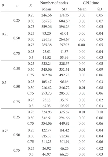
𝜃 𝜏 R Number of nodes CPU time

Mean SD Mean SD 0.25 0.25 0.25 246.56 174.35 0.00 0.05 0.50 367.78 604.59 0.00 0.07 0.75 359.06 396.26 0.00 0.05 0.50 0.25 93.20 61.04 0.00 0.04 0.50 226.18 264.67 0.00 0.05 0.75 285.38 297.02 0.00 0.05 0.75 0.25 25.01 41.37 0.00 0.04 0.5 44.52 55.99 0.00 0.03 0.5 0.25 0.25 323.24 228.37 0.00 0.05 0.50 345.06 332.54 0.01 0.09 0.75 362.94 492.78 0.00 0.06 0.50 0.25 105.47 96.16 0.00 0.03 0.50 216.62 246.72 0.01 0.08 0.75 293.75 285.05 0.00 0.06 0.75 0.25 23.18 35.97 0.00 0.02 0.5 67.08 105.95 0.00 0.03 0.75 0.25 0.25 324.93 326.67 0.01 0.10 0.50 346.91 294.66 0.00 0.06 0.75 354.06 449.82 0.00 0.06 0.50 0.25 122.77 114.42 0.00 0.04 0.50 215.55 217.34 0.00 0.04 0.75 341.23 301.91 0.00 0.06 0.75 0.25 26.92 46.26 0.00 0.02 0.5 46.97 66.25 0.00 0.03

Table 4: ANOVA table for the number of nodes with 𝑛 = 12 and 𝑃 = 0.5. Source SS DF MS F 𝑃 value 𝜃 2 113054 56527 0.74 0.48 (𝜏, R) 7 38742472 5534639 72.26 0.00 Error 2390 1.83𝐸 + 08 76593 Total 2399 2.22𝐸 + 08

0.50), (0.5, 0.75), (0.75, 0.25), and (0.75, 0.50). The mean and the standard deviation of the number of nodes and the mean and the standard deviation of the CPU time (in seconds) were reported for the branch-and-bound algorithm. 100 replications were randomly generated for each case and

the results were presented inTable 1. A two-way analysis of

variance (ANOVA) on the number of nodes of the

branch-and-bound algorithm was constructed and given inTable 2.

The resulting𝐹 value of factor 𝑃 was 189.52 with a 𝑃 value

close to 0, which indicated that the values of𝑃 really affect

the performance of the branch-and-bound algorithm. In fact,

problems are easier to solve when the value of 𝑃 is larger.

The main reason is thatProperty 2is more powerful in this

case. In addition, the resulting𝐹 value of due date factor 𝜏

(6)

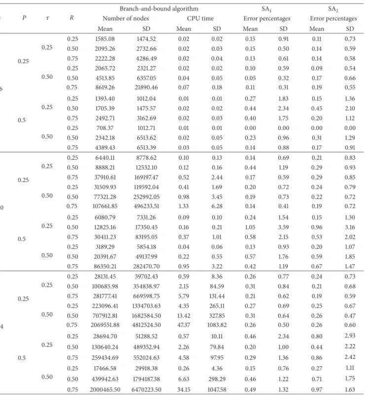
Table 5: The performance of the B&B and SA algorithms (𝜃 = 0.5).

n P 𝜏 R

Branch-and-bound algorithm SA₁ SA₂

Number of nodes CPU time Error percentages Error percentages

Mean SD Mean SD Mean SD Mean SD

16 0.25 0.25 0.25 1585.08 1474.52 0.02 0.02 0.15 0.91 0.11 0.73 0.50 2095.26 2732.66 0.02 0.03 0.15 0.50 0.14 0.59 0.75 2222.28 4286.49 0.02 0.04 0.13 0.61 0.14 0.58 0.50 0.25 2065.72 2321.27 0.02 0.02 0.10 0.59 0.09 0.54 0.50 4513.85 6357.05 0.04 0.05 0.05 0.32 0.17 0.66 0.75 8619.26 21890.46 0.07 0.18 0.11 0.31 0.19 0.55 0.5 0.25 0.25 1393.40 1012.04 0.01 0.01 0.27 1.83 0.15 1.36 0.50 1705.39 1475.57 0.02 0.02 0.44 2.34 0.45 2.10 0.75 2492.71 3162.69 0.02 0.03 0.40 1.75 0.20 1.12 0.50 0.25 708.37 1012.71 0.01 0.01 0.00 0.00 0.00 0.00 0.50 2342.18 6513.62 0.02 0.05 0.23 0.96 0.31 1.29 0.75 4389.43 6513.39 0.03 0.05 0.14 0.88 0.17 0.91 20 0.25 0.25 0.25 6440.11 8778.62 0.10 0.13 0.14 0.69 0.21 0.83 0.50 8888.21 12532.10 0.12 0.16 0.44 1.19 0.29 0.93 0.75 37910.61 169197.47 0.52 2.44 0.17 0.59 0.29 0.85 0.50 0.25 31509.93 119592.04 0.41 1.69 0.20 0.72 0.24 0.79 0.50 77321.28 252992.05 0.98 3.45 0.19 0.73 0.22 0.72 0.75 107661.85 496233.51 1.33 6.28 0.14 0.41 0.19 0.72 0.5 0.25 0.25 6080.79 7331.26 0.09 0.10 0.24 1.54 0.15 1.30 0.50 12825.16 17350.45 0.16 0.21 1.05 3.59 0.96 3.16 0.75 30411.23 83195.05 0.37 1.01 0.58 2.15 0.53 2.02 0.50 0.25 3189.29 5854.18 0.04 0.06 0.13 0.93 0.20 1.07 0.50 20391.67 49137.99 0.22 0.55 0.57 1.76 0.59 1.85 0.75 86350.21 282470.70 0.95 3.22 0.42 1.19 0.67 1.47 24 0.25 0.25 0.25 28131.45 39702.43 0.59 8.36 0.26 0.77 0.24 0.73 0.50 100685.98 354838.97 2.15 84.59 0.31 0.84 0.21 0.68 0.75 281777.41 669598.75 5.79 131.44 0.21 0.62 0.19 0.59 0.50 0.25 223096.41 1334703.63 4.35 265.11 0.27 0.69 0.25 0.67 0.50 707912.81 1682584.50 13.42 327.85 0.31 0.64 0.26 0.47 0.75 2069551.88 4812524.50 47.37 1083.82 0.26 0.50 0.26 0.60 0.5 0.25 0.25 28694.70 51288.52 0.57 10.11 0.46 2.34 0.80 2.93 0.50 130640.24 489352.94 2.26 79.84 0.20 1.00 0.44 2.22 0.75 259434.69 552024.63 4.58 97.95 0.29 1.36 0.86 2.42 0.50 0.25 17466.58 29918.38 0.26 4.36 0.15 0.76 0.27 1.11 0.50 439942.63 1794187.38 6.63 298.29 0.46 1.22 0.71 1.75 0.75 2000465.50 6470223.50 34.15 1047.58 0.49 1.32 0.97 1.63

the values of𝜏 or 𝑅 have statistically significant effects on the

difficulty of the problem. A closer look atTable 1revealed that

problems are easier to solve as𝑅 decreases or when 𝜏 = 0.75.

The main reason is thatProperty 2and the lower bound are

more powerful in those cases.

Similar to the first part of the experiment, the second part

was to test the effects of the coefficient𝜃 as well as the effects

of the due date factors𝜏 and 𝑅. The job size was fixed at 12,

and𝑃 was 0.5. Three different values of 𝜃 (0.25, 0.5, and 0.75)

and eight values of(𝜏, 𝑅) values were tested, that is, (0.25,

0.25), (0.25, 0.50), (0.25, 0.75), (0.5, 0.25), (0.5, 0.50), (0.5, 0.75), (0.75, 0.25), and (0.75, 0.50). As a consequence, 24 cases were tested and 100 replications were randomly generated

for each case. The results were presented inTable 3. A

two-way ANOVA on the number of nodes was utilized to test the effects of the parameters to the performance of the

branch-and-bound algorithm, and the result was reported inTable 4.

(7)

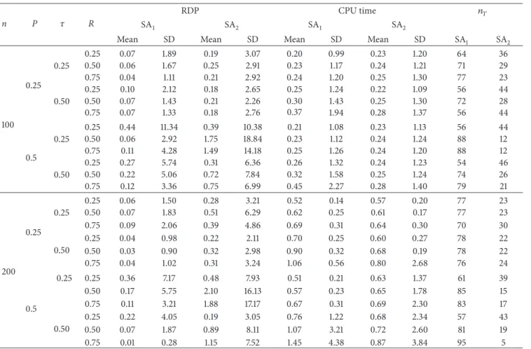
Table 6: The performance of the SA₁and SA₂algorithms with𝜃 = 0.5.

n P 𝜏 R

RDP CPU time 𝑛_𝑇

SA₁ SA₂ SA₁ SA₂

Mean SD Mean SD Mean SD Mean SD SA₁ SA₂

100 0.25 0.25 0.25 0.07 1.89 0.19 3.07 0.20 0.99 0.23 1.20 64 36 0.50 0.06 1.67 0.25 2.91 0.23 1.17 0.24 1.21 71 29 0.75 0.04 1.11 0.21 2.92 0.24 1.20 0.25 1.30 77 23 0.50 0.25 0.10 2.12 0.18 2.65 0.25 1.24 0.22 1.09 56 44 0.50 0.07 1.43 0.21 2.26 0.30 1.43 0.25 1.30 72 28 0.75 0.07 1.33 0.18 2.76 0.37 1.94 0.28 1.37 56 44 0.5 0.25 0.25 0.44 11.34 0.39 10.38 0.21 1.08 0.23 1.13 56 44 0.50 0.06 2.92 1.75 18.84 0.23 1.12 0.24 1.24 88 12 0.75 0.11 4.28 1.49 14.18 0.25 1.26 0.24 1.20 88 12 0.50 0.25 0.27 5.74 0.31 6.36 0.26 1.32 0.24 1.23 54 46 0.50 0.22 5.06 0.72 7.84 0.32 1.58 0.25 1.24 74 26 0.75 0.12 3.36 0.75 6.99 0.45 2.27 0.28 1.40 79 21 200 0.25 0.25 0.25 0.06 1.50 0.28 3.21 0.52 0.14 0.57 0.20 77 23 0.50 0.07 1.83 0.51 6.29 0.62 0.25 0.61 0.17 77 23 0.75 0.09 2.06 0.39 4.86 0.69 0.31 0.64 0.30 70 30 0.50 0.25 0.04 0.98 0.22 2.11 0.70 0.25 0.60 0.27 78 22 0.50 0.03 0.90 0.32 2.98 0.90 0.32 0.68 0.19 78 22 0.75 0.04 1.02 0.31 3.24 1.06 0.56 0.80 2.68 76 24 0.5 0.25 0.25 0.36 7.17 0.48 7.93 0.51 0.21 0.63 1.37 61 39 0.50 0.17 5.75 2.10 16.13 0.57 0.23 0.65 1.78 85 15 0.75 0.11 3.21 1.88 17.17 0.67 0.31 0.69 2.30 83 17 0.50 0.25 0.22 4.05 0.19 3.05 0.76 1.22 0.68 2.34 57 43 0.50 0.07 1.87 0.89 8.11 1.07 3.21 0.72 2.60 81 19 0.75 0.01 0.28 1.15 7.52 1.45 4.38 0.87 3.84 95 5

value of 0.48, which implied that𝜃 does not affect the

per-formance of the branch-and-bound algorithm. On the other hand, the statistical test showed that the due date factors have significant effects on the performance of the branch-and-bound algorithm, and the problems are easier to solve when 𝜏 = 0.75, which is consistent with the findings in the first part of the experiment.

The main purpose of the third part of the experiment was to study the impact of the number of jobs to the performance of the branch-and-bound algorithms and the accuracy of the proposed simulated annealing algorithms. Three different job sizes (𝑛 = 16, 20, and 24) were tested. Since the problems are

relatively easier to solve when𝜏 = 0.75 and 𝜃 was found to be

the insignificant factors in the second part of the experiments,

we ignored the cases when𝜏 = 0.75 and fixed 𝜃 at 0.5 in the

third part of the experiment. Two values of𝜏 (0.25, 0.50) and

three values of𝑃 (0.25, 0.50, and 0.75) and of 𝑅 (0.25, 0.50,

and 0.75) were tested. The mean and standard deviation of the number of nodes and the mean and standard deviation of the CPU time (in seconds) for the branch-and-bound algorithm were given, while only the mean and standard deviation of the error percentages of the SA algorithms were reported. The error percentage of the solution produced by SA is calculated as

(𝑉 − 𝑉∗₎

𝑉∗ × 100%, (12)

where𝑉 is the weighted combination of the total completion

time and the total tardiness of the solution generated by SA

and 𝑉∗ is the value of the optimal solution obtained from

the branch-and-bound algorithm. The execution time of SA algorithms was not recorded since they were finished within a second. For each condition, 100 replications were generated

and the results were given inTable 5. It is observed that the

branch-and-bound algorithm could solve problems of up to 24 jobs in a reasonable amount of time. However, the number of nodes and execution time grow exponentially as the number of jobs increases since the problem is NP-hard. The

most time consuming case(𝑛, 𝑃, 𝜏, 𝑅) = (24, 0.25, 0.5, 0.75)

took an average execution time of 47.37 seconds. As to the performance of the SA algorithms, the results showed that both of them are quite accurate with a mean percentage error of less than 1% for all the tested cases. Moreover, it seemed

that SA₂performed better than SA₁when the number of jobs

is 16; however, the trend is not obvious as the number of jobs becomes larger. Thus, we would study the performance of the algorithms for large job-size problems in the last part of the experiments.

We tested two job sizes, that is, 𝑛 = 100 and 200, in

the last part of the experiments. We randomly generated 100 instances for each situation and we reported the results inTable 6. The mean and standard deviation of the relative deviation percentage (RDP) were given. The RDP of the

(8)

solution produced by a simulated annealing algorithm is calculated as

(𝑉_𝑖− min {𝑉₁, 𝑉₂})

min{𝑉₁, 𝑉₂} × 100% (13)

for𝑖 = 1, 2, where 𝑉_𝑖is the value of the weighted combination

of the total completion time and the total tardiness of the jobs

from the first agent generated by the𝑖th simulated annealing

algorithm. The mean and standard deviation of the execution time were also reported. In addition, we recorded the number

of times (𝑛_𝑇) it yields the minimum value. It was seen that

both algorithms are very fast since the mean execution time is less than 1 second for all the tested cases. However, the first SA algorithm performs better than the second one in terms of the RDP values and the number of times it yields the minimum value. Thus, it is recommended as the number of jobs increases.

6. Conclusion

In this paper, we considered a two-agent single-machine scheduling problem where the objective is to minimize the weighted combination of the total completion time and the total tardiness of the jobs of the first agent given that no tardy job is allowed for the second agent. We proposed a branch-and-bound algorithm to solve the problem optimally and two simulated annealing algorithms to find near-optimal solutions. The computational experiments showed that the branch-and-bound algorithm could solve problems of up to 24 jobs in a reasonable amount of time. It also showed that the performance of the first SA algorithm is very good, yielding an average error percentage of less than 1% for all the tested cases.

Conflict of Interests

The authors declare that there is no conflict of interests regarding the publication of this paper.

Acknowledgments

The authors are grateful to the referees for their comments. This work is supported by the National Science Council of Taiwan, under Grant no. NSC 1000-2221-E-035-029-MY3.

References

[1] M. Pinedo, Scheduling: Theory, Algorithms and Systems, Springer, New York, NY, USA, 3rd edition, 2008.

[2] R. Rudek, “Computational complexity and solution algorithms for flowshop scheduling problems with the learning effect,” Computers and Industrial Engineering, vol. 61, no. 1, pp. 20–31, 2011.

[3] J. B. Wang and J. J. Wang, “Single machine scheduling with sum-of-logarithm-processing-time based and position based learn-ing effects,” Optimization Letters, 2012.

[4] S. J. Yang, “Unrelated parallel-machine scheduling with deterio-ration effects and deteriorating multi-maintenance activities for

minimizing the total completion time,” Applied Mathematical Modelling, vol. 37, pp. 2995–3005, 2012.

[5] J. M. Peha, “Heterogeneous-criteria scheduling: minimizing weighted number of tardy jobs and weighted completion time,” Computers and Operations Research, vol. 22, no. 10, pp. 1089– 1100, 1995.

[6] P. J. Brewer and C. R. Plott, “A binary conflict ascending price (BICAP) mechanism for the decentralized allocation of the right to use railroad tracks,” International Journal of Industrial Organization, vol. 14, no. 6, pp. 857–886, 1996.

[7] M. A. Kubzin and V. A. Strusevich, “Planning machine mainte-nance in two-machine shop scheduling,” Operations Research, vol. 54, no. 4, pp. 789–800, 2006.

[8] K. R. Baker and J. C. Smith, “A multiple-criterion model for machine scheduling,” Journal of Scheduling, vol. 6, no. 1, pp. 7– 16, 2003.

[9] A. Agnetis, P. B. Mirchandani, D. Pacciarelli, and A. Pacifici, “Scheduling problems with two competing agents,” Operations Research, vol. 52, no. 2, pp. 229–242, 2004.

[10] T. C. E. Cheng, C. T. Ng, and J. J. Yuan, “Multi-agent scheduling on a single machine to minimize total weighted number of tardy jobs,” Theoretical Computer Science, vol. 362, no. 1–3, pp. 273– 281, 2006.

[11] C. T. Ng, T. C. E. Cheng, and J. J. Yuan, “A note on the complexity of the problem of two-agent scheduling on a single machine,” Journal of Combinatorial Optimization, vol. 12, no. 4, pp. 387– 394, 2006.

[12] K. B. Lee, B.-C. Choi, J. Y.-T. Leung, and M. L. Pinedo, “Approxi-mation algorithms for multi-agent scheduling to minimize total weighted completion time,” Information Processing Letters, vol. 109, no. 16, pp. 913–917, 2009.

[13] A. Agnetis, G. Pascale, and D. Pacciarelli, “A lagrangian ap-proach to single-machine scheduling problems with two com-peting agents,” Journal of Scheduling, vol. 12, no. 4, pp. 401–415, 2009.

[14] W.-C. Lee, W.-J. Wang, Y.-R. Shiau, and C.-C. Wu, “A single-machine scheduling problem with two-agent and deteriorating jobs,” Applied Mathematical Modelling, vol. 34, no. 10, pp. 3098– 3107, 2010.

[15] J. Y.-T. Leung, M. Pinedo, and G. H. Wan, “Competitive two-agent scheduling and its applications,” Operations Research, vol. 58, no. 2, pp. 458–469, 2010.

[16] Q. Q. Nong, T. C. E. Cheng, and C. T. Ng, “Two-agent sched-uling to minimize the total cost,” European Journal of Opera-tional Research, vol. 215, no. 1, pp. 39–44, 2011.

[17] P. Liu, N. Yi, and X. Zhou, “Two-agent single-machine schedul-ing problems under increasschedul-ing linear deterioration,” Applied Mathematical Modelling, vol. 35, no. 5, pp. 2290–2296, 2011. [18] T. C. E. Cheng, Y. H. Chung, S. C. Liao, and W. C. Lee,

“Two-agent singe-machine scheduling with release times to minimize the total weighted completion time,” Computers & Operations Research, vol. 40, pp. 353–361, 2013.

[19] X. Yu, Y. Zhang, D. Xu, and Y. Yin, “Single machine scheduling problem with two synergetic agents and piece-rate mainte-nance,” Applied Mathematical Modelling, vol. 37, no. 3, pp. 1390– 1399, 2013.

[20] P. Liu, N. Yi, X. Zhou, and H. Gong, “Scheduling two agents with sum-of-processing-times-based deterioration on a single machine,” Applied Mathematics and Computation, vol. 219, pp. 8848–8855, 2013.

(9)

[21] J. Du and J. Y. T. Leung, “Minimizing Total Tardiness on one Machine is NP-hard,” Mathematics of Operations Research, vol. 15, pp. 483–495, 1990.

[22] M. Soolaki, I. Mahdavi, N. Mahdavi-Amiri, R. Hassanzadeh, and A. Aghajani, “A new linear programming approach and genetic algorithm for solving airline boarding problem,” Applied Mathematical Modelling, vol. 36, no. 9, pp. 4060–4072, 2012. [23] R. Ramezanian and S. M. Mohammad, “Hybrid simulated

annealing and MIP-based heuristics for stochastic lot-sizing and scheduling problem in capacitated multi-stage production system,” Applied Mathematical Modelling, vol. 37, pp. 5134–5147, 2013.

[24] E. Atmaca and A. Ozturk, “Defining order picking policy: a storage assignment model and a simulated annealing solution in AS/RS systems,” Applied Mathematical Modelling, vol. 37, pp. 5069–5079, 2013.

[25] S. M. Goldansaz, F. Jolai, and A. H. Z. Anaraki, “A hybrid impe-rialist competitive algorithm for minimizing makespan in a multi-processor open shop,” Applied Mathematical Modelling, vol. 37, no. 23, pp. 9603–9616, 2013.

[26] S. Kirkpatrick, C. D. Gelatt Jr., and M. P. Vecchi, “Optimization by simulated annealing,” Science, vol. 220, no. 4598, pp. 671–680, 1983.

[27] D. Ben-Arieh and O. Maimon, “Annealing method for PCB assembly scheduling on two sequential machines,” International Journal of Computer Integrated Manufacturing, vol. 5, pp. 361– 367, 1992.

(10)

Submit your manuscripts at

http://www.hindawi.com

Hindawi Publishing Corporation

http://www.hindawi.com Volume 2014

Mathematics

Journal of

Hindawi Publishing Corporation http://www.hindawi.com

Differential Equations

International Journal of

Volume 2014

Applied MathematicsJournal of

http://www.hindawi.com Volume 2014 Mathematical PhysicsAdvances in

Complex Analysis

Journal of

Optimization

Journal of

Combinatorics

International Journal of

Journal of Hindawi Publishing Corporation

Function Spaces

Abstract and Applied Analysis

http://www.hindawi.com Volume 2014 International Journal of Mathematics and Mathematical Sciences

Hindawi Publishing Corporation http://www.hindawi.com Volume 2014

The Scientific

World Journal

Discrete Dynamics in Nature and Society Hindawi Publishing Corporation

http://www.hindawi.com Volume 2014 Hindawi Publishing Corporation

Discrete Mathematics

Journal of

Single-Machine Scheduling to Minimize Total Completion Time and Tardiness with Two Competing Agents

Research Article