Abstract—In recent years, smart devices have become
ubiquitous. Many of these devices are equipped with global positioning system (GPS), Wi-Fi, and other sensors. With their high mobility, the idea of “mobile devices as probes” has been attracting more and more attention. Mobility and flexibility offered by smart mobile devices are what traditional fixed sensors lack. However, mobile devices’ power supplies are quite limited. Although GPS is accurate, its high power consumption somewhat limits its accessibility and sustainability. In contrast, Wi-Fi is less power-hungry, but at the same time, less accurate. For the sake of sustainability, by adopting Wi-Fi as an alternative to GPS, longer operation is attainable at the cost of losing some degree of accuracy. In this paper, a Wi-Fi-based algorithm based on log-normal probability distribution of distances with respect to received signal strength is proposed. It is suitable for an outdoor environment where Wi-Fi Access Points (APs) are abundant. Simulations are conducted over known AP locations, and results show that the proposed algorithm can save, on average, as much as 35% more battery power than GPS does; the average localization error is about 18 meters, and the average velocity estimation error is about 25%.
Index Terms—Mobile phone sensing, Wi-Fi-based localization,
received signal strength indicator, log-normal distribution, positioning algorithm
I. INTRODUCTION
N recent years, smart mobile devices have become so prevalent. With the advent of new technologies, their sizes are now smaller and prices also cheaper. Most of them are equipped with many kinds of hardware sensors, such as accelerometer, global positioning system (GPS), magnetic field sensor, et cetera. Different wireless networking standards are supported too, for example, general packet radio service (GPRS), Wi-Fi, and Bluetooth [1, 2]. People carry their devices wherever they go, and help them with lots of their daily routines. As a matter of fact, those devices now play a very important role in our daily life. The number of smart mobile devices in active use today is on the rise.
Traffic information is of great importance to commuters and drivers. Traditionally, traffic condition monitoring relies on
Chi-Hua Chen is with the Telecommunication Laboratories, Chunghwa Telecom Co., Ltd., Taoyuan, Taiwan. (e-mail: [email protected]).
Chi-Ao Lee is with the Department of Information Management and Finance, National Chiao Tung University, Hsinchu, Taiwan. (e-mail: [email protected]).
Chi-Chun Lo is with the Department of Information Management and Finance, National Chiao Tung University, Hsinchu, Taiwan. (e-mail: [email protected]).
stationary roadside sensors which are deployed at some predetermined locations. Once deployed, their locations are seldom changed. If more road sections are to be monitored, more sensors have to be deployed at those locations, which is laborious and costly.
Nowadays, smart devices seem to be ubiquitous. Their capabilities offer new opportunities for data collection. The idea of “mobile devices as probes” has begun to gain much more attention than ever, since the necessary infrastructure, such as base stations, wireless access point (AP), and so forth, are already in place [3]. End users can write their own programs and install them on their devices. Information can then be retrieved from devices to perform real-time profiling and data collection of the surrounding environment. Large areas can be covered while mobile devices are on the move. They form a very large wireless sensor network (WSN). Mobility and flexibility offered by smart mobile devices are what traditional stationary sensors lack [4].
Power supply is a major concern for most mobile devices. Due to their relatively small size and light weight, their power supply relies heavily on the battery they carry. Some of the on-device sensors consume more battery power than others. If used continuously for a prolonged period of time, battery would be drained out in no time. GPS is one of those power-hungry sensors. Although localization accuracy of GPS is fine, the characteristic of high power consumption somewhat limits its availability and sustainability. Besides, some devices do not come with GPS [5] since it is considered unnecessary. Moreover, GPS does not work when inside a building. To make it worse, in urban cities where the skyline is made up of lots of tall skyscrapers which, to some extent, block the view of the sky, also known as “urban canyons [6]”, GPS works poorly.
Wi-Fi, on the other hand, consumes less power compared with GPS. It even works in indoor environments where there are Wi-Fi APs around. If coverage area of APs is large, localization accuracy can be improved. Years before, Taipei City Government had begun to widely deploy Wi-Fi APs all over Taipei City [7]. As the number of APs is increasing, these APs can be exploited for the purpose of localizing an object. In this paper, a Wi-Fi-based algorithm for vehicle localization and velocity estimation is proposed. Some accuracy of localization and velocity estimation is lost in exchange for keeping mobile devices functional longer to collect as much traffic information as possible.
This paper is organized as follows. Section II discusses the related work in detail. The proposed algorithm is discussed in
Vehicle Localization and Velocity Estimation
Based on Mobile Phone Sensing
Chi-Hua Chen, Chi-Ao Lee, Chi-Chun Lo
Section III. Section IV presents the experiment results. Finally, conclusions and future work are given in Section V.
II. RELATED WORK
In this section, range-based localization algorithms and range-free localization algorithms are discussed in following subsections.
A. Range-based Localization Algorithms
Range-based localization algorithms require precise measurement of distance, angle, or propagation time. Commonly-seen methods include: time of arrival (TOA), time difference of arrival (TDOA), and received signal strength indicator (RSSI) –based.
1) Time of Arrival
Time of arrival (TOA) measures the travel time of a radio signal from a transmitter to a remote receiver. Transmitter-receiver separation (radius) can be measured by the time the signal is sent from the transmitter and the time it is received by the receiver, plus the traveling speed of signal. The target lies on the circle centered at the transmitter with radius estimated above. Data from three or more transmitters/receivers are needed to narrow down the target location. The algorithm to localize the target of interest uses geometry to calculate the intersection of circles [8], which is called “trilateration [9]” and discussed as follows.
Suppose there are three nodes, A, B, and C, located at (xA, yA),
(xB, yB), and (xC, yC) respectively. The distance between and the
target node and each of A, B, and C has been determined to be rA, rB, and rC respectively. The trilateration process is to find a
point (x', y') that minimizes ω by solving Equation (1) [9].
C C C B B B A A A
r
y
y
x
x
r
y
y
x
x
r
y
y
x
x
2 2 2 2 2 2)
'
(
)
'
(
)
'
(
)
'
(
)
'
(
)
'
(
(1)By observing Equation (1), one can find out that in order to minimize ω, each term in (1) must be zero. Node A, B, and C can be thought of as APs, radius rA, rB, and rC the
transmitter-receiver separation, and the three circles the coverage areas of the three APs. If ω equals zero, this implies that the three coverage areas intersect at one point P, shown in Figure 1(a).
Fig. 1. (a) Three circles intersect at one point P [8], (b) Three circles overlap each other [10].
However, in reality, this is not always the case. Instead, coverage areas overlap each other most of the time, as shown in Figure 1(b), since transmitter-receiver separation measurement has some inherent errors. The point of interest that minimizes ω then lies in the overlapping area.
GPS, for example, is one of those systems that adopt TOA algorithm [11]. TOA requires precise synchronization between transmitters and receivers. Dedicated hardware, which has high power consumption, is required to perform this task.
2) Time Difference of Arrival
Time difference of arrival (TDOA) uses the arrival time difference (TD) of a signal at some spatially separated receivers to determine the target’s location. It can operate in two modes which are illustrated in following subsections.
a) Mode 1
In Loran-C [12] -like systems, wavelets are sent from three or more transmitters (reference nodes). One of those transmitters serves as master, and the rest of them as secondaries [13]. The receiver (the target of interest, TOI) measures the subtle differences in the time it takes for wavelets to be received by the receiver. The localization procedure is on the receiver.
b) Mode 2
In contrast, in this mode, the target of interest emits a reference wavelet to multiple fixed reference nodes. These fixed nodes then forward TD information to a centralized controller to run the localization procedure.
Each pair of two fixed nodes can determine a hyperbola to which all possible locations of the target that has a constant differential distance can be mapped. Location estimation is the intersection of all hyperbolas. Like TOA, special hardware and power consumption are major drawbacks. [14] is one of those systems that adopt TDOA.
3) RSSI-based
For some localization algorithm, distance measurement is required. To obtain an estimated transmitter-receiver separation, log-distance path loss model [15] is used in [16]. As electromagnetic wave propagates through space, its power density reduces routes. According to this model, the received signal strength (RSS) in dB at distance d is given by (2), where npathloss indicates rate of path loss increase with distance, and D0 is a reference distance from the transmitter. D0 and 𝑃𝐿𝐷0 are often determined empirically. npathloss varies depending on
surrounding environments. It is determined empirically. Table I shows typical values of npathloss in different situations [17, 18].
0log
10
0D
d
n
PL
PL
d D pathloss (2)In fact, even when the distance between transmitter and receiver is the same, the RSS might differ. This is the result of terrain variation and obstacles in between, also known as “shadowing effect [19]”, which is a factor [16] failed to consider. Using (2), if RSS is the same, the inferred distance
between transmitter and receiver will always be the same. In real-life situations, this is not always the case. Experiments conducted by John J. Egli [20] showed and it is now widely accepted that RSS fluctuates with a log-normal distribution (lnƝ(μ,σ)) with respect to distance. Taking shadowing effect into account, Equation (2) becomes (3), where Xσis a Gaussian
random variable with zero mean and standard deviation σ, and is determined empirically.
X
D
d
n
PL
PL
d D pathloss
0log
10
0 (3) TABLEIVALUES OF PATH LOSS EXPONENT IN DIFFERENT ENVIRONMENTS [17]
Environment VALUE OF NPATHLOSS
Free space 2
Urban area cellular radio 2.75 ~ 3.5
Urban area cellular radio with shadowing effect 3 ~ 5
Indoor line-of-sight 1.6 ~ 1.8
Indoor line-of-sight with obstacles 4 ~ 6
Upon receiving signal from a transmitter, RSS can be computed. Plug known parameters into (3) and solve the equation, distance can be determined for used in other localization algorithms.
B. Range-free Localization Algorithms
This type of localization algorithms are relatively simple compared with range-based ones.
1) Centroid Localization
Arvind Thiagarajan et al. [5] proposed a traffic delay estimation algorithm, in which two algorithms are used to determine user’s current location. One algorithm acquires GPS coordinates every second to form user’s traveling trace. Velocity can then be easily calculated by dividing the distance between two sampling points by the time difference between these two points. Nevertheless, as mentioned above in Section I, higher GPS coordinates acquisition rate often leads to shorter lifetime. The other algorithm adopts a range-free scheme. Wi-Fi scan is performed continuously with a predefined time interval between each scan. Locations of nearby APs observed during the scan are looked up in a war driving [21] database established in advance. User’s location is approximated by the centroid localization (CL) algorithm [22].
In CL settings, there are multiple anchor nodes with known locations and overlapping coverage. All anchor nodes are synchronized so that their beacon signals do not overlap in time. The target listens for a fixed time period t, and calculates the connectivity metric (CMi), defined in (4), for every anchor node
it discovers. The target infers its location (x', y') by selecting a set of anchor nodes from those discovered whose CMs exceed a certain threshold and calculating the center of gravity (Equation (5)) of this set of nodes.
100
, ,
i sent i received iN
N
CM
(4)
AP AP n i i AP n i i APy
n
x
n
y
x
1 11
,
1
)
'
,
'
(
(5)The CL algorithm has one weakness: It is easily affected by one or more APs that are located relatively farther away from the rest of the APs, the so-called “outliers” in statistical terms. For instance, in Figure 2, if access point H is not taken into account, the approximated location is, say, at point P; if H is taken into account, the localization result would be drawn toward H to P' [23]. The higher localization error of outlier is generated by using this algorithm.
Fig. 2. Impact of outliers on localization result [23].
2) Weighted-Centroid Localization
Jan Blumenthal et al. [24] proposed a weighted-centroid localization (WCL) algorithm which attempt to reduce the effect of outliers. Equation (5) can be expressed as Equation (6), where every AP has the same weight, 1. But in WCL algorithm, each AP is assigned with a different weight. Equation (6) can then be re-written as a more general form, as in (7).
AP AP AP AP n i i n j n i i n jy
x
y
x
1 1 1 11
1
1
,
1
1
1
)
'
,
'
(
(6)
AP AP AP AP n i i i n j j n i i i n j jy
w
w
x
w
w
y
x
1 1 1 11
,
1
)
'
,
'
(
(7)In [24], the weight is defined by (8). APs that are closer to the target are weighted more than those that are farther away from the target. Therefore, weight and distance are inversely related. In order to further reduce the effect of outlier APs, the distance is raised to a power g. g i i
d
w
1
(8)This WCL requires distance estimation. Frii’s free space propagation model [25] is used (Equation (9)). In real-life environments, this model is not practical, as radio signal is interfered [24] by obstacles between transmitter and receiver, multipath, shadowing effect, diffraction at edges, absorption of electromagnetic radiation, reflection, etc.
2
4
TR R T T Rd
G
G
P
P
(9) 3) APITAPIT [26] is an area-based localization algorithm. It performs a point-in-triangulation (PIT) test to narrow down possible area in which the target lies. PIT test is conducted as follows. First, arbitrarily select three nodes from candidate anchor nodes (nodes discovered by scanning) and check if the target is inside the triangle formed by these three nodes. After exhausting all
3
APn
triplets of nodes, APIT estimates the target’s location
to be the center of gravity of the intersection of all triangles. A perfect PIT test is not feasible in real situation, therefore approximate PIT (APIT) test is used instead. In APIT test, if a node P is inside △ ABC, when none of P’s neighboring nodes are closer to/further from (the departure test) all three vertices at the same time, P is inside the triangle; otherwise P is outside the triangle. The assumption that the longer the distance the weaker the RSSI is also made in inside/outside decision making of departure test. In order to improve inside-outside accuracy, more neighboring nodes must be taken into account. Therefore, APIT has higher demand on the number of nodes required to perform localization. Also the computation overhead is high as the number of neighboring nodes grows.
III. AWI-FI-BASED ALGORITHM FOR VEHICLE LOCALIZATION AND VELOCITY ESTIMATION
A localization algorithm which makes use of the public Wi-Fi infrastructure is proposed in order to overcome the drawbacks of traditional fixed traffic monitoring system. It is detailed in this section.
A. Problem Definition
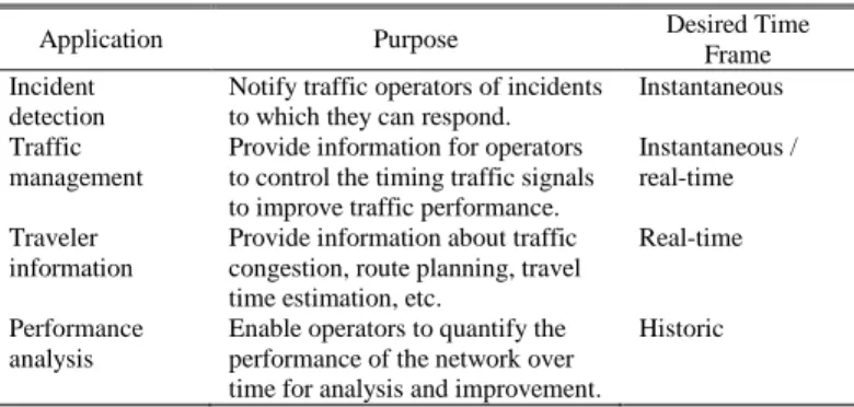
Real-time traffic information is of great value to commuters, driver, and traffic operators. Data collected can be used in many applications, just to name a few (Table II).
TABLEII
REAL-TIME TRAFFIC INFORMATION APPLICATIONS
Application Purpose Desired Time
Frame Incident
detection
Notify traffic operators of incidents to which they can respond.
Instantaneous Traffic
management
Provide information for operators to control the timing traffic signals to improve traffic performance.
Instantaneous / real-time Traveler
information
Provide information about traffic congestion, route planning, travel time estimation, etc.
Real-time
Performance analysis
Enable operators to quantify the performance of the network over time for analysis and improvement.
Historic
As mentioned earlier in Section II, the traditional stationary traffic monitoring system is not flexible enough. The emerging opportunities of “mobile devices as probes” seem like potential alternatives. Many researchers have been exploiting this idea
and propose many applications that make use of GPS or Wi-Fi. GPS has high accuracy. It requires dedicated electronics that have high power consumption, making it less suitable for mobile devices to operate for a prolonged period of time. Sampling GPS coordinates continuously with a very short time interval between each sampling drains out the battery in no time. On the contrary, Wi-Fi is less power-hungry. Its localization accuracy is not as good as that of GPS, but still within acceptable range. Like many other algorithms, Wi-Fi is used for localization in this paper. It can operate much longer than GPS does, but at the cost of accuracy. Devices that have sustained power supply are out of the scope of this paper.
B. The Proposed Localization Algorithm
The proposed localization algorithm is elaborated in detail in this section.
1) Model Building
Due to shadowing effect [19], RSSI varies even at the same location. According to [20], RSSI fluctuates with a log-normal distribution instead of a uniform distribution. If log-distance shadowing model (Equation (3)) is used to infer the transmitter-receiver separation, sometimes the inferred distance could be somewhat unreasonable (the probability, with RSSI fixed, is too small). If the inferred distances are used in WCL [24], the corresponding APs would be over weighted (when the inferred distance is very close) or underweighted (when the inferred distance is too far away). That is the reason why probability is taken into consideration in the proposed localization algorithm to augment weight determination.
Like [27], log-normal distribution models of different RSSIs must be built for every AP in the WSN. The probability density function (PDF) is defined in Equation (10) [28].
lnƝ(μ,σ)= 2 2 2 ) (ln 2
2
1
de
d
(10)To build the model for different RSSIs, there are two parameters that need to be determined, that is, mean μ and standard deviation σ. To begin with, APs’ locations must be identified. Then, at every distance, the receiver scans for nearby APs and records their RSSI values. The receiver also rotates about APs to record RSSI values in order to accommodate environmental variations. This process should be repeated for every AP in the network to build a complete profile (database) of the environment for later use in the localization procedure.
2) Localization Algorithm
The proposed localization algorithm has three steps.
a) Step 1
After scanning for nearby APs, suppose n APs are discovered. Their respective RSSIs r1, r2, …, rn are recorded. Each AP is assigned with a weight wi according to the weight function (11),
where di is the estimated distance between the i-th AP and the
target,
p
i,RSSI is the probability that the distance betweendi is estimated using (3). To calculate
p
i,RSSI , thecorresponding parameters μ and σ must be looked up in the database created in advance (Section III.B.1). If n = 2, WCL with weight function (11) is used instead as the final estimation result, and there is no need to go through Step 2 and 3.
g i RSSI i i
d
p
w
, (11) b) Step 2Arbitrarily select n-1 APs (AP1, AP2, …, APj-1, APj+1, …, APn , j = 1, 2, …, n) from those discovered in Step 1, and then “multilateration” [29] is applied on these n-1 APs. Trilateration is merely a special case of multilateration. Equation (1) can be rephrased as a more general form, as in (12). After multilateration, the resulting point (x'j , y'j) is assigned with a
weight w'j, as defined in (13).
n
j
d
y
y
x
x
d
y
y
x
x
d
y
y
x
x
d
y
y
x
x
d
y
y
x
x
d
y
y
x
x
n j i i i j i j n n j n j j j j j j j j j j j j j j j j...,
,
2
,
1
where
,
)
'
(
)
'
(
)
'
(
)
'
(
...
)
'
(
)
'
(
)
'
(
)
'
(
...
)
'
(
)
'
(
)
'
(
)
'
(
2 2 2 2 1 2 1 2 1 1 2 1 2 1 2 2 2 2 2 1 2 1 2 1
(12)n
j
w
w
w
w
w
w
w
n j i i n j j j...,
,
2
,
1
where
,
...
...
'
1 2 1 1
(13) c) Step 3According to [23], the closer the anchor points are to the target,
the better the approximation. After exhausting all
1
n
n
n-1–tuples, there will be n points which are closer to the target than those APs discovered in Step 1. The target’s real location can be narrowed down to a smaller region. Then WCL with weight function (13) is applied on these n points to arrive at the final estimation result.
3) Discussion
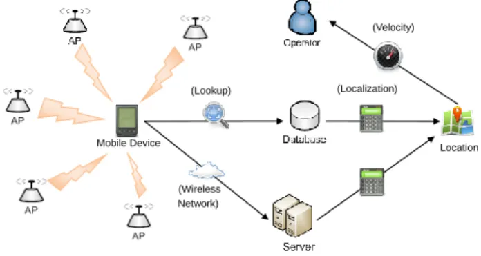
Range-based localization algorithms require dedicated hardware that usually have high power consumption; range-free algorithms are simple, but they can only narrow down possible location of TOI to a smaller region. The proposed algorithm adopts a fingerprint-like hybrid method (Figure 3). Probabilities are included to reduce the unfavorable effect of outliers. Thus, the proposed algorithm can achieve better approximation of TOI, and does not consume as much battery power as GPS does.
Mobile Device (Wireless Network) (Lookup) (Localization) Location (Velocity)
Fig. 3. Architecture & data flow.
However, the proposed algorithm has some inherent constraints. It requires that APs be abundant and their locations be known, and log-normal models be built in advance; radio transmission may be interfered more severely in indoor environment than in outdoor environment, so the proposed algorithm is more suitable for outdoor environment. Although its localization accuracy is not as good as that of GPS, it is still acceptable in outdoor environment and velocity estimation since vehicles are on the move and their velocity keeps changing too.
IV. SIMULATIONS &RESULT ANALYSES
In order to evaluate the accuracy of localization and velocity estimation, a simulation environment is built. This section gives out the detail of the simulation environment and analysis of the results.
A. Simulation Settings
Simulation settings, parameters, localization algorithms to be compared with, platforms, and programming languages used in this paper are described as follows. Performance metrics are also defined in this section.
1) Basic Assumptions
The proposed algorithm requires that APs’ locations be known and log-normal models be built in advance and both of them be stored in database. This database is stored on the device. If this algorithm is deployed on a metropolitan scale, the size of the database could be very large, making it not suitable for being stored on mobile devices due to their limited resources and capabilities. In this situation, the database and localization procedure might be offloaded to a centralized server. Nevertheless, this would require that mobile devices be
connected to a network to communicate with the server. More processing overheads as a result of communications with the server are needed, and thus consume more battery power. This is out of the scope of this paper.
In addition, each AP’s radio transmission pattern, once determined and stored in database, is assumed to be constant across time and fluctuates with a log-normal distribution.
2) Simulation Design
In order to simulate radio transmission of APs, experiments (Section III.B.1) are conducted on Nation Chiao Tung University campus to collect data. A tablet PC is used to record, at every distance, RSSI values of APs whose locations have been identified. The tablet is also rotated about APs to accommodate environmental variations. The parameters, i.e. mean and standard deviation, of log-normal probability models, plus the Gaussian random variable Xσ and the path loss
exponent npathloss in Equation (3), are determined based on the
collected data.
Theoretically speaking, Xσ has a zero mean. The path loss
exponent that makes the mean of the distribution closest to zero is chosen as npathloss (Figure 4). In the experiment, these two parameters are determined to be npathloss = 3.219 and Xσ ~
Ɲ(-0.00387252905148583, 7.998845433145), and are used in later simulation. Figure 5 shows the frequency and the PDF of the corresponding normal distribution.
Fig. 4. PDFs of different path loss exponents.
Fig. 5. Frequency of △RSSI2 and PDF.
The t-test [30] with H0 (null hypothesis): μ= 0 and H1 (alternative hypothesis): μ ≠ 0 is also performed. With confidence level α=5%, the t-statistics t = -0.082770267 does not lie in the rejection region | t | > tα=5%, n→∞, so H0 is not
rejected.
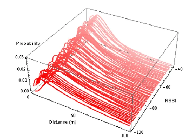
With the same set of data, log-normal models of different RSSIs with respect to distances can be built, as shown in Figure 6.
Fig. 6. PDFs of distances for different RSSIs.
After determining those parameters, RSSI can be generated by using a method often appears in genetic algorithms called “fitness proportionate selection [31]”. The method is described as follows. At first, a random sample location is generated. The distance di’s between this sample location and each AP are
calculated using surface distance [32]. Then, at distance di, a
vertical plane is drawn to get a cross-section of probabilities (
i
RSSI i
p
, ) of this distance at different RSSI levels (Figure 7). Next, these probabilities are normalized and then sorted in ascending order. A random number r is generated. Finally, the interval in which this random number r falls is found (as illustrated in Figure 8, interval I4) by calculating the cumulative probabilities, and the RSSI value corresponding to this interval is chosen as the received RSSI value from this AP.Fig. 7. Cross-section of probabilities.
Fig. 8. Fitness proportionate selection example [33]. …. ……
0 1
I1 I2 I3 I4 I5 In-1 In
The g values in the weight function (8) and (11) must ensure that APs which are far away are still effective [24]. A large g would make APs with relatively longer distances ineffective in location approximation. Estimation result would be drawn to the closest AP. A small g would, on the other hand, make every AP has similar weight. Outlier APs thus have greater impact on the localization result. To determine the optimal g value in (8) and (11), different values of g are tested in the simulated WSN. Optimal values are selected for four different scenarios (random/uniform distribution & homogeneous/heterogeneous APs).
As shown in Appendix A, in uniform distribution environment, the difference between weights of every AP should be relatively small, which can be achieved by a smaller g value. For example, suppose the weights of two APs are 0.1 and 0.0001 respectively. Let’s say if g = 1, the first AP weights a thousand times more than the second. Now if g = 1 10⁄ , their weights become
0
.
1
100
.
794
1
and0
.
0001
100
.
398
1
respectively. The first AP now weights only about 2 times more than the second. In random distribution settings, outliers should be weighted less. The value of g should not be too large (decrease the impact of relatively far away APs) or too small (increase the impact of outliers). Values of g used in the simulation are summarized in Table III.
TABLEIII
SUMMARY OF OPTIMAL g VALUES
AP AP type
Distribution Homogeneous Heterogeneous
Uniform WCL: 1 4.5⁄ WCL: 1 8⁄ The proposed: 1 4.5⁄ The proposed: 1 8⁄ Random WCL: 1 2⁄ WCL: 1 3.5⁄
The proposed: 1 2⁄ The proposed: 1 3.5⁄
To measure the lifetime of a specific localization algorithm, a program is developed and installed on the device. For GPS, coordinate information is acquired every second. For Wi-Fi-based localization algorithms, a Wi-Fi scan is performed every second, followed by the localization process. The battery is fully charged before each test. Since the device screen goes off after idling for a while, it is kept on for convenience of observation. No need to press the Power button to check whether the device is down due to low battery level or just idling.
3) Platforms & Programming Languages
The simulation environment is built on a computer with Windows 7 Professional SP1 64-bit operating system, Intel® Core™ i3 2.93 GHz CPU, 4 GB of memory. Localization simulation and velocity estimation programs are written in Java language.
A Samsung Galaxy Tab, 4000 mAh battery, 512 MB of memory, Samsung Exyons 3110 ARM Cortex A8 1.0 GHz CPU, upgraded to Android 2.3.3 system, is used for data collection to build models (Section III.B.1). It is equipped with
GPS, Wi-Fi 802.11 b/g/n, Bluetooth 3.0, GSM/GPRS/EDGE, et cetera. All data recorded are stored in SQLite databases on the device. Battery power consumption tests are also conducted on this device. Android systems support Java language, as well as C language. With a view to improve performance (the time required to give out a localization result), the computation-intense localization procedures are written in C language. Other Wi-Fi-related code uses Android’s standard APIs.
4) Case Design
The proposed localization algorithm is compared with the following algorithms mentioned in previous sections.
i. CL (Section II.B.1)
ii. WCL (Section II.B.2) with distances determined using (3)
iii. Trilateration (Section II.A.1) with distances determined using (3)
iv. APIT (Section II.B.3)
The localization simulation is built on a 100 by 100 m2 area. Two scenarios are studied: i) All APs are assumed to be homogeneous. That is, they all have the same log-normal models with respect to distances. ii) APs are heterogeneous. Their log-normal models differ in mean and variance.
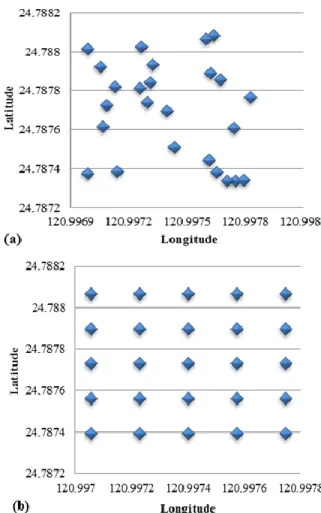
Besides, APs are scattered in two ways (Figure 9):
i. Random: APs are scattered at random in the simulation area, as in [23].
ii. Uniform: The simulation area is divided into 25 cells
(5 by 5). APs are placed at the center of each cell. Therefore, there are a total of four cases, i.e. uniform distribution + homogeneous APs (uni_homo), uniform distribution + heterogeneous APs (uni_hetero), random distribution + homogeneous APs (rand_homo), and random distribution + heterogeneous APs (rand_hetero). In velocity estimation, these four cases are studied, too.
On the grounds that real traffic condition is too complicated to be expressed as a mathematical model, traffic simulation software is used to generate sample locations of vehicles. VISSIM [34] is one of the best known microscopic multi-modal traffic flow simulation software in the world, and it is the simulation software used in this paper.
As for locations of APs, with a view to be more realistic, known AP locations are used in the random distribution cases. They are obtained from a provider, Qon [35]. The selected road section is shown in Appendix B, on which a simulated traffic flow is built. Some of the traffic simulation parameters are listed in Table IV. AP distributions are shown in Figure 10.
TABLEIV
SOME PARAMETERS OF THE TRAFFIC SIMULATION
Parameter Value
Period 3600 Simulation second Random Seed 1114
Simulation Resolution 1 time step(s)/Sim.sec. Driving Behavior Urban (motorized) Signals
Fig. 10. AP distribution in velocity estimation.
5) Performance Metrics
To evaluate how well each localization algorithm performs, some performance metrics are defined below.
a) Localization accuracy
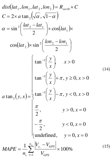
It can be defined as the average distance (Equation (14) [32]) between a random sample location and the location given by a specific localization algorithm.
b) Velocity estimation accuracy
It is measured by calculating the mean absolute percentage error (MAPE), defined by (15).
0
,
0
,
undefined
0
,
0
,
2
0
,
0
,
2
0
,
0
,
tan
0
,
0
,
tan
0
,
tan
,
tan
2
sin
cos
cos
2
sin
1
,
tan
2
,
,
,
1 1 1 2 1 2 2 2 1 1 2 2 2 2 2 1 1x
y
x
y
x
y
x
y
x
y
x
y
x
y
x
x
y
x
y
a
lon
lon
lat
lat
lat
lat
a
C
C
R
lon
lat
lon
lat
dist
earth
(14)%
100
1
1
s i n i GPS GPS e sV
V
V
n
MAPE
(15)c) Battery power consumption
It is defined as the ratio of lifetime (Equation (16)) of a specific localization algorithm,
i, to that of the benchmark scheme,Benchmark
, which performs no localization.%
100
=
lifetime
of
ratio
Benchmark i
(16)B. Experiments and Simulation Results 1) Localization
This section discusses, compares, and analyzes the localization simulation results of all of the localization algorithms mentioned above in Section IV.A.3, as well as the algorithm proposed in this paper.
a) CL
This algorithm is very simple. It does not distinguish between homogeneous or heterogeneous APs, and every AP is treated the same way. Localization is done by averaging latitude and longitude of every observed AP. This characteristic makes it more easily affected by outlier APs, as stated earlier in Section II.B.1. This makes sense that, generally, CL performs better in uniform distribution scenario. It can be seen in Figure 11 that when the number of APs are not large, localization in both scenarios are poor. As the number of APs grows, uniform scenario begins to show an edge.
Amber Red Green Amber
Red Green
0 5 25 60 Sec.
70
Fig. 11. Localization of CL.
b) WCL
Unlike CL which treats every AP the same way, WCL gives different weights to every AP. Outlier APs are weighted less than others. The experiment results are showed in Figure 12. WCL are hence less susceptible to impact of outliers. However, weight function (8) of WCL relies solely on estimated distance. Distance estimation using path loss models could be erroneous, as (2) and (9) do not take into consideration shadowing effect. Besides, in heterogeneous settings, variations also exist among APs, making distance estimation less accurate than in homogeneous settings.
Fig. 12. Localization of WCL.
c) Trilateration
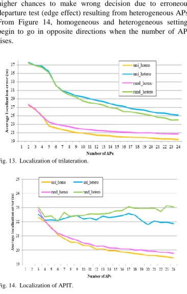
It relies heavily on transmitter-receiver separation. Nevertheless, precise transmitter-receiver separation measurement is very difficult in real life, making it highly susceptible to unfavorable effect of erroneous distance measurement. The experiment results are showed in Figure 13. Like WCL, variations among APs make the situation even worse. As for the distribution of APs, the difference between random and uniform distributions is not so significant. Trilateration works slightly better in uniform distribution.
d) APIT
As the number of observed APs is small, localization error is high due to the fact that the number of triangles formed is not large enough. To perform AIPT test, neighboring node information is used to determine node movement. With only a
finite number of neighbors, APIT could consequently make incorrect decisions. This could happen when the target is near the edge of the triangle while some of its neighbors are outside the triangle and lies further away from the others [36, 37], known as the “edge effect”. It also assumes that the longer the distance, the weaker the RSSI. Yet shadowing effect is neglected, and in heterogeneous settings, AP variations too make the departure test less accurate. These reasons exacerbate the localization result. That’s why APIT is better in homogeneous settings. As the number of APs increases, it has higher chances to make wrong decision due to erroneous departure test (edge effect) resulting from heterogeneous APs. From Figure 14, homogeneous and heterogeneous settings begin to go in opposite directions when the number of APs rises.
Fig. 13. Localization of trilateration.
Fig. 14. Localization of APIT.
e) The proposed algorithm
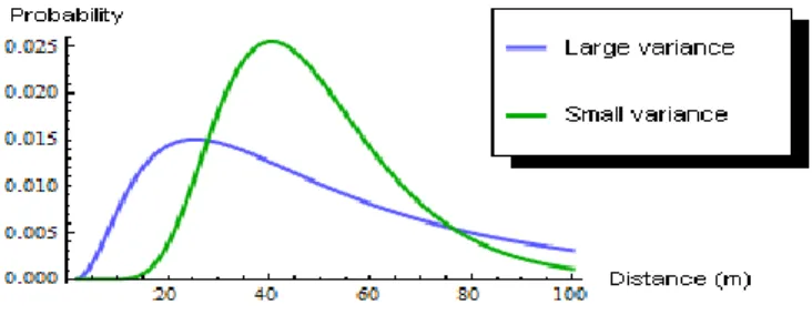
The proposed algorithm uses probability to reduce the effect of erroneous distance estimation in WCL. Suppose the log-normal model of a specific RSSI value has a high variance, distances that are relatively close or far away would have higher probabilities than if the model has small variance. However in WCL, longer distances are always weighted less than closer distances, regardless of their probabilities. In Figure 15 at both ends of PDFs, the log-normal model with large variance has higher probabilities than the one with small variance. The proposed algorithm also uses a two-phase method to narrow down anchors to a smaller area to better approximate the target’s location (Figure 16). For these reasons, the proposed algorithm can better deal with environmental variations.
Fig. 15. PDFs with the same mean and different variances.
Fig. 16. Localization of the proposed algorithm.
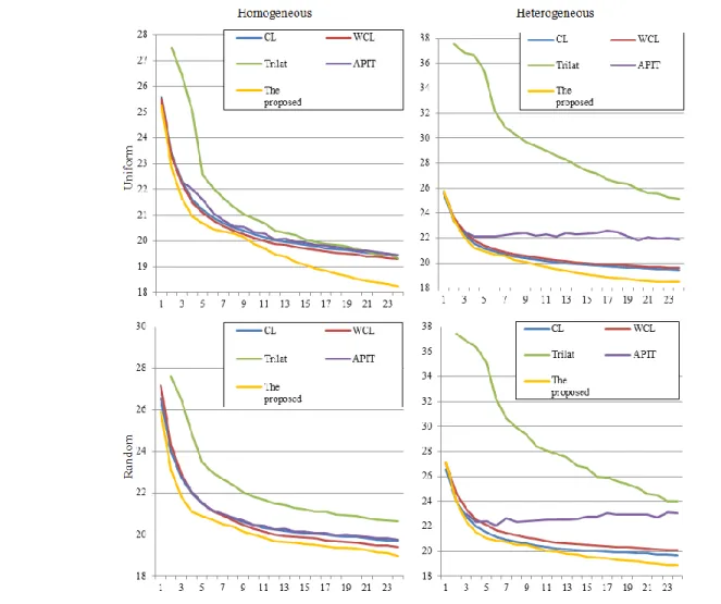
By combining Figure 11 to Figure 14 and Figure 16, an overall view of the four cases can be generated (Figure 17).
Generally speaking, trilateration itself in essence is accurate enough, but with erroneous distance estimation, its accuracy decreases as a result. APIT seems to experience turbulence in heterogeneous settings when the number of APs rises, since the chance of edge effect rises at the same time. Finally, when the number of APs is small, accuracy of CL, WCL, and the proposed algorithm is not so good. The difference between them is not so significant. As the number of APs goes up, the proposed algorithm begins to show an edge, since it can better accommodate environmental variations in all four settings.
2) Velocity Estimation
Traffic data generated by VISSIM are used to evaluate how well each Wi-Fi-based localization algorithm is at measuring vehicle velocity, and the results are shown in Table V.
TABLEV
PERFORMANCE METRIC OF VELOCITY ESTIMATION
AP AP type
Distribution Homogeneous Heterogeneous
Uniform
CL: 31.10 % CL: 31.10 %
WCL: 32.69 % WCL: 31.44 % Trilateration: 51.09 % Trilateration: 51.44 % APIT: 40.60 % APIT: 43.86 % The proposed: 28.22 % The proposed: 28.68 %
Random
CL: 36.85 % CL: 36.85 %
WCL: 35.09 % WCL: 35.15 % Trilateration: 59.59 % Trilateration: 60. 23 % APIT: 40.82 % APIT: 44.32 % The proposed: 25.39 % The proposed: 25.96 %
Precise velocity estimation relies on accurate localization. The results in Table V are similar to that of Figure 17. CL is
prone to unfavorable effect of outliers, and WCL somewhat reduces the effect experienced by CL. Trilateration and APIT are influenced by wrong distance estimation and edge effect respectively.
3) Battery Power Consumption
To test the power consumption of every localization algorithm, a program is developed and installed on a device. For the purpose of benchmarking, a case in which no localization is performed is also tested. Table VI and Figure 18 give out the experiment results.
TABLEVI
BATTERY POWER CONSUMPTION
Localization Algorithm
Sampling Frequency
Battery Lifetime
(hour : minute : second) %
1 None 2 --- 12:37:23 (45443 sec.) 100.00 % GPS 3 continuous/1 sec. 6:13:23 (22403 sec.) 49.30 % Centroid (CL) 4 continuous/1 sec. 10:54:42 (39282 sec.) 86.44 % Weighted centroid (WCL) 4 continuous/1 sec. 10: 51:45 (39105 sec.) 86.05 %
Trilateration 4 continuous/1 sec.
10: 40:49 (38449 sec.) 84.61 %
APIT 4 continuous/1 sec.
10: 32:17 (37937 sec.) 83.48 % The proposed
algorithm 4 continuous/1 sec.
10: 38:06 (38286 sec.) 84.25 %
Fig. 18. Battery power consumption of different algorithms in comparison with a benchmark scheme.
It can be told from Table VI that the proposed algorithm has a slightly shorter lifetime by as much as 3% compared with CL, WCL, and trilateration, since it requires more computation. On the other hand, compared with GPS, its lifetime is significantly longer, by about 35%. Therefore, LBSs that acquire location
1 : Lifetime of every localization approach divided by the benchmark
scheme lifetime.
2 : Benchmark scheme in which no localizations are performed. 3
: Acquire location information every second.
information frequently using GPS seems to be an inefficient solution [38].
To get a view of cost (power consumption) per unit (localization), the following calculation is performed. Suppose the battery capacity is c Joules. For the benchmark scheme, its cost 𝑏𝑁𝑜𝑛𝑒 per second is bNone=c/45443. Cost of GPS is
bGPS+bNone=c/22403. Cost of CL is bCL+bNone=c/39282. The
ratio bCL/bGPS is about 0.15250403, which means that cost per
unit of CL is about 15% of that of GPS. Similar calculations are done for other localization algorithms. The ratios of bGPS to
cost per unit of other algorithms are listed in Table VII. Apparently, using Wi-Fi for localization is less power-hungry; cost per localization is over 80% less than that of GPS.
TABLEVII RATIOS OF COST PER UNIT
Method Ratio
CL 0.15250403
WCL 0.157595441
Trilateration 0.176874116
APIT 0.192384146
The proposed algorithm 0.181766869
C. Summary
In this paper, different combinations of uniform / random distributions and homogeneous / heterogeneous APs are tested. Generally speaking, although the proposed algorithm is a little bit more complicated than CL, WCL, and trilateration, and hence consumes just a little bit more battery power, it is still far less power-hungry than GPS. In terms of localization accuracy, the proposed algorithm is robust in all four settings.
Table VIII compares different aspects of these algorithms to wrap up this section.
TABLEVIII
COMPARISON OF LOCALIZATION ALGORITHMS
CL WCL Trilateration APIT
The proposed algorithm Simplicity Good Good Fair Fair Fair
Impact of
outliers Strong Fair Fair Fair Weak Localization Fair Good Fair Fair Good
Vel. Estimation Fair Fair Fair Fair Good
Novelty Fair Fair Fair Good Good
Prevalence Good Good Good Fair --- Fig. 17. An overall view of localization algorithms in different situations
V. CONCLUSIONS AND FUTURE WORK
Conclusions are drawn in the following section. Problems that remain to be solved in the future are also discussed briefly. A. Conclusions
Nowadays, smart devices are almost ubiquitous. Their capabilities offer new opportunities for data collection. The idea of “mobile devices as probes” has begun to gain much attention. Mobility and flexibility offered by smart mobile devices are what traditional stationary sensors lack.
Power supply is a major concern for most mobile devices. GPS is one of the on-board hardware that is quite power-hungry. Therefore, this paper proposes a new localization algorithm which consumes less battery power while the localization accuracy remains acceptable. Using the proposed algorithm, it can save as much as 35% more battery power than GPS, localization error is about 18 meters, and velocity estimation error is about 25%.
While battery lifetime improves by adopting Wi-Fi-based localization schemes, localization accuracy decreases. This is a major tradeoff between accuracy and sustainability faced by many. In this paper, the purpose is to provide approximated real-time traffic information to operators, thus the more data collected, the better. Sustainability is of greater value than accuracy.
B. Future Work
The proposed algorithm adopts a “fingerprint-like” method in the model-building phase. It is assumed that radio transmission patterns are constant across time, and fluctuate with a log-normal distribution. However, in real-life situation, radio transmission patterns are not constant, and may fluctuate with other kinds of distribution, e.g. random or normal distribution, which means these models used in the localization process need to be calibrated on a regular basis to reflect current state of play and improve accuracy.
If the proposed algorithm is deployed on a metropolitan scale, the database would be very large, making it not suitable for being stored on mobile devices. Thus the localization process should be offloaded to a centralized server with fast computation speed to reduce the burden of mobile clients. Nevertheless, in this case, mobile devices are required to be connected to a wireless network in order to communicate with the server, which incurs extra communication overheads that would consume more battery power.
REFERENCES
[1] S. Li, Y. Lou, B. Liu, "Bluetooth aided mobile phone localization: a nonlinear neural circuit approach," ACM Transactions on Embedded
Computing Systems, vol. 13, no. 14, article no. 78, 2014.
[2] S. Li, B. Liu, B. Chen, Y. Lou, "Neural network based mobile phone localization using Bluetooth connectivity," Neural Computing and
Applications, vol. 23, no. 3, pp. 667-675, 2012.
[3] G. Rose, "Mobile phones as traffic probes: practices, prospects and issues," Transport Reviews, vol. 26, no. 3, pp. 275-291, 2006.
[4] S. Li, F. Qin, "A dynamic neural network approach for solving nonlinear inequalities defined on a graph and its application to distributed, routing-free, range-free localization of WSNs," Neurocomputing, vol. 117, pp. 72-80, 2013.
[5] A. Thiagarajan, L. Ravindranath, K. LaCurts, S. Madden, H. Balakrishnan, S. Toledo, J. Eriksson, "VTrack: accurate, energy-aware road traffic delay estimation using mobile phones," Proceedings of the
7th ACM Conference on Embedded Networked Sensor Systems, Berkeley,
California, USA, 2009.
[6] Wikipedia: Street canyon. [Online]. Available:
https://en.wikipedia.org/wiki/Street_canyon
[7] Taipei City Government: Taipei Free. [Online]. Available:
http://www.tpe-free.taipei.gov.tw/TPE/index_en.aspx
[8] R. Roberts, "Ranging subcommittee final report," IEEE P802.15 Working Group for Wireless Personal Area Networks, IEEE 802.15-04-0581r7, 2004.
[9] Y.C. Tseng, S.P. Kuo, H.W. Lee, C.F. Huang, "Location tracking in a wireless sensor network by mobile agents and its data fusion strategies,"
Proceedings of the 2nd International Conference on Information Processing in Sensor Networks, Palo Alto, CA, USA, 2003.
[10] Multilateration and ADS-B: Executive Reference Guide. [Online]. Available: http://www.multilateration.com/
[11] E.D. Kaplan, C.J. Hegarty, Understanding GPS Principles and
Applications, Artech House, Norwood, Massachusetts, USA, 2006.
[12] Loran-C Introduction. [Online]. Available:
http://jproc.ca/hyperbolic/loran_c.html
[13] R. Roberts, "TDOA localization techniques," IEEE P802.15 Working Group for Wireless Personal Area Networks, IEEE 802.15-04a-0572r0, 2004.
[14] N.B. Priyantha, A. Chakraborty, H. Balakrishnan, "The cricket location-support system," Proceedings of the 6th Annual International
Conference on Mobile Computing and Networking, Boston,
Massachusetts, USA, 2000.
[15] S.Y. Seidel, T.S. Rappaport, "914 MHz path loss prediction models for indoor wireless communications in multifloored buildings," IEEE
Transactions on Antennas and Propagation, vol. 40, no. 2, pp. 207-217,
1992.
[16] H. Tian, "A novel method for metropolitan-scale Wi-Fi localization based on public telephone booths," Proceedings of 2010 IEEE Position
Location and Navigation Symposium, Indian Wells, CA, USA, 2010.
[17] T. Chrysikos, S. Kotsopoulos, "Impact of channel-dependent variation of path loss exponent on Wireless Information-Theoretic Security,"
Proceedings of the 2009 conference on Wireless Telecommunications Symposium, Prague, 2009.
[18] P.C. Chen, "A non-line-of-sight error mitigation algorithm in location estimation," Proceedings of 1999 IEEE Wireless Communications and
Networking Conference, New Orleans, LA, 1999.
[19] J.S. Seybold, "Fading and multipath characterization," Introduction to RF
Propagation, pp. 163-164., Wiley, Hoboken, New Jersey, USA, 2005
[20] J.J. Egli, "Radio propagation above 40 MC over Irregular Terrain,"
Proceedings of the IRE, vol. 45, no. 10, pp. 1383-1391, 1957.
[21] C. Hurley, R. Rogers, F. Thornton, "Learning to WarDrive," WarDriving:
Drive, Detect, Defend: A Guide to Wireless Security, Elsevier,
Amsterdam, Netherlands, 2004.
[22] N. Bulusu., "GPS-less low-cost outdoor localization for very small devices," IEEE Personal Communications, vol. 7, no. 5, pp. 28-34, 2000. [23] Z. Juan, J. Hongdong, "A hybrid localization algorithm based on DV-Distance and the twice-weighted centroid for WSN," Proceedings of
2010 IEEE International Conference on Computer Science and Information Technology, Chengdu, China, 2010.
[24] J. Blumenthal, "Weighted centroid localization in Zigbee-based sensor networks," Proceedings of 2007 IEEE International Symposium on
Intelligent Signal Processing, Alcala de Henares, Spain, 2007.
[25] T.S. Rappaport, "Mobile radio propagation: large-scale path loss,"
Wireless Communications: Principles and Practice, pp. 69-74, Prentice
Hall, Upper Saddle River, New Jersey, USA, 2002.
[26] T. He, C. Huang, B.M. Blum, J.A. Stankovic, T. Abdelzaher, "Range-free localization schemes for large scale sensor networks," Proceedings of the
9th Annual International Conference on Mobile Computing and Networking, San Diego, CA, USA, 2003.
[27] R. Peng, M.L. Sichitiu, "Probabilistic localization for outdoor wireless sensor networks," ACM SIGMOBILE Mobile Computing and
Communications Review, vol. 11, no. 1, pp. 53-64, 2007.
[28] E.L. Crow, K. Shimizu, Lognormal Distributions: Theory and
Applications, CRC Press, Boca Raton, Florida, USA, 1987.
[29] M. Bolić, D. Simplot-Ryl, I. Stojmenovic, "RFID positioning techniques," RFID Systems Research Trends and Challenges, pp. 399-401, Wiley, Hoboken, New Jersey, USA, 2010.
[30] G. Keller, Statistics for Management and Economics, Southwestern Company, Nashville, Tennessee, USA, 2014.
[31] T. Bäck, Evolutionary Algorithms in Theory and Practice: Evolution
Strategies, Evolutionary Programming, Genetic Algorithms, Oxford
University Press, Oxford, UK, 1996.
[32] Wikipedia: atan2. [Online]. Available:
http://en.wikipedia.org/wiki/Atan2
[33] Wikipedia: Fitness proportionate selection. [Online]. Available:
http://en.wikipedia.org/wiki/Fitness_proportionate_selection
[34] VISSIM: Multi-Modal Traffic Flow Modeling. [Online]. Available:
http://www.vissim.de/
[35] Qon™ Hotspot Services. [Online]. Available: http://www.qon.com.tw/
[36] J.Z. Wang, "Improvement on APIT localization algorithms for wireless sensor networks," Proceedings of International Conference on Networks
Security, Wireless Communications and Trusted Computing, Wuhan,
Hubei, China, 2009.
[37] R. Stoleru, T. He, A. Stankovic, "Range-free localization," Secure
Localization and Time Synchronization for Wireless Sensor and Ad Hoc Networks, pp. 1-31, Springer, NY, USA, 2007.
[38] S. Gaonkar, J. Li, R.R. Choudhury, L. Cox, A. Schmidt, "Micro-blog: sharing and querying content through mobile phones and social participation," Proceedings of the 6th International Conference on
Mobile Systems, Applications, and Services, Breckenridge, CO, USA,
2008.
Chi-Hua Chenreceived his B. S. degree
from the Department of Management Information Systems of National Pingtung University of Science and Technology in 2007, a M. S. degree from the Institute of Information Management of National Chiao Tung University (NCTU) in 2009, and a Ph.D. degree from the Department of Information Management and Finance of NCTU in 2013. He is an associate researcher for the Internet of
Things Laboratory of Chunghwa Telecommunication
Laboratories. Furthermore, he serves as an adjunct assistant professor for the Department of Information Management and Finance of NCTU and the Department of Communication and Technology of NCTU. He has published over 140 journal articles, conference articles, and patents. His recent research interests are in the Internet of Things, Cloud Computing, Cellular Networks, Data Mining, Intelligent Transportation Systems, Network Security, Healthcare Systems, Augmented Reality, and E-Learning Systems.
Chi-Ao Lee received his M. S. degree from Department of Information Management and Finance of NCTU in 2012. His recent research interests are in Mobile Sensing, Intelligent Transportation System, and Wireless Networks.
Chi-Chun Lo received his Ph.D. degree in Computer Science from Brooklyn Polytechnic University, USA in 1987. He is a Professor in the Department of Information Management and Finance at NCTU in Taiwan. His research interests include Network Management, Network Security, Network Architecture, and Wireless Communications.
APPENDIXA:OPTIMALVALUESOFg A. The proposed algorithm
B. WCL
APPENDIXB:THE SELECTED ROAD SECTION
![Fig. 2. Impact of outliers on localization result [23]. 2) Weighted-Centroid Localization](https://thumb-ap.123doks.com/thumbv2/9libinfo/7987293.159332/3.918.512.784.298.446/fig-impact-outliers-localization-result-weighted-centroid-localization.webp)