GENERALIZED PATH-INTEGRAL FORMALISM OF THE POLARON PROBLEM AND ITS 2ND-ORDER SEMI-INVARIANT CORRECTION TO THE GROUND-STATE ENERGY

PHYSICAL

REVIE%

B VOLUME

21,

NUMBER

10

15

MAY

1980

Generalized

path-integral

formalism

of

the polaron problem

and

its

second-order

semi-invariant

correction to

the ground-state

energy

J.

M. Luttinger

Department ofPhysics, Columbia Uniuersity,

¹w

York, New York 10027

Chih- Yuan Lu

Institute ofElectronics, National Chiao Tung UniUersity, Hsinchu, Taiwan 300,Republic ofChina (Received 31January 1980)

Feynman's path-integral formalism ofthe polaron problem is generalized, by which it is easy and natural

to get the second-order perturbation result in the weak-coupling case and the Pekar result in the strong-coupling case, even in the crudest ground-state, approximation. With the harmonic approximation, the polaron energy for the whole range ofthe coupling constant is obtained, but it isfound there isatransition

at coupling constant 5.8.This generalized formalism is translationally invariant. The best self-consistent variational potential canbe determined by anumerical method. Also, in this model it is particularly easy to

estimate the second-order semi-invariant correction to the Jensen inequality. This second-order semi-invariant correction explicitly iscalculated. Itgenerates the perturbation expansion to fourth order in the weak-coupling case, and it improves Feynman's result by 0.5% for strong coupling. Discussion and suggestions forfurther study are included.

I. INTRODUCTION

The problem offinding the ground-state energy of the Frohlich polaron Hamiltonian has

a

fairly substantial literature. It

is

well known that among

all the methods, Feynman's path-integral theory gives the best ground-state energy in the overall

range of the coupling strength.

'

It is our purpose

to generalize the Feynman formalism, and we find that in the generalized theory it is much

easier

to estimate the second-order semi-invariant

cor-rection in the harmonic approximation

case.

In

Secs. II

and

III,

we present the generalized

for-malism of the path-integral theory ofthe polaron problem.

In

Sec.

IV, we apply this theory to the

ground-state energy in the ground-state approximation and harmonic approximation. In

Sec.

V, we

esti-mate the energy correction due to the

second-or-der semi-invariant term. Both numerical results

and analytic results in the extreme

cases are

giv-en. In

Sec.

VI, we summarize the results and some suggestions for further study

are

made.

II.PATH-INTEGRAL METHOD APPLIED TOTHEPOLARON

PROBLEM

p&, q&

are

the momentum and coordinate operators

of phonons of mode

j,

and the interaction terms w&(x)q&

are

(8&2vn/V)'~'[u& &(x)/k,]q&, whe.

re

u~ ~(x}is given as follows:

u,

_,

(x}=cosk

x,

u»(x)

=sink

x.

The two real waves

_{uz, (x},}

P=

1,

2, constitute

a

complete

set

when the nonzero values of k

are

re-stricted to run only over a half-space, that

is,

a space inwhich, if

a

vector k

occurs,

-k

does not

occur.

The partition function of the polaron may be written as

z e-~F

Tr(e

'")

when P

-

~,

the leading term

is

e Eo. Therefore lim _[ (1/P) lnz]=E-o,

where

_E,

is

the ground-state energy of the

polar-on. Thus we may calculate the partition function to evaluate

_E,

.

In particular, we would like to know the partition function for large P.

Using the path-integral representation, the

par-tition function is written as

The Hamiltonian of the idealized

electron-pho-non system by Frohlich is given by ~2

H=

—

+Q-,'(p,

'._{+ q,}

')+ Qw,

_.(x)q,,

J J

where we use the units

8=

m= co=1. _p,

x

are

the momentum and coordinate operators of electron,

e~~=

Tr(e

~

₎₌

_{exp — H(t)dt}

(path) 0

Here, let us define our notation clearly as follows:

We divided the time axis from 0 to P into

N+1

subintervals, each of length

_7,

i.

e.

, g= (N+

1)r,

a.nd the superscript denotes the time sequence

in-dices.

z=

dx"'

dq~"'0

—

—

—

exp

—

II

tdh

A A

B

B

x6&2&'''g

N &exp

—

7' zq& +w&

x

q

where the end point coincides with the initial point

X(N+1)₌X(0) (N+1)— (0) where We define

[dx]

=—dx ~~dx~ ~ with ~&~-&'~

I(

—₊

I)

₊e+Il&-\&'I— A A A A n =I/(ee

—1}

.

dq~ dq,

"'

dq~" dq,' '

B

B

B

B

(dx)-=dx"'[dx],

similarly for the definition of(dq&) and (Dq&), and

/

=_(2pg} & _H=—_(2pg} ~

p„=(

_)„,

exp[-(x"'

—

x"')'/2~],

1

d'„,

-=,

„„exp

_f-(q,

"'

—

_q,

'")'/k.

],

.

.

.

(2F

f)

Now let us define

Z'

by

Z

Tr(e»)

Z,

„Tr(e-»

h} '

where

H~„=

,

g(P,

'+

q,'-)-.

Ifwe integrate out the phonon coordinates

(elim-inate the phonon

oscillators),

then we obtain

Feyn-man's

result.

gdxppQ

~

/pe(x)~

gr xXOM) M)~A&~~ ~~x I

For

P

-

~,

then

I-

0,

hence we have

-Il~-l'~I

M,l,

-e

The physical motivation of our variational meth-od comes from a intuitive belief that in some sense the reaction of the lattice (phonon) system to the motions of an electron might be represented

approximately by the reactions ofa small number (hopefully, one) ofparticles coupled in some

sim-ple way to the electron and to one another. In the most simple

case,

we choose the variational Ham-iltonian

as

H„=

—

+ +v(x

—

R),

where

P,

R, and M

are

the momentum,

coordi-nate, and mass of the fictitious

particle.

We

as-sume the electron couples with the particle by a

central

force

potential

v(x-

R).

Let us carry out the variational method as

fol-lows: by adding and subtracting the term

f

eov(x(t}—

R(t})

df to the exponent of

(1),

path

inte-grating over the coordinate R, and dividing by the

partition function of

a

free particle.

Also by multiplying and dividing this expression by the

path-integral expression of the partition function of

a

system with Hamiltonian H„, therefore, we have

Z'=

DK e~

f

(DX)(DR)

exp(W+

f

v(X

-

OR)df

—

f

(x

-

ovR)df)

f

(Dx)(DR)

exp(

f',

„(x

R)df)

f

(Dx)

(DR) exp(-

f

N

v(x

-

R)df)

f

_(DR)

21

GENERALIZED

PATH-INTEGRAL

FORMALISM

OF

THE.

. .

4253 where

f{Dx}{DR}exp(-

f

eov(x

—

R)dt)

f

{DR}

as

1

v'

1

v'

ff =

--

"

--

—

'+

v(t'),

2

(M+1)

2 p

f

{DR}

is the path-integral form of the partition

function of the

free

fictitious particle,

where p

is

the reduced mass,

1/p

=

1+

1/M. Therefore, the Schrodinger equation of this

sys-tem can be separated as follows:

V=— v

xt

-Bt)dt,

0

and the average ( &„is defined by

(A)„=

f

{Dx}{DR

}Aexp(-

f

eov(x —R)dt)

f

{Dx}{DR}exp(-

f

tv(x—R)dt) ByJensen's inequality, we have

zt

=(evvv&

z

~e«v&&vz V (3) 2

V„(

(,

:

-„)

(

(,

.

t.

-,

)

V-' _ll(

_)(&((

&,c',

,((l

and the total energy E(&t, ») is given by

((t,n& &t n _2(M+

I)

tt'

(4)

The lower bound for Z'

is

given by the

right-hand side of

(3),

therefore an upper bound for

the polaron energy is

E

inZ

(V&„(IV&„

'

'=p

p"-

p'

This variational formulation

is

different from

that of Feynman's' which has used

a

specific form

of interaction

—

"harmonic interaction"

—

between the electron and the fictitious

particle.

By that

special choice, the form ofinteraction is given

explicity, and fortunately, the exact integration

over the Rvariable can be

carried

out, therefore,

in the Feynman's formulation; what remains is

the integration over the electron's coordinate

x.

In the generalized formulation, we do not specify the form ofthe interaction which can be varied to

make the inequality

(3}

as strong as possible.

The disadvantage of this formulation [as can be

seen in

_(3}]

is

our use ofJensen's inequality

twice, once

for

the path-integral average over

the electron's coordinate

x,

and the other for the

variable R. Therefore the lower bound of (3)may be weaker than that of Feynman's method ifwe

also assume the interaction

is

harmonic.

%e

will show this fact by explicit calculations in a later

section. In general, our method can be better, because we can adjust the interaction form

self-consistently, as an example, we can obtain the

Pekar result (which is better than Feynman's

re-sult in the strong coupling limit) very naturally even in the crudest approximation.

III. THE PARTITION FUNCTION OFPOLARON FORAN

UNSPECIFIED GENERAL FORM OF VARIATIONAL POTENTIAL

Inthis section, we formulate the upper bound ofthe polaron energy

for

the general form of

variational potential v(x

—R).

If the relative

coor-dinate $ and coordinate of the center of mass g

are

used, then the Hamiltonian can be expressed

Now, let us calculate Z, (V&„,and (W&

„separate-ly in order to obtain

Z'.

First,

Z

is

defined as

f{Dx}{DR}exp(-

f

eov(x- R)dt)

Z=

f

{DR}

Tr(e

N&iv}

Tr(e

e~'~

_~)

The denominator

is

the partition function of a

free

particle with mass M; this is well known

as

M

Tr(e

~

'

'"}=

_{DR}=e

«"=

_V

2mP

The partition function of the system

H„can

be

ex-pressed in _($,&})representation as (as

P-~)

v'(t

'""l

=

J

d(

f

dtt

((tt

_It

'"

l

(V&,

,

(M

()"

*

Therefore we have

Z=

_(I/p"

')e

"o.

Secondly, let us evaluate the (V&„

term.

There

are

many ways to do this; the following one

is

a

very simple one:

(vl„=(J(

(x—

R}dt)

=—

—

ln Dx DR

xexp

-A.

vx

—

Rdt

0 }isl

dx'"d

R'"

x

—

—

[lnG

(x"'

R("

x'"

R'"

(&(.v)] ex (5)

G,

(X(",

R"'x"',

R"'

~Xv)=

(X"',R'"

~e

"»

~X'",

R"')

is

the Green's function of the Hamiltonian

(p'/2) +(P'/2M) + Xv(x

—

R) beginning at

(x'", R"')

and ending

at

the same position (x&'&,R&o&).

_For

Pvery large,

G (x«» R«» x«» R&(»l&&v) ly (x&o& R&o&}loe oeo&»&

Therefore the integrand in Eq. (5)can be

calcu-lated by using perturbation theory (X=

l+

e, e

-0),

that

is,

(V)„=

P dx&o&dR&o&

=P

dx'"dR"'v

x'"

—

R'"

tt)

x'"pR'"

written as 2 E

(W)„=

—

g

g

M»

(.

u,((x(»)u,&(x&& &))

.

r, r'=0

Setting

t=(l

—f')~&

_0,

we can write this as follows:

(W)

Tr(e»o)

d P

-

t e'

Tr

e '~

"~~

e '~~zg

0

As

P-~,

we only take the ground state of the

dis-crete

level &„, and sum over the continuous quan-tum number y in the e '

"

~term in calculating

the

trace.

Ifwe also use the

fact

that

Q~,

(&),$

)~,

(&)',

t')

=

jg-g'+

&

—

&'I

=P

d'$v $ u,

(

(6)

g(n,=T-I'; _k,

h'),

₍₈₎

Last, we evaluate

_(W)„.

From Eq. (2), (W)„

is

the right-hand side of Eq. (7) is given as

M+

df B o &&u+&&('o&&(o o&

Qu+($'}u

($)u+($)u„($'}e

'"

2 2 ₀ pt v) n

the g and q' integration can be done explicitly,

t3/'

cia-

g'I

e-r.(&+&)/2t)(n-0')

_(/~2'

_erf

M+1

_p]g

_{$ j} where and, because M [2(M+

i)]"'

'

(M+()"*

"

Therefore we have the expression for

(W)„:

(w)

=

'

Q

((&

((')

dt f

)

o yg

where

+&n=&n

-

&O~

Now the t integration can be done by partial integration, and using the definition of

erf

function we have

(W)„=

&rp uo*(g')u,($}u*„($

)u„(t')

1—e

'«o'

"&

v 2p neo &q„+1

Ifwe make use ofthe Fourier transform

dk 4m

ejlr.r

IrI (2&&)'

(b'+

k'}

(9)

then

_{( W)„can}

also be expressed as

OO

]

2 oo

n

21

GENERALIZED

PATH-INTEGRAL

FORMALISM

OF

THE.

.

. 4255 where we define

b

„2=

—C(he

„+

1}'

~

Therefore, it is

clear

that every G„term

is

positive. Ifwe just take any kind ofpartial sum or a single

term, the variational bound

still

holds true, but makes the inequality weaker. Let us now summarize the results as follows:

Eo~

E„=

e, —(V)„/p

—(W)„/p

u($') u(o$) „*u($) „u($') 1—

exp[-2C(1+4&„)' 'I

₎

—

$'I]

v2p.~~o n

where we combine the

first

two terms onthe right-hand side as

(lo)

d$v $ Qp) Qp P 2P Qp

and it is noted (

W)„can

also be expressed as

(9').

2

Ep- E„=

Qp g

—

Qp

(

d(

a

lup g up g I

Since E'„is afunctional ofQpalone and the only

constraint

is

that Qp is normalized, the

station-ary condition for the best choice of v, 5E'„/bv(g) =_{0, is equivalent} to

&

E„-A

up g' 'd$' u,

(6)

=

o.

This gives at once

=

_e.

_u.

₍₍

)

(11)

From the above equation, we

see

the best

self-consistent potential

is a

Hartree-type potential.

For

the strong coupling

case,

we assume C

—

_~,

'

_Eq.

₍₁₁₎

will just reduce tothe semiclassical

theory of

Pekar.

'

According to the work ofPekar

in strong coupling

case,

the polaron

is

localized

in a Hartree-type potential well, and the polaron energy

is

then calculated by a variational method.

Pekar took the

trial

function

as

u,

(r)

= N

[1+

br+

a(br)']

e ~",

IV. GROUND-STATE APPROXIMATION AND HARMONIC

APPROXIMATION FORTHEPOLARON ENERGY

From (10)in the

last

section, it is obvious that if we take only the ground-state term (n =0) in the summation of

_(W)„,

then the right-hand side

of(10) is still an upper bound of the polaron en-ergy. Therefore we can write

then obtained the energy E'„=

-0.

1088m'.

Recently, Miyake' recalculated the

Pekar

energy by both exact numerical integration and

Pekar's

variational method. Itwas found that the

varia-tional energy

is

-0.

108504m' which

is

a

little

higher than the exact numerical quadrature value

(-0.

108513n') as it should be. Therefore, the often quoted result

-0.

1088m' of

Pekar's

varia-tional calculation

is

not quite

accurate.

But from

Miyake's work, it

is

found that

Pekar's

variation-al calculation gives an excellent approximation; the energy differs by

less

than

0.

01%&and the

error

in the wave function

is less

than 1% where the

val-ue ofthe wave function is appreciable.

For

very small coupling,

n-0,

assume

C-O,

then by expanding

(11),

we obtain an equation which

describes

an electron moving in a constant potential of magnitude

-o.

, and from

(11},

we can easily see in this limit

(n-0}

the polaron energy

is

-n,

which agrees with that of the second-order

perturbation calculation. By this variational meth-od, without any specific form of v(x

—

R), we can

now obtain the

correct

energy values in both weak and strong limiting

cases.

In order tofind the

effects of the inclusion ofall the excited

states,

we take

a

specific example ofinteraction

poten-tial

—

harmonic interaction. By this harmonic-interaction approximation, we can get the explicit results which

are

fairly good for all values

cou-pling constant.

As

a

matter of

fact

for

this particular choice of

interaction,

v(x

—

R)=—,

'Z(x —

R)',

(12)

=p-'~'~Q

~'~+

Q' —

~'

0

x(1 —

e

~))

'

'e d7,

(13)

be exactly equal to the A which appears in

Eqs.

(21)and (31)in Feynman's original paper,

'

where

A=2'

'a

1

_S,

e

'

"ds

Ix(t)

-x(s)

I

~'=

_K/M, O'=_K/p,

.

We can also obtain this result by summing up the

expression

(9')

by taking u„($)as the wave

func-tions of harmonic oscillator

as

an alternative way

to obtain the

(W)„;

we include this calculation in the Appendix.

For

the harmonic approximation,

z.

-

&~ l~(&)l~ )=&~.lp'/2t l~ )

is

given by 4Q. Therefore the upper bound of the polaron energy

is

given by

1 t

E0&

E„=

~Q

—

&Q

dt.

Wz

(

't+

[(Il' —

~')/11](1

—e

"'))"'

(14)

BE„/B~= 0, BE„/Bn=

0.

(15)

Butfrom

(14),

we can

see

that only the integral A contains

_e,

and A

is

an even function of

~,

so

the derivative ofA with

respect

to

~

is always

zero

at

~=

0,

and we can

see

from following this

that

~=

0is a point which makes A maximum.

Ifwe

set

cu=yQ and

Qt=y,

From this expression, it

is

easy to

see

that y=0 will make A maximum, therefore, the best value of &u is

zero.

Hence the energy expression (14)

can be reduced to

Unfortunately, the integral in (14)cannot be

eval-uated in closed form, so that a complete

determi-nation ofthe polaron energy requires numerical

integration.

Equation (14)has two parameters which we

varied to give the lowest energy; there we have

This means that when

n-

5.8, the best value ofQ

-0.

This can also be seen by plotting Eq. (16) di-rectly as a function ofQ for various values of

a.

It

is

found that when ca&5.

_8,

there

is

no minimum

for

E„but

the end point E„(A=O)corresponding to the least energy; for

a&5.

8, there

is a

minimum

for E„with nonzero

0

(&

0).

Plotting these

E„as

a function of n, we find

a

transition at n

=

5.

8,

that

is,

dE (a)/do,

is

not continuous at n

=

5.

8.

And for large n we can have large Q; then

Q

'

'1r-,

'

r1

Q Q

'

'

1

2ln2+C

C

is

the Euler number here. With this expression

of_A, we can determine the best choice of Q as

0

=

4 n'/9w

—

4 ln2 —

2C,

and _{hence the polaron energy}

r(1/fl)

I'(-,

'

+I/O) (16)

G

11

E„=

—

—

—

2(21n2+

C)+0

3m Qj' (19)

The condition

_(15),

BE /BA= 0, yields 3 1 r(-'.

+z)

[q(1+z) —g(2+z)

]

4

z'

I'(1+

z) vj_z

where

z= 1/Il,

and g(z)=Idldz) lnI'(z) when

z-

~

(i.e.

,

Q-O);

the condition (1V) determining n

yields

a-5.

8,

where we have used the asymptotic

relation

I'(1+

z) 1

=vz

1+

—

+,

z-~,

I'(-,"+z) 8z 1 1

y(1+z)

—q(-,

'+z)

=

—

—

+.

8z2

for

a

large coupling constant.

For

a

that

are

small,

0=0,

then (16)becomes

E„=

-a.

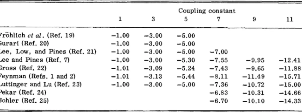
InTable

I,

a comparison ofvarious

pre-vious results about polaron energy in the range of intermediate coupling constant

a

isgiven. Here,

both Luttinger-Lu and Feynman's results

are

in the harmonic approximation. From this table, it isfound that our result

is

inferior to that of

Feyn-man'

_{s, as}

itshould be, because we have Jensen's

inequality one more time than Feynman. But it

is

known for very strong coupling that

Pekar's

energy will be lowest, and we have seen that even our

re-sult of the ground-state approximation for

a

gen-eral

form of potential will approach that of

Pekar's

result.

From this result, we know that in the strong-coupling

case,

the electron

is

trapped in

GENERALIZED

PATH-INTEGRAL

FORMALISM

OF

THE.

.

~ 4257

For

strong coupling, it reduces to

E„-

—(1/Sv)

a'-

-0.

106a'.

(21)

Comparing (21)with

(19),

we can see that the

ex-cited

states

contribute only to the "fluctuation

en-ergy"

(oforder

a ).

Therefore if we include all

the excited states in the calculation of

a

general

potential, the constant "fluctuation-energy" term

must come out

as

it does in the harmonic

approx-imation.

V. ESTIMATION OF THE ENERGY CORRECTION DUE

TOTHE SECOND-ORDER SEMI-INVARIANT

When we use the path-integral variational meth-od to evaluate the ground-state energy of the po-laron, we have assumed the Jensen inequality

&eA&

)

e(A) (22)

where A=W+t/'. However, Jensen's inequality

is

actually the

first

term of the exact

semi-invari-ant or cumulant expansion

a potential which

is

not like the harmonic

poten-tial and the contribution from the

states

other than ground state

is

not significant. Those excited

states

only contribute to the constant term instead of the

a'

term.

This can be seen clearly in the following example of harmonic interaction but

ex-cluding excited

states.

Ifwe take only the ground-state harmonic wave function in the expression

(9),

instead of taking

all the excited states into account, it

is

trivial to calculate the upper bound ofthe polaron energy [this result, of course,

is

worse than

_(16)],

and

it

is

n

n

li

n

E

~ E'„=-',_fl—

a

—

_exp

—,

I

erfc

—,

—

~]

(20) (22) and

_4E,

is

given by

nE,

=

_{-(1/p)(&wv)„-}

_{&w)„&v&„)}

.

To evaluate (24), we replace Vby i(Vin (W)„, then

(24)

(

")=

p(&A&

—,

(&A*)

—

&A)*)

—,

[(A')—3(A)((A') —(A)')—.(A&

['

")

.

Therefore, if the approximation

&eA& e(A)

is

very good, we expect that the fluctuation

(1/2})((A'& —&A)')

should be

a

small correction to the inequality

(22}.

With this second cumulant term, we no longer have the Jensen inequality, that

is,

exp[(A)+-,

'((A')

—

(A)'}]

may not be a lower bound

for

(e").

The second-order semi-invariant is

F'"=

[&(w+

v)'&-(w+ v)']

= [&w')—&w&'+2(&wv) —(w&&v))+

(v')

—&v&']

.

The second-order semi-invariant correction to

the ground-state polaron energy

is

n.

E=

-(1/2P)F'"

=

_{-(1/2P) [((W')„—}

_(W)'„)+2((WV)„—(W)„(V)„) (&v'&„-&v&„')]

=b,E~+ AE2+

EE3.

Therefore, for harmonic interaction, we

calcu-late

4E,

first,

r

_E,

=—

»

1

((v')„-

&v&'„)

TABLE

I.

Polaron energy from previous work.

Coupling constant

5 7

Frohlich eg~l.(Ref.19) Gurari (Bef.20)

Lee, Low, and Pines (Ref.21) Lee and Pines (Ref.7)

Gross (Ref.22)

Feynman (Refs.1and 2)

Luttinger and Lu (Ref.23) Pekar (Ref.24) Hohler (Bef.25)

-1.

00

-1.

00

-1.

00

-1.

00

-1.

01

-1.

01

-1.

00

-3.

00

-3.

00

-3.

00

-3.

00

-3.

09

-3.

13

-3.

00

-5.

00

-5.

00

-5.

00

-5.

30

-5.

24 544

-5.

00

-7.

00

-7.

55

-7.

43

-8.

11

-7.

36

-6.

83

-6.

70

-9.

95

-9.

65

-11.

49

-10.

72

-10.

31

-10.

10

-12.

41

-11.

88

-15.

71

-15.

00

-14.

66

-14.

33

&E,

=

--

1

—

8 (W) P ~P ~v =

t

(&())

_'~'Is(s

-)

~

_B((

~

—,

—

—

)

1+—

or 4

~

r1

_u+-,'

where

B(x,

y) is the beta function defined as

B(

)= t

'-'(1

—

)'

'dt

=-and P is defined by

(25)

Now let us concentrate on the expression (W')„ —(W)'„. From the definition of

(W')„,

it can be

ex-pressed as

a'

(W ) = ' ' ' _{dt ds dt ds} e-(tt st-l-its ss(-v 2 2 1 .1 0 (26)

lr,

-r,

I

lr,

-r,

l

Here, we may express

1/Ir,

—

_r,

I by a Fourier 1 1 transform: 1 dk

,

,

exp[ik~

(r,

—

_r,

_}),

~ 1 1

=B(x,

1—x)

[He(x)&0].

and similarly for

1/

I

r,

—

_r,

_I.

_For

this reason

we need to study

f—

:

(exp[ik

(r,

-r,

)+ik'(r,

—

_r,

_)])„

dr

e 0exp

jk r,

-r,

+ik'

_r,

_-r,

dre

o,

where

$0=——

'

—

dt — dtdg

r,

—

_r

0

The path integral in the numerator

is

of the form

N=

dr

exp S0+ f t

rtdt

(28}

where specifically

f(t)=_ik[5(t

—

_t,)

—

&(t

—

_s,

_)]

+ik'[&(t

_—t,

)

—

5(t

—

_s,

_)]

.

Following Feynman's

trick,

'

the exponent of

I

is obtained by

J=

-(k'A+

k

"B+

k'

k'D},

where

2 _Q2 2

0

M

2 _/72

(e Alto- tl+e-01st ttl s-Alt-2 ttl e-ols-s-stl) 203

hence we can write

(W')„as

B _{1 dk dk'}

(W') =

—

' ' dt ds dt ds e

"t

'& ed'(k,k')

v 2 2 1 1

4'

_y2

yI2

21

GENERALIZED

PATH-INTEGRAL

FORMALISM

OF

THE.

. .

4259

After k and k' integration, we have

Q 2

(W') =

—

dt ds dt ds e

"1

st~

"2

'2'

—

—

_tan

'

V

0

(3o)

Recall that best value of (d

for

minimum energy

is

always

0,

so in our theory the expression

for

A._,

B,

D

is

particularly simple, t1( ~t S ~) (1 e-Qltt st I_-) 1 2n

g(

~t S ~) (l e-Altt stl )-1

/e-Ql tt 321₊

-e-

lQt ₂ sl

t-e

Qltt t21-e-Qlst-ssl

)

2g

and also, (W)„

is

given, by the same

trick,

as

B B

(W)„= dt, ds,e

"1

'1',

7T o 0 k~gj

This is the expression which appeared in the Eq.

(31)

of Feynman's paper' with (d=

0.

Ifwe define 8by sin28 = D22/4n,

n2,

then we have

a'

_{-It -syl-It -s} I 8 0 1 2

In order to evaluate this expression, we need

a

theorem on multiple integration; the theorem

is:

(31)

(32)

dx„dx

x dx

2''

~j,

&x &2 ~~~

+

+'

~

d+ ₁

~-2

~1Fs

(33)

where

_F,

is

the symmetrized

F,

which is defined by

F,

=

x„x„.

_.

.

_nf,

P

the

_Q~

means to sum over all the possible permutations of the arguments of the function

_F,

that

is,

1

Fs ( IF(«lt «2t «3t ' '

')

F(«2t«tt«3t '' '

)+F(«3t

«2t «it '' ' ) ] Pls

For

our

case,

from Eq.

(26),

it can be easily found that (W')„

is

symmetric under these interchanges:

s,

—

_t„s,

—

t„and

(s„

t,

)

(s„

t,

)simultaneously. Therefore we have only three independent

expres-sions in

F„.

they

are

F(s,

t,

s,

t,

),

F(s,

s,

t,

t,

),

and

_F(s,t,

_s,

_t,

).

Hence we can write

(W')„—

(W)'„as

~2 t2 S2 tg

(W')„—

(W)'„=

—

m' 4i dt,

ds,

dt, ds,

3[F(s

t,

stt

)2F2(+s,

s,

t,

t,)+

F(s,t,

s,

t,

)],

0 0 0 0

where we assume

_t,

&

_s,

&

_t,

&

_s,

.

_{Ifwe define}

(34)

S2

—

t~—

t,

tg —

~g-t

j

we can have b

E,

"'

equal to the

first

term of

(-1/2P)((W'), —

(W)'„):

2 _{~ t} (O

e t

(l

eAt)/

3(1

eAt)/

sin8,

where sin8,=—,

'(1

—

e

"')'

'(1

—e

"')'

'.

_/2E,

'"

equals the second term of

(-1/2p)((W')

—(W)2):

2

(l e A(r+t))1/2(1

-e

A(t+tt)3/2-(35)

J.

nE(3) _{equals the} third term of

(-1/2p)((W')„—

(W)'„):

(8,

/sin8,

—

1)

dte

dte

dte

p p p

_[(I

e-G(t+t+t)}(I _e ot-)]l/2

Now, we arrive at the final result for second-order semi-invariant

correction;

the correction is

t).

E= (tlE

'+rtE

'

+

t)E,

")+

ttE2+

dE3.

(3'I }

(38)

Recalling that

for

o(& ()tc=

58,

0=

0

is

the best choice. In this

case

(0=

0),

we have t) El(t)=t)E2=_{nE3= 0,} and b.

_E,

'"

and b.

E,

"'

reduce to

AEf dt e dt e dte

~/

(2 _{t t 2(} (82/si118 1)

p p p

[(t+

t)(t+7)]"'

bE,

=

—

—

dte

dte

dte

,

—,(83/sin8'

—

1)

2 2 2

[t(t+t+t)]'

'

(39) (40) where t ((t+t

)(t+

t)

]"

'

(t

)1/2 sine,'=

(t+

t+

t)

SU16),

'=—

Therefore, for

a~

5.

8, we have

~E=

b.E&"+ b.

E,

"&=

-a'g,

where

_g

is a

pure number. We can evaluate this

pure number by numerical integration, and it

is

equal to 0.0157. Therefore,

bE=

-0.

015Va

.

Bythis value of

_0,

we can obtain the approximate energy

corrections:

From

(35), (36),

a,nd (3't),

we can have

nE(1) 1 _{~2/v t)}E(2) 1 _{~2/v t)}E(3) 1 _~2/v

This result

is

superior to both that ofHaga and

Lee and

Pine',

Haga's result does not reduce to perturbation theory to order (22(when

a

is small).

Feynman's result will reduce to that ofHaga in the weak-coupling limit. Hohler' has done the straightforward fourth-order perturbation

calcu-lation, and our result agrees with that of Hohler. Hence in this limit the cumulant

series

generates

the perturbation expansion.

Also for large o(, from (16)we know the best choice of

0

is

n-

(4/9)/)

a'.

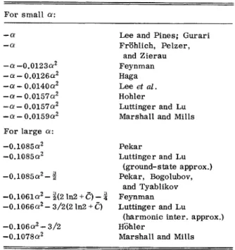
TABLE II. Polaron energy. For small n:

-~

-0.

0123~2

-o

—

0.0126~

-~

—0.0140~'

-

~

—

0.0157~'

—

~

—

0.0157~ -G.—0.0159~' For large o.

'

Leeand Pines; Gurari Frohlich, Pelzer, and Zierau Feynman Haga Lee etal,

.

Hohler Luttinger and Lu

Marshall and Mills

l

This means the coefficient of

n'

is

corrected

to

E+ ttE=

-(a'/St()(1+

—

₎

—

-0.

1066(2

.

The coefficient of

n'

is

0.

4-0.

5%lower than that

ofour previous

result.

(That

is, -I/St/:

This

is

also Feynman's

result.

) The ratio of our

cor-rected coefficient to that of

Pekar's is

0.

980.

Comparing with

0.

9'?4 which

is

the ratio of

Feyn-man's to

Pekar's,

there

is

a

small improvement. A summary ofresults of our work and that of

other authors is given in Table II(in both the weak- and strong-coupling limits). In Table III,

a

comparison between our results, with the

sec-ond order semi-invariant term added, and

Feyn-man's is given. The second-order energy

cor-rection was also

carried

out by Marshall and

Mills' in Feynman's harmonic model; their

sec-respectively.

Also, from (23)and (25), one can easily obtain

ttE2-

ct'/6)/,

tlE3-

——,

'

(2

/)t.

Therefore, in the strong-coupling limit, the

en-ergy correction

is

given by

tlE= (tt

E"'+n.

E)2'+ rtE,

"')

+rtE,

+tlE3

'

_(2'/)t. 720

-0.

1085~2

-0.

1085& -Q.lQ85+

—

23 0.1061~2 -',_(2ln2+C)

—

4

-0.

1066n —3/2(2 In2+ C)

-0.

106A2 _3/2

-0.

1078&2 Pekar Luttinger and Lu (ground-state approx.) Pekar, Bogolubov, and Tyablikov Feynman Luttinger and Lu

(harmonic inter. approx.) Hohler

GENERALIZED

PATH-INTEGRAL

FORMALISM

OF

THE.

.

. 4261 TABLEIII. Plaron energy: Comparison between Feynman's result and Luttinger and Lu's

model with second-order semi-invariant term.

Ey

-1.

012 3.44 2.55

-3.

13

4.

02 2.13

-5.

44 5.81

1.

60

-8.

11 9.85

1.

28

-11.

48 15.50

1.

15

-15.

71

0

+LL &ELL ELL++ELL 0.0

-1.

00

-0.

016

-1.

016 0.0

-3.

00

-0.

14

-3.

14 0.0

-5.

00

-0.

40

-5.

40

3.

95

-7.

36

-0.

65

-8.

01 8.45

-10.

72

-0.

84

-11.

56 14.30

-15.

00

-1.

305

-16.

31

ond-order correction

is

larger than our model of harmonic approximation,

as

it should

be.

VI. DISCUSSION AND SUMMARY

The problem of polaron has received

consider-able attention in the past

years,

many authors

conjectured that there might be

a critical

coupling constant n,

(Refs.

10and

ll};

when n exceeds this

critical

value

_(n,

-

5.

8), the wave function abruptly shrinks

(self-traps),

and the slope of

E(n}

changes discontinuously, although

E

is

still

a.continuous function of the coupling constant n.

By the path-integral representation ofpartition function, the problem of an electron moving in a

random system

is

very similar to the polaron problem. Bythis close similarity and some other arguments, there

is

a

long-standing conjecture

about the possibility of

a

"phase transition"

be-tween localized states and extended

states.

Our model

is

very similar to the path-integral method

ofFeynman which gives nondiscontinuous curve of

E'(n},

but our method indeed has the discontinuity phenomenon at

n-

5.

8.

Gross"

has suggested that the transition between the localized and extended function

is

abrupt. This abrupt change seems to

be

a

common feature ofseveral approaches. But, because Feynman's treatment

is

the most

success-ful overall theory of polaron, therefore, it

is still

an unanswered theoretical question

—

whether this

feature

is a

property of the general type

or

ifit

just

comes from approximation.

Our theory

is a

variational method; hence any

choice of

trial

potential

or

wave function wiQ give an upper bound of the exact answer. According to the previous work ofmany other authors and our

experience, the harmonic interaction potential

seems to be the most reasonable, exactly soluble potential form.

Frohlich"

has used the wave

func-tion appropriate to the lowest-energy state of an

electron in a Coulomb potential in

Pekar's

approx-imation; the wave function has the form: (P'/8w)'~'exp(=,

'P

~x~).

It

is

found the best value is when _P=5n/8 and the corresponding value for energy

is

S=

-0.

0977

n'.

In addition, Allcock' has shown in ground-state

approximation

(Pekar's

theory), "harmonic

oscil-lator's

wave function"

or

"improved Gaussian wave function" gives a better result than that of the Coulomb potential wave function. Also,

Mat-suura"

formulates the problem by path-integral

representation with an effective local Hamiltonian (Feynman's model and our model have a two-time-difference retarded effective Hamiltonian) which

is

not translationally invariant. This effective

po-tential method gives the same result

as

that

ob-tained from second-order perturbation theory.

"

Matsuura takes his choice ofeffective potential

as Coulomb potential, the results show that the Coulomb potential

is

inferior to that of harmonic potential. Clearly the calculation based on

a

har-monic potential will be reasonably satisfactory if

the exact potential and harmonic potential agree

wherever the electron's wave function

is

large,

and it

is

indeed so

as

shown by Allcock.

According to our model, the most general

ex-pression of the polaron energy

is

given by:

E,

-(,

ip'/2

i,

&

—

(W&„/P,

[p'/2p+

v($)]u„(]}=

eQ„(]),

where (W&„is given by Eq. (9)

or

Eq.

(9').

Our

formalism

is

translationally invariant. By

ignor-ing this translational invariance, our formalism

can be reduced to the same equation and energy

results

as

that of the Green's-function equation of motion analysis bg Matz et

al.

"

and the effective local Hamiltonian theory of Haken" and

Matsurra 's

Although it

is

too complicated to get the

expres-sion of the self-consistent potential in

a

closed form, we suggest some iterative procedure,

which might be very tedious, but can be done in

result will be reported elsewhere.

By the experience from the harmonic interaction

potential approximation, it

is

noticed that the

high-er

excited states contribute only to the constant

term

(n',

the fluctuation energy term); it should be

a

good

start

by

first

taking the ground-state

approximation. From this approximation, we have the self-consistent potential as the following:

(f)

—

aP2

f

dpi,

(,4')~I'

(y

Using this numerical self-consistent potential

as the starting potential, we may calculate the

ex-cited wave functions

_u„($)

from the Schrodinger equation. By these higher excited

states,

we can

estimate an improved value for (W)„by every

giv-en

p. %e

guess the self-consistent potential

ap-propriate tothe polaron problem must be like

a

Coulomb potential at large distances and like the harmonic potential in the region where the

elec-tron wave function

is large.

Using our model, it

is

easy to connect

Pekar's

result to our theory, which

is

difficult to

see

in Feynman's formulation. And it

is

shown clearly

and explicitly that the higher excited states will contribute to the fluctuation energy. This model

is not

restricted

to the harmonic approximation, although it is

a

pretty good one; in principle, any kind of

trial

potential

is

possible, and the best one certainly will be the self-consistent one. In order to

see

the order ofmagnitude of the

errors

which might occur due to the Jensen's inequality, this

model

is

particularly easy to evalute the second-order semi-invariant correction explicitly.

Because we

are

dealing with

a

three-dimensional

case,

the quantum number n actually

is a

triplet

(n„n„n~}

—= (o

),

and let us define n,+_n,+n,=p7.

Hence where we define In In fy (A1) and +00 cos(yx) e

"H,

(x}dx=7r'

'y'"e

"'~',

~00

r

+DO»n(yx)e

"H

(x)dx=

(-x

~ )y

~

e

"~

wOQ 2~ ~ ~I i~I I~II~_{t I} 2&n,t

I

„=

Jt

u„($,

)u,($._,)e'~~'~d(„ i

=1,

2,

3.

(A2)

Ifu(x

—

R)=

zK(X

—

R)',

then u(()=

.

~

=(""}"'(.

',

";:";:")

xe

'"'

"H„(v'pQ),

)H„(l

pQ),

)H„(v'

_pe),

),

where &v=4K/M, and 0=v'K/p,

.

By the

Fourier

cosine and sine transform identity, we have

APPENDIX: EVALUATION OF(W)„BYSUMMING OVER

COMPLETE STATES OFHARMONIC OSCILLATOR

From Eq.

(9'),

we write

Therefore

(W)„=

_Q

G„.

V 2p n=o

for _n, even

or

odd. We have _{defined y,}. -=k,./

v'_p.

_Q.

_So 4C dk y n,

!

n,

!

n,

!

2v'

k'(k'+

b ) (A3) (W)„=

_Q

G,

v2p

g (yP 8C 2 N ~ 2

dke~

~2 _dt

y gy n2y n3e ~~fy+"t

~2p,

&,

„„„n,

ln, in,I

Since b,

'

is proportional toN, which is the sum ofpfy &f2 ($3 we try to make it as aproduct of+] +g &3,

so

we use the identity 2, 2

21

GENERALIZED

PATH-INTEGRAL

FORMALISM

OF THE~

.

.

4263

to separate n» n»

n„by

writing b,

'

=4C'(dg,+1)=4C AN+

4C',

(t)

=

'

"*

_u

tan-"'*--"*&» &

"&"""-"*""

"~"'1

w v2p 0 0 Jt.

J.

Qp 8+2 ttO tto 3

dke"

~' '

'

_"@[exp(-y

_et

_«~'}]

V2p. ~ o o j=1 oP 8C' 1 ewe

«

e

'dt

dk exp — ~ t+ k' v 2p. ~ o o 2ttA

oP,

2p.a,

"'

eWC

4C2 dt

(1+

2ttAt—

e~e

«)'

»

'

(A4) Therefore,

(~)"-

_A

'

et

"=

_{nQ dt}

(&o't+[(A'

—

td')IA](1

—

e

«))'

'

=A(A,

~).

(A5)

T. D. Schultz, Phys. Rev. 116,526 (1959).

~R. P. Feynman, Phys. Rev. 97, 660(1955).

3From our work inharmonic approximation, itcan be

seen that, in the strong-coupling case, M ~ will

give the lowest ground-state energy.

4S.Pekar,

J.

Phys. 10, 347 (1946); Zh. Eksp. Teor. Fiz. 19,796 (1954).

S.

J.

Miyake,

J.

Phys. Soc. Jpn. 38, 181 (1975).

~H. Haga, Prog. Theor. Phys. 11,449 (1954).

~T. D. Lee and D. Pines, Phys. Rev. 92, 883(1955). G. Hohler, Nuovo Cimento 2, 691(1955).

SJ.

T.

Marshall and

L.

R. Mills, Phys. Rev. B2, 3143 (1970).

' D. Larsen, Phys. Rev. 172, 967(1968).

' _{D. Larsen, Phys. Rev. 187, 1147 (1969).}

'

_E.

_P.

_{Gross, Ann. Phys. (New York) 8, 78(1959).}

' _{H. Fribhlich, Adv. Phys. 3, 325(1954).}

' G. R.Allcock, Adv. Phys. 5, 412 (1956).

SM. Matsuura, Can.

J.

Phys. 52, 1 (1974).

'6M.

_E.

_Engineer and N. Tzor, Phys. Rev. B 5, 3029 (1972).

' _{D. Matz and}

_B.

_{C. Burkey, Phys. Rev. B3, 3487}

(1971).

H. Haken, Z. Phys. 147, 323(1957).

~

H. Fr5hlich, H. Pelzer, and S. Zienau, Philos. Mag.

41,221 (1951).

2_{M. Gurari, Philos. Mag. 44, 329 (1953).}

T.

D. Lee,

F.

Low, and D. Pines, Phys. Rev. 90, 297(1953).

E.

P.

Gross, Phys. Rev. 100, 1571(1955). Here we estimate the ground-state energy by

har-monic approximation.

24S.

_I.

_{Pekar, Unterschlngen} Uber Die Elecktronen Theoric der Kristalle (Akademie, Berlin, 1954). ~G. H5hler, Z. Phys. 140, 192 (1955).