先進分散式製造規劃與控制之研究(3/3)

行政院國家科學委員會專題研究計畫 成果報告

先進分散式製造規劃與控制之研究(3/3)

計畫類別： 個別型計畫

計畫編號： NSC93-2213-E-002-010-

執行期間： 93 年 08 月 01 日至 94 年 10 月 31 日

執行單位： 國立臺灣大學工業工程學研究所

計畫主持人： 周雍強

報告類型： 完整報告

報告附件： 國際合作計畫研究心得報告

處理方式： 本計畫可公開查詢

中 華 民 國 94 年 10 月 12 日

行政院國家科學委員會專題研究計畫成果報告

先進分散式製造規劃與控制之研究 (3/3)

計畫編號：

93-2213-E-002-010

執行期限： 93 年 8 月 1 日至 94 年 7 月 31 日

主持人：

周雍強

[email protected]

國立台灣大學工業工程所

一、中英文摘要

供應鏈的管理架構是分散式的，但是必 須講求整體控制。一方面，供應鏈的經營權 責分佈在各節點，因此供應鏈所要求的製造 服務品質有別於過去一貫注重的節點內的工 廠效率，供應鏈管理的挑戰在於如何促進節 點間有效協同合作。另一方面，供應鏈也是 一個系統，對外在的變化會有所反應，因此 必須講求整體控制，以提昇服務的可靠度。 供應鏈之中經常發生產品設計、製程改 進、需求變動等方面的動態事件，這些事件 往往對供應鏈的生產造成很大的衝擊。本計 畫第三年建構供應鏈的動態控制模式，這個 模式以動態事件為輸入資料，調節各生產節 點的生產決策，並作為風險控管的運算基礎。 關鍵詞：供應鏈管理、供應鏈控制 Abstract

The management architecture of supply chain s is largely distributed rather than centralized. Because the responsibility and authority is distributed over the supply chain nodes, enhancing inter-nodal collaboration is a major challenge to improving the quality of manufacturing services offered by the supply chains. On the other hand, supply chains are a system, which will respond to external impetus. System control is also essential to improve the reliability of service quality.

Keywords : supply chain management,

constraint modeling and reasoning, integrated scheduling

二、計畫緣由與目的

由於半導體供應鏈有複雜多樣的問題， 本計畫以半導體供應鏈為研究的對象，探討 系統控制。半導體供應鏈的範圍涵蓋晶圓製 造、晶圓針測、晶粒封裝、以及產品測試。 供應鏈每個階段都有多個平行工廠，形成一 個網路。而晶圓廠內也有供應鏈的現象，一 個晶圓廠一般分為數個製程模組區，各區自 為一個工場，並且由部門經理負責管理，各 製程模組甚至其中的機群間有前後製程的關 係，從排程與派工的角度，也是供應鏈的節 點關係。另外，企業內有多個規劃與排程部 門，包括生產規劃、總排程、作業排程、維 修排程等等，這些功能的整合也是供應鏈管 理的重要議題。本計畫的研究重點是供應鏈 分散式規劃與控制，所謂的供應鏈將包含這 些廠間、部門間、功能間 的供需關係。以下 先說明問題背景與協同式規劃的必要性。 供應鏈節點之間的關係通常錯綜複雜， 形成動態的網路，每個節點的行為是受自我 績效利益與目標所影響，橫跨部門或工場的 整合工作，由於受到組織界限的牽制，統制 式的整合往往很難有好的效果，協同式整合 由於兼顧到效益創造與合理分享，在許多情 況比較可行。 另一方面，供應鏈也是一個系統，對外 在的變化會有所反應，因此必須講求整體控 制，以提昇服務的可靠度。供應鏈之中經常 發生產品設計、 製程改進、需求變動等方面 的動態事件，這些事件往往對供應鏈的生產 造成很大的衝擊。例如，半導體製造過程經 常發生良率的突發工程問題， 當製程與機台 出現問題，在製品批量會扣留在原地，因而 造成在製品在供應鏈中的流動停滯，而一旦 這些工程問題得到解決，扣留的在製品批量 得到放行，又再度改變在製品流動。 這樣的 變化對後階工場的生產效率會造成衝擊。

2

Figure 1 is a conceptual diagram for the relationship between the information of dynamic events, production units of the supply chain, and production decisions. Demand shocks, engineering problems and

manufacturing yields are common examples of dynamic events that could result in significant changes to the capacity requirements in the supply chains. For stakeholders of the supply chain, whenever such an event occurs, it is important to assess its impact on the capability of supply and order fulfillment. Such analysis will typically result in several scenarios of changes in capacity requirements. T he changes are marginal demand (E(t)) beyond nominal production. In this figure, the supply chain is made up of a number of nodes (k ) and the source of dynamic events is indexed as node 0.

Node 1 (k=1) Node 2 (k=2) marginal demand Capacity (µ1) Capacity (µ2) Fk E(t) r1 r2 Events in demand, engineering, manufacturing (Node 0) Analysis of capacity needs Control

Figure 1: A dynamic system model of supply chains

In a supply chain it is not necessarily beneficiary to set the production rate at the capacity or to independently set the production rate at individual nodes. The marginal demand could overload some nodes of the supply chain and thus affect the overall performance of the supply. Coordinated efforts at the nodes might have to taken in order to cope with the

dynamic events. In the conceptual framework of Figure 1, the loading decision (r_k) at each

node determine the utilization of the resources

and flow time ( F_k). There have been many

studies on the modeling of factory operation. However, it is very rare to find models that integrate the operation of multiple production units to address a common problem.

研究目的

There are two major research issues for the dynamic system of Figure 1: (1) modeling of the production behavior of the nodes and (2) designing a mechanism that link up production decisions at the nodes. The goal of this project is to develop control methods to integrate node

0 with the supply chain nodes so that the performance of the whole system can be enhanced and predicted.

三、研究方法

In this project, we will use channel inventory as an example of dynamic events to illustrate our approach to dynamic c ontrol of the supply chain. In the semiconductor supply chains, channel inventory includes those stockpiles of microchips in foundry manufacturers, IDMs, electronic

manufacturing service companies (EMS) and distributors. C hanges in channel inventory level are a good indicator of imminent market demand. Fresh information of excessive inventory is a trigger for revising ordering or production decisions throughout the demand and supply chains.

One problem addressed by this project can be described as follows. The customers of the supply chain are the initiators of inventory adjustment. Figure 2 illustrates three example inventory adjustment curves, which are named aggressive, moderate and conservative policies for their respective rates of bringing the

inventory back to the norm. Two research questions can be posted. The first question is that given any adjustment trajectory, can it be supported by the workload and capacity profile of the supply chains at the time? Another question is related to the production decision of the manufacturers: what are the best

coordinated production decisions to meet the goal of an adjustment trajectory?

0% 20% 40% 60% 80% 100% 120% 0 1 2 3 4 Time Adjustment Aggressive Moderate Conservative

Figure 2: Representative policies for excess inventory adjustment In the project we have developed a discrete-time dynamic control model for the dynamic system of Figure 1. The inventory adjustment policy determine s the arriving

process of incremental demand (i.e., urgent demand) at the supply end of the chain.

Let ~I₀(t) be the ideal inventory level and )

( 0 t

I be the actual inventory level in the

channels. The excessive inventory is the difference between the actual and ideal inventory levels. Let t₀be the time that

inventory adjustment is triggered. The

adjustment is to be made over a certain horizon

of Ω time periods. The marginal demand to the

supply chain can be expressed as:

(

( ) ~ ( )

)

)

(t I₀ t₀ I₀ t₀ E =−α_tp −

where the superscript p indexes the various

policies and p

t

α represents a faction of the

total adjustment to be made in time t. In the dynamic system, the control variables are the release rate rk,,t at each

production unit. Define W_k

( )

t as the work-in-process at shop k at time t. Suppose that there are two production units in the chain. The following two equations relate the material flow, release rates and marginal demand over all time periods t.

) ( ) ( ) ( ) 1 ( _{1 1 1} 1 t W t r t F Et W + = − − + … (1) ) ( ) ( ) ( ) 1 ( _{2 2 2 1 1} 2 t W t r t F r t F W + = − − + − … (2)

Suppose that at time t= 0, channel inventory level is I0(t), work-in-process information is

Wk(t), and initial production rates rk,t are

known. Considering that different inventory adjustment policies p will have different marginal capacity requirements at the time t, the state of supply chains at time t can be described by an augmented state variable x(t).

T F t r t r t r F t r t r t r t W t W t x()=[ 1(), 2(), 1(),1(−1),...,1( − 1),2(),2( −1),..., 2( − 2)]

State components I0(t), W2(t), and control

variable rk,tare real numbers. Based on

equations (1) and (2), the dynamics of the supply chains is given as:

φ +             +       + +             +             − = + () 0 0 0 1 ) 1 ( ) 1 ( 0 0 0 0 0 0 ) ( 0 0 0 0 0 0 1 0 0 0 1 ) 1 ( 2 1 _Et t r t r D D t x C C B A A t x

[ ]

  − = + = = otherwise F j a a A _{j j} , 0 1 , 1 , ₁ 1 1

[ ]

  − = + = = otherwise F j b b B _{j j} , 0 1 , 1 , ₁ 2 1

[ ]

   = + = = otherwise j i c c C _{ij ij} , 0 1 , 1 ,

[ ]

   = = = otherwise i d d D _{i i} , 0 1 , 1 , ₁ 1

Since the objective is to identify the stress point in the supply chain, the objective function can be set to minimize excess workload (as measured by a given threshold percentage of the capacity level).

( )

[ ]

(

)

      − ≡ = ∑ = ∑= > 2 1 1 , 0 max ,0 min , k T t kt k k r W t x v Min Z t k µ β

where β is a threshold value. The solution can

be found by a dynamic programming procedure.

四、結論與成果

The dynamic control model described above is a tool that can be used in controlling the production operation of the supply chain. This is demonstrated using a generic chain of two nodes in Figure 3. Suppose there are three inventory adjustment policies which are called aggressive, moderate and conservative, respectively, each with certain fraction of inventory adjustment in each time period (Table 1). Shop 1 Shop 2 F₁= 3 Weeks F₂ = 5 Weeks E(t) policy -5k k/month 72 = λ 54 80 1 1 = = W µ 90 5 . 77 2 2 = = W µ Shop 1 Shop 2 F₁= 3 Weeks F₂ = 5 Weeks E(t) policy -5k k/month 72 = λ 54 80 1 1 = = W µ 90 5 . 77 2 2 = = W µ

Figure 3: A generic chain of two nodes Table 1: Example of three adjustment policies

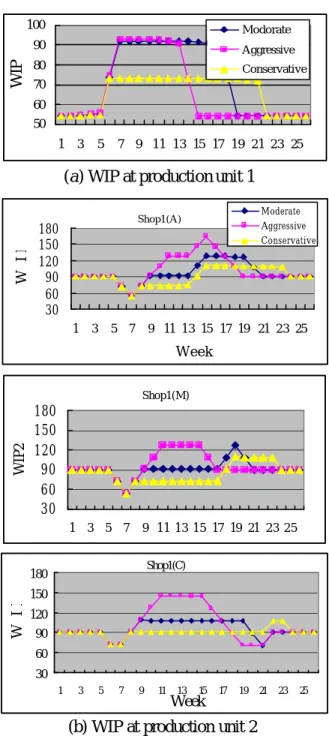
0.25 0.25 0.25 0.25 Conservative 0 0.34 0.33 0.33 Moderate 0 0 0.5 0.5 Aggressive Policy (p) 4 3 2 1 Time (t) Fraction α(t) 0.25 0.25 0.25 0.25 Conservative 0 0.34 0.33 0.33 Moderate 0 0 0.5 0.5 Aggressive Policy (p) 4 3 2 1 Time (t) Fraction α(t) Figure 4 shows the WIP levels of the two production units over the planning horizon for each of the adjustment policies. The resultant WIP levels at shop 1 are different for the three policies (Figure 4-a). For each WIP level trajectory at shop 1, the three polices at shop 2 will generate a distinct WIP trajectory (Figure

4 4-b). 50 60 70 80 90 100 1 3 5 7 9 11 13 15 17 19 21 23 25 WIP Modorate Aggressive Conservative

(a) WIP at production unit 1

Shop1(A) 30 60 90 120 150 180 1 3 5 7 9 11 13 15 17 19 21 23 25 Week W IP2 Moderate Aggressive Conservative Shop1(M) 30 60 90 120 150 180 1 3 5 7 9 11 13 15 17 19 21 23 25 WIP2 Shop1(C) 30 60 90 120 150 180 1 3 5 7 9 11 13 15 17 19 21 23 25 Week W IP2

(b) WIP at production unit 2 Figure 4: Utilization Fluctuations during

Inventory Adjustment

By using β₁=1.1andβ₂ =1.5, the total cost for the nine WIP trajectory combinations at shops 1 and 2 are shown in Figure 5. The best paths are for shop 1 to take the

conservative policy and for shop 2 to follow either the moderate or conservative policy. Since many performance measur es of production are directly related to system

utilization, this dynamic control model provides a link between dynamic event information and future performance.

A M C A M C M A C 0 A M C 42.4325 57.15 0 54.975 10 0 164.187 0 0 32.125 0 SHOP 1 SHOP2 A A MM C A M C A A MM CC M M A A CC 0 0 A M C A A MM CC 42.4325 57.15 0 54.975 10 0 164.187 0 0 32.125 0 SHOP 1 SHOP2

Figure 5: the benefits of coordinating release rates

REFERENCES:

[1] Hsieh, T. Y., H Y Huang, Y C Chou and S C Chang, “Managing Supply Chain by Using Channel Inventory Information,” Proc. 3rd International Conference on Modeling and Analysis of Semiconductor Manufacturing, Singapore, Oct. 6-7, 2005, pp. 332-338.