國
立
交
通
大
學
多媒體工程研究所
碩 士 論 文
利用雙鏡面環場影像攝影和超音波感測技術作
戶外自動車學習與導航之研究
A Study on Learning and Guidance for Outdoor Autonomous
Vehicle Navigation by Two-mirror Omni-directional Imaging
and Ultrasonic Sensing Techniques
研 究 生:黃政揆
指導教授:蔡文祥 教授
利用雙鏡面環場影像攝影和超音波感測技術作
戶外自動車學習與導航之研究
A Study on Learning and Guidance for Outdoor Autonomous
Vehicle Navigation by Two-mirror Omni-directional Imaging
and Ultrasonic Sensing Techniques
研 究 生:黃政揆 Student:Jheng-Kuei Huang
指導教授:蔡文祥 Advisor:Wen-Hsiang Tsai
國 立 交 通 大 學
多 媒 體 工 程 研 究 所
碩 士 論 文
A ThesisSubmitted to Institute of MultimediaEngineering College of Computer Science
National Chiao Tung University in partial Fulfillment of the Requirements
for the Degree of Master
in
Computer Science
June 2010
Hsinchu, Taiwan, Republic of China
利用雙鏡面環場影像攝影和超音波感測
技術作戶外自動車學習與導航之研究
研究生:黃政揆
指導教授:蔡文祥 博士
國立交通大學多媒體工程研究所
摘要
隨著電腦視覺技術之發展,立體式攝影機逐漸受到歡迎。本研究使用一種新 型的立體攝影機與新的引導技術來建製一台機械導盲犬,用以帶領使用者在人行 道環境中行走。 在本論文中,我們提出一個新型立體式攝影機的設計方法與公式,讓使用者 可以輕易地設計一支立體式攝影機。接著提出一種基於空間對映法的攝影機校正 方法來校正此立體式攝影機。基於同軸旋轉不變性質,我們提出適用於此新型立 體攝影機的立體資訊之計算方法;不同於其他計算方法,本系統無須將環場影像 轉換為全景影像即可計算影像對映點與立體資訊。此外自動車在行走中累積的機 械誤差會影響導航時的計算,對此我們亦提出一個誤差校正模型以解決問題。接 著我們發展一動態調整相機感光值的方法與一動態調整參考值的方法,來適應環 境中不均勻亮度的問題。 我們在本系統中以人行道之路延石作為行走時的特徵點,提出了兩種擷取特 徵點的方法。當自動車進行學習時,系統計算特徵點的立體值,找出行走時的方 向與距離並據以自動行走,同時自動紀錄與分析路徑點,以建立環境地圖。此外 我們亦提出一種人機互動的技術,允許使用者在任何時候都可以手勢控制自動 車,此時系統將關閉計算特徵點的程序,並進行盲走之程序。 當自動車進行導航模式時,我們亦提出一種分析串列超音波訊號的方法,使 自動車能配合使用者的速度,調整自身行走速度並帶領使用者於環境中行走。接著我們提出一種改良的閃避障礙物之方法與自動車座標計算之方法,讓自動車能 在環境中判斷障礙物的高度,並進行閃避。最後我們提出相關的實驗結果證明本 系統的完整性與可行性。
A Study on Learning and Guidance for Outdoor
Autonomous Vehicle Navigation by Two-mirror
Omni-directional Imaging and Ultrasonic Sensing
Techniques
Student: Jheng-Kuei Huang
Advisor: Wen-Hsiang Tsai
Institute of Multimedia Engineering, College of Computer Science
National Chiao Tung University
ABSTRACT
With the progress of development in computer vision technologies, 3D stereo cameras nowadays become more popular than in the past. In this study, a new imaging device and new guidance techniques are proposed to construct an autonomous vehicle for use as a robot guide dog navigating on sidewalks to guide the blind people.
A general formula for designing a new stereo camera consisting of two mirrors and a single conventional projective camera is proposed. People can use the formula to design other stereo cameras easily. Then, a calibration technique based on a so-called pano-mapping technique for this type of camera is proposed. Using an autonomous vehicle to navigate in the environment, the incrementally increasing mechanical error is a big problem in the experiment. A calibration model based on the curve fitting technique is proposed to correct such errors. Also, a 3D data acquisition technique using the proposed two-mirror omni-camera based on the rotational invariance property of the omni-image is proposed. The 3D data can be obtained
directly without transforming taken omni-images into panoramic images.
The autonomous vehicle is designed to follow the curb line of the sidewalk using the line following technique. In the path learning procedure, two methods are proposed to extract the curbstone feature points. If there exits no curbstone features or the features are hard to extract, a new human interaction technique using hand pose position detection and encoding is proposed to issue a user’s guidance command to the vehicle. To adapt the adopted image processing operations to the varying light intensity condition in the outdoor environment, two techniques, called dynamic exposure adjustment and dynamic threshold adjustment are proposed. To create a path map, a path planning technique is proposed, which reduces the number of the resulting path nodes in order to save time in path corrections during navigation sessions.
In the navigation procedure after learning, there may exits unexpected obstacles blocking the navigation path. A technique using a concept of virtual node is proposed to design a new path to avoid the obstacle. Finally, to allow the vehicle to guide a blind person to walk smoothly on a sidewalk, a sonar signal processing scheme is proposed for synchronization between the speed of the vehicle and that of the person, which is based on computation of the location of the vehicle with respect to the person using the sonar signals.
A series of experiments were conducted on a sidewalk in the campus of National Chiao Tung University. And the experimental results show the flexibility and feasibility of the proposed methods for the robot guide dog application in the outdoor environment.
ACKNOWLEDGEMENTS
I am really appreciative of the kind guidance, discussions and support from my advisor, Dr. Wen-Hsiang Tsai. Something Dr. Tsai gave me is not only aspects of development of this thesis, but also attitude of relationship between people and encouragement of facing to problems.
Thanks also given to all classmates in Computer Vision Laboratory in the institute of Computer Science and Engineering at National Chiao Tung University. They have their own personalities which I have to learn with them- careful derivative thinking of Mr. Bo-Jhih You and Mr. Guo-Fong Yang, great programming skills of Miss. I-Jen Lai and Miss. Mei-Hua Ho, positive attitude of Miss. Pei-Hsuan Yuan and Mr. Chih-Hsien Yao, and friendly of Che-Wei Lee who shares his experience with me and inspires me when I lost my emotions in the institute interval.
Finally, I extend my profound thanks to my family for their love, care and support. I cannot acommplish this dissertation without them.
CONTENT
ABSTRACT ...iii
CONTENT ...vi
LIST OF FIGURES ...ix
LIST OF TABLES...xiii
Chapter 1
Introduction ...1
1.1 Motivation... 1
1.2 Survey of Related Works ... 2
1.2.1 Types of guide dog robot ... 2
1.2.2 Types of omni-camera ... 3
1.2.3 Types of stereo omni-camera ... 4
1.2.4 Different learning and guidance methods for autonomous vehicles ... 5
1.3 Overview of Proposed System... 6
1.4 Contributions of This Study... 7
1.5 Thesis Organization... 9
Chapter 2
Proposed Ideas and System Configuration... 10
2.1 Introduction... 10
2.1.1 Idea of proposed learning methods for outdoor navigation... 10
2.1.2 Idea of proposed guidance methods for outdoor navigation... 12
2.2 System configuration... 13
2.2.1 Hardware configuration ... 13
2.2.2 System configuration ... 17
Chapter 3
Design of a New Type of Two-mirror Omni-camera ... 23
3.1 Review of Conventional Omni-cameras... 23
3.1.1 Derivation of Equation of Projection on Omni-image ... 24
3.2 Proposed Design of a Two-mirror Omni-camera ... 26
3.2.1 Idea of design ... 26
3.2.2 Details of design... 27
3.2.3 3D data acquisition ... 34
Chapter 4
Calibrations of Vehicle Odometer and Proposed
Two-mirror Omni-camera ... 37
4.1 Introduction... 37
4.2 Calibration of Vehicle Odometer... 37
4.2.1 Idea of proposed odometer calibration method... 37
4.2.3 Proposed curve fitting for mechanical error correction... 38
4.2.4 Proposed calibration method... 41
4.3 Calibration of Designed Two-mirror Omni-camera ... 42
4.3.1 Problem definition ... 43
4.3.2 Idea of proposed calibration method ... 43
4.3.3 Proposed calibration process... 44
4.4 Experimental Results... 51
Chapter 5
Supervised Learning of Navigation Path by
Semi-automatic Navigation and Hand Pose Guidance... 56
5.1 Idea of Proposed Supervised Learning Method ... 56
5.2 Coordinate Systems ... 57
5.3 Proposed Semi-automatic Vehicle Navigation for Learning ... 58
5.3.1 Ideas and problems of semi-automatic vehicle navigation... 58
5.3.2 Adjustment of the exposure value of the camera ... 59
5.3.3 Single-class classification of HSI colors for sidewalk detection 62 5.3.4 Proposed method for guide line detection ... 64
5.3.5 Line fitting technique for sidewalk following... 69
5.3.6 Proposed method for semi-automatic navigation... 72
5.4 Detection of Hand Poses as Guidance Commands ... 73
5.4.1 Idea of proposed method for hand pose detection... 73
5.4.2 Use of YCbCr colors for hand pose detection... 74
5.4.3 Proposed hand shape fitting technique for hand pose detection . 77 5.4.4 Proposed dynamically thresholding adjustment... 80
5.4.5 Proposed hand pose detection process... 81
5.5 Proposed Path Planning Method Using Learned Data ... 82
5.5.1 Idea of path planning ... 82
5.5.2 Proposed path planning process ... 83
Chapter 6
Vehicle Guidance on Sidewalks by Curb Following... 85
6.1 Idea of Proposed Guidance Method ... 85
6.1.1 Proposed synchronization method of vehicle navigation and human walking speeds ... 85
6.2 Proposed Obstacle Detection and Avoidance Process... 88
6.2.1 Proposed method for computation of the vehicle position ... 88
6.2.2 Detection of obstacles... 90
6.2.3 Ideas of proposed method for obstacle avoidance... 93
6.2.4 Proposed method for obstacle avoidance... 96
Chapter 7
Experimental Results and Discussions... 99
7.2 Discussions ...104
Chapter 8
Conclusions and Suggestions for Future Works... 107
8.1 Conclusions...107
8.2 Suggestions for Future Works...108
LIST OF FIGURES
Figure 1.1 FOV’s of different camera types [7]. (a) Dioptric camera. (b) Conventional
camera. (c) Catadioptric camera. ... 4
Figure 1.2 Flowchart of proposed system... 8
Figure 2.1 The color of curbstone at a sidewalk in National Chiao Tung University. .11 Figure 2.2 (a) The Arcam-200so produced by ARTRAY co. (b) The lens produced by Sakai co. ... 15
Figure 2.3 A prototype of the proposed two-mirror omni-camera. ... 18
Figure 2.4 The omni-images taken by the two-mirror omni-camera which is placed at different elevations of angles. (a) Image taken when the optical axis of the camera is parallel to the ground. (b) Image taken when the optical axis of the camera is placed at an angle of 45o with respect to the ground... 18
Figure 2.5 The proposed two-mirror omni-camera is equipped on the autonomous vehicle. (a) A side view of the autonomous vehicle. (b) A 45o view of the autonomous vehicle... 19
Figure 2.6 Pioneer 3 is the vehicle we use in the study [19]. ... 19
Figure 2.7 The notebook ASUS W7J we use in the study. ... 20
Figure 2.8 Architecture of proposed system. ... 22
Figure 3.1 A conventional catadioptric camera. (a) Structure of camera. (b) The acquired omni-image [7]. ... 23
Figure 3.2 The possible shapes of reflective mirrors are used in omni-cameras [7]... 24
Figure 3.3 An optical property of the hyperbolic shape. ... 24
Figure 3.4 Relation between the camera coordinates and the image coordinates... 26
Figure 3.5 The desired omni-image. ... 28
Figure 3.6 A simplified modal from Figure 3.4. ... 29
Figure 3.7 The light ray is reflected from the biggest radius from the mirror. ... 33
Figure 3.8 The simulation images. ... 33
Figure 3.9 Computation of 3D range data using the two-mirror omni-camera. (a) The ray tracing of a point P in the imaging device. (b) A triangle in detail (part of (a))... 34
Figure 3.10 The frontal placement of the two-mirror omni-camera. ... 36
Figure 3.11 A side view of Figure 3.8. ... 36
Figure 4.1 The floor of Computer Vision Laboratory in National Chiao Tung University. (a) Using the lines on the floor of the laboratory to assist the experiment. (b) Pasting the tape to form an L-shape on the floor. ... 39
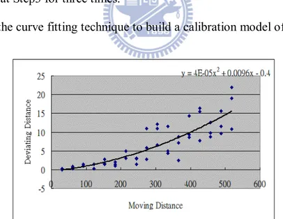
Figure 4.3 The calibration model of the odometer built by the curve fitting technique.
... 42
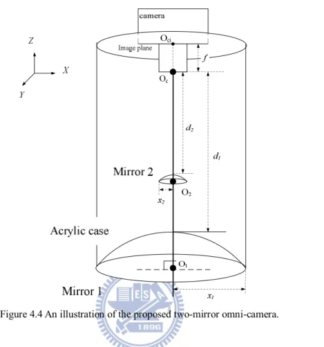
Figure 4.4 An illustration of the proposed two-mirror omni-camera. ... 45
Figure 4.5 The first step of the proposed calibration method. (a) Make sure the enclosure is parallel to the Mirror 1. (b) Make sure the lens center is match on the mirror center. ... 47
Figure 4.6 The property, rotation invariance of the omni-camera. ... 48
Figure 4.7 Experimental results of mirror base parallelism test. (a) An omni-image captured by the two-mirror omni-cameras not parallel (b) An omni-image captured by the two-mirror omni-cameras after being made parallel. ... 49
Figure 4.8 The illustration of the learning process of the pano-mapping method. ... 51
Figure 4.9 The graphical representation identifies the elevation angles ... 53
Figure 5.1 An illustration of the learning procedure. ... 57
Figure 5.2 The coordinate systems used in this study. (a) The image coordinate system. (b) The vehicle coordinate system. (c) The vehicle coordinate system. (d) The camera coordinate system... 59
Figure 5.3 The relationship between the exposure of the camera and the average of the intensity of the input image. (a) The distributed data. (b) The distributed data with a fitting line. ... 61
Figure 5.4 The HSI color model [23]. ... 62
Figure 5.5 Experimental results of extracting curbstone features. (a) An input image. (b) The curbstone features extracted by the hue channel. (c) The curbstone features extracted by the hue and saturation channels. ... 65
Figure 5.6 Two extraction windows used to detect guide line. (a) A extraction window used for detection of lateral direction. (b) A extraction window used for detection of frontal direction. ... 67
Figure 5.7 The result of detecting the curbstone features in the experimental environment. ... 67
Figure 5.8 The guide line (the red dots) extracted by the proposed method. ... 68
Figure 5.9 Finding the corresponding point for the feature point. (a) The scanning order. (b) The experimental results. ... 71
Figure 5.10 An illustration of the proposed scheme to refine the range data. (a) Fitting the range data. (b) Computing the distance from each data to the line. (c) Refined result... 71
Figure 5.11 The dangerous (damage) zones along the guide line. ... 72
Figure 5.12 Four detection regions with different vehicle commands... 75
Figure 5.13 The YCbCr color space model [25]. ... 76
Figure 5.15 The detection of the human hand using blue-difference and red-difference components. (a) The result of the Cb component. (b) The result of the Cr
component. (c) The intersection of the Cb component and the Cr
component. ... 77
Figure 5.16 The result image of the human hand detection. (a) The noises are detected as the human hands. (b) The correct detection. ... 80
Figure 5.17 A map created in the experimental environment. ... 82
Figure 5.18 A map is created with the path planning process... 84
Figure 6.1 An illustration of the navigation procedure... 86
Figure 6.2 The illustration of sonar arrays. (a) The fore sonar array of the vehicle. (b) The fore and aft sonar arrays [19]... 86
Figure 6.3 The illustration of sonar arrays. (a) The fore sonar array of the vehicle. (b) The fore and aft sonar arrays [19] (cont’d). ... 87
Figure 6.4 The range of a sonar sensor in detecting obstacles... 87
Figure 6.5 An illustration of the defined regions used for synchronizing the vehicle speed with that of the user. ... 87
Figure 6.6 An illustration of the proposed algorithm. (a) The vehicle is at Pi. (b) The vehicle is at Pi+1.... 90
Figure 6.7 positions of extraction windows... 92
Figure 6.8 The obstacle features. ... 92
Figure 6.9 The outline feature points of the obstacle. (a) The result image with both portions of feature points. (b) The result of the upper feature points of (a). (c) The result of the lower feature points of (a)... 93
Figure 6.10 An illustration of the avoidance method. (a) The avoidance method proposed in Chiang and Tsai [21]. (b) A situation in an assumption. ... 94
Figure 6.11 An illustration of a virtual node in the proposed method... 96
Figure 6.12 To avoid an obstacle at guide lines. (a) The obstacle is at the straight guide line. (b) The obstacle is at a corner... 96
Figure 7.1 The experimental environment... 99
Figure 7.2 A curbstone appearing in front of the vehicle. (a) A captured image. (b) An image obtained from processing (a) with extracted feature points. ...100
Figure 7.3 A curbstone appearing at the lateral of the vehicle. (a) A captured image. (b) An image obtained from processing (a) with extracted feature points. ...101
Figure 7.4 A resulting image of hand pose detection. (a) A user instructing the vehicle by hand. (b) The human hand detected in a pre-defined region. ...102
Figure 7.5 Two navigation maps. (a) A map created before path planning. (b) A map obtained from modifying (a) after path planning...103
Figure 7.7An experimental result of an obstacle avoidance process. (a) An obstacle in front of the vehicle. (b) A side view of (a). (c) The vehicle avoiding the obstacle. (d) A side view of (c). (e) Obstacle detection result using a
captured image...105 Figure 7.8 A light pollution on the omni-image...106
LIST OF TABLES
Table 2.1 The hardware equipments we use in this study... 14
Table 2.2 The specification of Arcam-200so. ... 15
Table 2.3 The specification of lens... 15
Table 2.4 Specification of the vehicle Pioneer 3... 20
Table 2.5 Specification of ASUS W7J... 20
Table 3.1 The parameters of the proposed two-mirror omni-camera obtained from the design process. ... 33
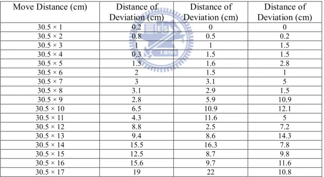
Table 4.1 The data of the experiment of building the calibration model of the odometer. ... 42
Table 4.2 The proposed calibration table... 51
Table 4.3 The coefficients of fr... 52
Table 4.4 Locations (X, Y, Z) of the calibration landmarks and the estimated location (estX, estY, estZ)... 53
Table 4.5 Error ratios in location estimations with calibration landmarks... 55
Table 5.1 The vehicle commands table. ... 75
Table 5.2 The definition of the counter used for different commands. ... 75
Table 5.3 Different type of the path nodes... 83
Chapter 1
Introduction
1.1 Motivation
According to the report of Taiwan Guide Dog Association in 2010, if all blind people in Taiwan want to have their own guide dogs, at least the following problems will arise in our society:
1. there are fifty thousand blind people, but only twenty-eight guide dogs in Taiwan till now;
2. it costs at least one million NT dollars to train a guide dog;
3. besides problems about quantity and funds, it is unavoidable to spend much time to get guide dogs acquainted with blind people;
4. problems about personality between guide dogs and blind people also have to be solved.
We believe that technology is used to solve problems that people encounter, so in this thesis study it is desired to solve the problem of guide dog shortage by constructing a robot guide dog with new visual sensing equipments and new autonomous vehicle guidance techniques. Specifically, we try to design a new type of camera, called two-mirror omni-directional camera, (or just two-mirror omni-camera), and use it to capture stereo images of the environment. Also, we desire to use an autonomous vehicle to implement the robot guide dog and develop new methods to carry out the autonomous vehicle guidance work. To achieve these goals in this study, at least we have to solve the following problems:
3. how to design intelligent methods for the vehicle to perform specified actions after learning?
We will describe the methods we propose in this study for solving these problems in the subsequent chapters. In the following sections, a survey of related works is given in Section 1.2. An overview of the proposed system is described in Section 1.3. And some contributions of this study are reported in Section 1.4.
1.2 Survey of Related Works
In this section, we categorize existing research results related to this study as follows. A survey of the types of guide dog robot is given in Section 1.2.1. A survey of the types of omni-camera used as the eye of the dog is given in Section 1.2.2. A survey of the types of stereo omni-camera for use in image taking and 3D information inference is given in Section 1.2.3. Finally, a survey of different learning and guidance methods for autonomous vehicles (used as robots) is given in Section 1.2.4.
1.2.1 Types of guide dog robot
According to the problems mentioned previously, developing a guide dog robot is a popular research topic recently. We may categorize the research results of this topic into four types roughly as follows.
1. Use of electronic travel aids:
Some researchers tried to use electronic sensors to help the blind people to avoid obstacles. Borenstein and Ulrich [1] developed a device using sonar sensors to detect obstacles. The user pushes the device ahead of him/ herself to perform this function. When the device detects any obstacle, it uses sound or vibration to let the user know the existence of obstacles around.
In this type, researchers developed navigable devices equipped on the user’s body to detect obstacles. Sun and Su [2] developed a vision-based aid system which uses two webcams worn on the head of the user to detect obstacles and sends the information back to the user by sound.
3. Use of mobile robots as guide dogs:
Based on powerful computability of modern computers, some researchers developed vision-based mobile robots to detect obstacles, do path planning, localize current spots, and navigate in various environments. Some of such developments in the industry were found in [3][4].
4. Use of white canes:
The white cane is a device that most of the blind people use to assist walking. Guo [5] developed a digital white cane which used five sonar sensors and an embedded system to detect obstacles and water on the road.
1.2.2 Types of omni-camera
Contrary to conventional cameras, omni-cameras have larger fields of view (FOV’s), and may be used to take images with less blind areas and more visual information. Omni-cameras can be categorized into two types according to their optics architecture, namely, dioptric and catadioptric. The structures of these two types of camera are shown in Figure 1.1. A well-known example of dioptric omni-cameras is the fish-eye camera [6]. It captures incoming light directly which goes to the camera sensors through the lens.
Contrary to the dioptric camera, a catadioptric camera captures incoming light from a reflective mirror. The mirror of the catadioptric camera can be made of different shapes, like conic, parabolic, hyperbolic, etc. [8]. If all light rays pass through a common point in the reflective mirror, the catadioptric camera is
categorized as of the single-view-point (SVP) type; otherwise, as of the non-single-view-point (non-SVP) type [9].
(a) (b) (c)
Figure 1.1 FOV’s of different camera types [7]. (a) Dioptric camera. (b) Conventional camera. (c) Catadioptric camera.
1.2.3 Types of stereo omni-camera
Many different combinations of mirrors and cameras have been proposed to construct omni-cameras. According to the literature, Ukida et al. [10] used two vertically-aligned omni-cameras to construct a stereo camera system and proposed a method to calibrate it. The epipolar lines are constrained to vertical lines. Zhu [11] used two horizontally-aligned omni-cameras to construct another type of stereo camera system. While using two or more cameras to construct a stereo camera system, keeping the mutual parallelism or alignment of the optical axes of the multiple omni-cameras is a difficult problem to be solved. Therefore, in the recent years, some other researchers tried to avoid this problem by using a single camera with multiple mirrors to construct a stereo camera system. He et al. [12] used an omni-directional stereo camera of this type to detect objects. The author used mirrors of the same shape to construct the omni-camera. Yi and Ahuja [13] used a convex mirror and a concave lens to construct a stereo omni-camera with a single camera. Jang et al. [14] used two hyperbolic mirrors to construct a stereo camera system in which one mirror surface is
FO V FO V FO V
faced to the other mirror surface. A common point of all these researches is the trial to design new camera structures to solve the problem of optical-axis parallelism or alignment.
1.2.4 Different learning and guidance methods for
autonomous vehicles
About the procedure of learning which should be conducted before autonomous vehicle navigation, many methods have been proposed to control the autonomous vehicle to learn the environment. Chen and Tsai [15] and Wang and Tsai [16] proposed algorithms for controlling the autonomous vehicle manually to record navigation paths in the environment. Tsai and Tsai [17] and Chen and Tsai [18] used the color of clothes as features and used a person following technique to guide the autonomous vehicle to learn the path in the indoor environment. Chen and Tsai [19] used ultrasonic sensors to detect the feet of a person with fuzzy control techniques to guide the autonomous vehicle to learn the path in the indoor environment. Wang and Tsai [20] proposed a method using an elliptic skin model to detect human faces. The model defines a region of skin color described by the YCbCr color space to describe
the features of human faces.
In the procedure of navigation, the mobile robot navigates in environments by path maps which are learned in the procedure of learning. Avoiding dynamic obstacles is a major task in the navigation procedure. Tsai and Tsai [17] proposed a guidance method using sequences of ultrasonic signals in an indoor environment. They analyzed the ultrasonic signals which were detected during navigation and guided people on the learned path. Chiang and Tsai [21] proposed a method to avoid dynamic obstacles. After detecting an obstacle, the robot computes two passing paths to the next path node. And it decides which path to go by comparing the distances from the
current position to the next path node through the two passing paths.
1.3 Overview of Proposed System
The goal of this study is to design a vision-based robot guide dog in outdoor environments using an autonomous vehicle. We summarize the work into four major stages in the following and show a flowchart of the system processes in Figure 1.2.
1. Design of proposed two-mirror omni-camera:
At the beginning, a new two-mirror omni-camera is designed. The shapes of the two mirrors are made of a hyperbolic shape. The design of the two-mirror omni-camera is based on an optical property of the hyperbolic shape light rays, after being reflected by either mirror, pass through one focus point of the hyperbola and then to the other focus point definitely. We equip the camera on the autonomous vehicle. This phenomenon of the light ray reflection satisfies the SVP property mentioned previously, which is less complicated than the non-SVP property.
2. Calibration of proposed two-mirror omni-camera and the autonomous vehicle:
In this stage, we proposed a method to construct space-mapping tables to calibrate the proposed two-mirror omni-camera based on the pano-mapping method proposed by Jeng and Tsai [22]. The detail of the camera design and the calibration procedure will be introduced in Chapter 3 and Chapter 4, respectively. The next step in this stage is to calibrate the autonomous vehicle we use as the guide dog. The problem we have to solve is that the odometer in the vehicle we use to record the position and the turning angle of the vehicle at specified spots is not precise enough. A curve fitting technique is proposed to correct this problem which is also introduced in Chapter 4.
3. Learning procedure:
In the procedure of learning which is necessary before the vehicle can be navigated, we adopt the technique of line following for vehicle guidance. The line to follow by the vehicle is the curb of the road in the outdoor environment. And to detect the along-road curb line, we use the color of the curbstone and describe it by its HIS color features in the omni-image captured by the proposed two-mirror omni-camera. Furthermore, a hand position detection technique is proposed to guide the autonomous vehicle to learning navigation paths. Finally, brightness fluctuation in the outdoor environment is also a problem to be solved in this study. We propose two methods, called dynamic threshold adjustment and dynamic exposure adjustment, to reduce the influence of the problem on the imaging analysis result for use in vehicle guidance. The detail is introduced in Chapter 5.
4. Navigation procedure:
In Chapter 6, we will introduce the techniques proposed in this study for use in the navigation procedure. We use ultrasonic sensors and design a human-foot detection algorithm to synchronize the speed of the autonomous vehicle with the person guided by the robot dog (the vehicle itself). We also proposed a method adapted from a method, called goal-directed minimum-path following, proposed by Chiang and Tsai [21] to avoid dynamic obstacles encountered in the navigation stage.
1.4 Contributions of This Study
Some contributions made by this study are listed in the following.A new type of stereo camera, called two-mirror omni-camera, is designed in this study.
omni-camera to generate a relation between the image coordinates and the world coordinates.
St art
Design the two -mirror om ni-ca mera
Navig ating an d synchronizing spe ed
with t he use r
En d Calib ra te the two -mirror om ni-ca mera
Learn path m ap s sem i-automatica lly
Figure 1.2 Flowchart of proposed system.
2. A method is proposed to correct accumulated mechanical errors of the vehicle position and direction resulting from long-time autonomous vehicle navigation and inaccurate odometer readings.
path semi-automatically using a technique of hand position detection proposed in this study.
4. A technique is proposed to adjust image thresholds dynamically in outdoor environments under different intensity for the purpose of object detection in omni-images.
5. Twotechniques are proposed to extract the guiding (curb) line of the sidewalk in the environment.
6. A method is proposed to calculate the height and depth of in-road objects for the vehicle to avoid dynamic obstacles.
7. A foot detection method is proposed to synchronize the speed of the autonomous vehicle with the guided person by ultrasonic sensing techniques.
1.5 Thesis Organization
The remainder of this thesis is organized as follows. In Chapter 2, the proposed ideas of the study and the system configuration are introduced. In Chapter 3, the design of the proposed two-mirror omni-camera is described. In Chapter 4, the proposed techniques for calibration of the two-mirror omni-camera and correction of the mechanical error of the autonomous vehicle are described. In Chapter 5, we describe the supervised learning method for generating the navigation path map in the outdoor environment. In Chapter 6, an adaptive method used to avoid dynamic obstacles and a technique used to synchronize the vehicle speed with the user’s are described. In Chapter 7, experimental results and discussions are included. Finally, conclusions and some suggestions for future works are given in Chapter 8.
Chapter 2
Proposed Ideas and System
Configuration
2.1 Introduction
In this chapter, we will introduce the major ideas proposed in the thesis study. In Section 2.1.1, we will introduce the main ideas of the proposed learning method for outdoor navigation and use some figures to illustrate our ideas. In Section 2.1.2, we will describe the main ideas of the proposed guidance method. To develop the system of this study, we designed a two-mirror omni-camera and equipped it on an autonomous vehicle. The entire hardware configuration is described in Section 2.2.1. The software configuration and the system architecture are presented in Section 2.2.2.
2.1.1 Idea of proposed learning methods for outdoor
navigation
The main purpose in the learning procedure is to create a path map and then instruct the vehicle to navigate according to the map in the outdoor environment. As mentioned in our survey, many methods have been proposed to guide the autonomous vehicle for learning navigation maps. Different from those methods which essentially conduct learning manually, we use special features in the environment to guide the autonomous vehicle to learning the path map semi-automatically.
In addition, in this study we use the color of the curbstone at the sidewalk, as the example shown in Figure 2.1, in the outdoor environment to guide the autonomous vehicle for the purpose of learning a path map. If the color is similar to the ground color of the sidewalk or if no special color appears on the curbstone in the
environment, the autonomous vehicle will not know how it should go in the procedure of learning. Therefore, it is desired to propose another method to handle these conditions. A new approach we use in this study consists of several major steps as follows.
1. Allow the user aside the vehicle to touch the transparent plastic enclosure of the omni-camera at several pre-selected positions on the enclosure which represent different meanings of commands for guiding the vehicle.
2. Detect the hand touch position from the omni-image taken when the hand is put on the camera enclosure.
3. Determine the command from the detected hand position.
4. Instruct the vehicle to conduct navigation according to the command.
In addition, when navigating in outdoor environments, the vehicle often encounters the problem of varying light intensity in the outdoor environment which has a serious influence on the image analysis work. Our general idea to solve this problem is to dynamically adjust the camera exposure value as well as the image threshold value used in the hand detection process just mentioned.
Figure 2.1 The color of curbstone at a sidewalk in National Chiao Tung University.
We use seven major steps to accomplish the learning procedure as described in the following.
1. Decide whether it is necessary to adjust the camera exposure value and the image threshold values for use in image analysis.
2. Use the hue and saturation of the HSI color space to detect sidewalk curbstone features.
3. Detect the edge between the sidewalk region and the curbstone region. 4. Compute the range data of the guide line formed by the curb using the
detected edge.
5. Instruct the vehicle to perform actions to follow the guide line.
6. Detect hand positions in the taken image to guide the vehicle if necessary. 7. Execute the procedure of path planning to collect the necessary path nodes
and record them in the learning procedure.
2.1.2 Idea of proposed guidance methods for outdoor
navigation
In this study, the autonomous vehicle is designed to guide the blind people to walk safely on the sidewalk environment which is learned in the learning procedure. To accomplish this, we may encounter at least two difficulties as follows.
The first is whether the vehicle knows the existence of the user who follows the autonomous vehicle. In several studies, some developers design a pole to let the user hold it and follow the guide robot. But if the user releases the pole, the robot would not know that the user is behind. To solve this problem, we propose a method using ultrasonic sensors to synchronize the speed of the autonomous vehicle with that of the blind.
Another difficulty is that some dynamic obstacles may block the navigation path of the autonomous vehicle. In Chiang and Tsai’s method [21], they used a 2D projection method to compute the depth distance and the width distance of the
obstacle, and generated the minimum avoidance path from the current position to the next path node. Because they used only one camera to capture the image in the environment, the vehicle cannot know the height distance of the obstacle. If the obstacle is not flat and blocks the navigation path, it could go forward instead of avoiding the obstacle. In our study, we use the proposed two-mirror omni-camera to detect path obstacles and so can get the range data of the obstacle to solve this problem.
In addition, we propose an adaptive collision avoidance technique based on Chiang and Tsai’s method [21] to guide the vehicle to avoid dynamic obstacles after detecting the existence of them.
We use seven major steps to accomplish the procedure of navigation as described in the following.
1. Decide whether it is necessary to adjust the camera exposure value and the threshold value for use in image analysis.
2. Compute the distance from the vehicle to the user by the ultrasonic sensors equipped on the vehicle to synchronize their speeds.
3. Detect the guide line.
4. Localize the position of the vehicle with respect to the guide line. 5. Detect the existence of any dynamic obstacle.
6. Plan a collision-avoidance path.
7. Navigate according to the collision-avoidance path to avoid the obstacle if any.
2.2 System configuration
All hardware equipments we use in the study are listed in Table 2.1. There are an autonomous vehicle, a laptop computer, two reflective mirrors designed by ourselves, a perspective camera, and a lens. We will introduce them in detail as follows.
Table 2.1 The hardware equipments we use in this study.
To construct an omni-camera, it is desired to reduce the size of the perspective camera so that its projected area in the omni-image can be as the small as possible (note that the camera appears as a black circle in an omni-image). We use a projective camera of the model ARCAM-200SO which is produced by ARTRAY Co. to construct the proposed two-mirror omni-camera, and the used lens is produced by Sakai Co. The picture and the specification of the camera and the lens are listed in Figure 2.2, and Table 2.2 and Table 2.3, respectively The camera size is 33mm × 33mm × 50mm with 2.0 M pixels. The size of the CMOS sensor is 1/2 inches (6.4mm × 4.8mm). The specifications of the camera and the lens are important, because we use the parameters in the specifications to design the proposed two-mirror omni-camera, and we will introduce the design procedure in detail in Chapter 3.
Before explaining the structure of the proposed two-mirror omni-camera, we illustrate the imaging system roughly in Figure 2.3. The light rays from a point P in the world go into the sensor of the camera both though the reflective mirrors and the center of the lens (the blue line and the red one in the figure).
Equipments Product name Produced corporation
Autonomous vehicle Pioneer 3 MobileRobots Inc.
Computer W7J ASUSTek Inc.
Two reflective mirrors Micro-Star Int'l Co.
Camera ARCAM-200SO ARTRAY co.
(a) (b)
Figure 2.2 (a) The Arcam-200so produced by ARTRAY co. (b) The lens produced by Sakai co. Table 2.2 The specification of Arcam-200so.
Max resolution 2.0 M pixels
Size 33mm × 33mm × 50mm
CMOS size 1/2” (6.4 × 4.8mm)
Mount C-mount
Frame per second with max resolution 8 fps
Table 2.3 The specification of lens.
Mount C-mount
Iris F1.4
Focal length 6-15mm
We equipped the two-mirror omni-camera on the autonomous vehicle in such a way that the optical axis of the camera is parallel to the ground originally. Figure 2.4(a) shows the omni-image taken by the two-mirror omni-camera when it was affixed on the vehicle to be parallel to the ground. The regions in the omni-image drawn by red lines are the overlapping area reflected by the two mirrors. We can see that part of the omni-image reflected by the bigger mirror is covered by that reflected by the small mirror, and the overlapping area is so relative smaller. To compute the range data of objects in the world, each object should be captured by both mirrors. And if this overlapping area is too small, the precision of the obtained range data will
become worse.
To solve this problem, it is observed that a front-facing placement of the two-mirror omni-camera with its optical axis parallel to the ground reduces the angle of incoming light rays and so also reduces the overlapping area of the two omni-images taken by the camera. To enlarge this overlapping area, we made a wedge-shaped shelf with an appropriate slant angle and put it under the camera to elevate the angle of the optical axis with respect to the ground, and an omni-image taken with the camera so installed is shown in Figure 2.4(b). We can see that the overlapping area becomes relatively larger now. The proposed two-mirror omni-camera system with its optical axis elevated to a certain angle and affixed on the autonomous vehicle is shown in Figure 2.5.
The autonomous vehicle we use is called Pioneer 3 which was produced by MobileRobots Inc., a picture of it is shown in Figure 2.6, and its specification is listed in Table 2.4. Pioneer 3 has a 44cm × 38cm × 22cm aluminum body with two 16.5cm wheels and a caster. The maximum speed of the vehicle is 1.6 meters per second on flat floors, the maximum speed of rotation is 300 degrees per second and the maximum degree to climb is 25o. It can carry payloads up to 23 kg. The autonomous vehicle carries three 12V rechargeable lead-acid batteries and if the batteries are fully charged initially, it can run for 18 to 24 hours continually. The vehicle is also equipped with 16 ultrasonic sensors. A control system embedded in the vehicle provides many functions for developers to control the vehicle.
The laptop computer we use in this study is ASUS W7J which was produced by ASUSTeK Computer Inc. We use an RS-232 to connect the computer and the autonomous vehicle and use a USB to connect the computer and the camera. A picture of the notebook is shown in Figure 2.7, and the hardware specification of the laptop is listed in Table 2.5.
2.2.2 System configuration
To develop our system, we use Borland C++ Builder 6 with updated pack 4 on the operating system Windows XP. The Borland C++ Builder is a GUI-based interface development environment (IDE) software and it is based on the C++ programming language. The company, ARTAY, provides a development tool of the camera, called Capture Module Software Developer Kit, to assist developers to construct their systems. The SDK is an object-oriented interface which is based on the Windows 2000 and Windows XP systems, and written in many computer languages such as C++, C, VB.net, C#.net and Delphi. The company, MobilRobots Inc., provides an application programming interface (API), called ARIA, for developers to control the vehicle. The ARIA is an object-oriented interface which is usable under Linux or Windows system in C++ programming language. We use the ARIA to communicate with the vehicle to control the velocity, heading and some navigation settings of it.
Reviewing of the design process of the proposed system, there are four major steps as described in the following.
1. We design a two-mirror omni-camera and equip it on the autonomous vehicle.
2. We propose a calibration method based on Jeng and Tsai’s method [22] to calibrate the camera and propose a calibration method using a curve fitting technique to correct the odometer values available from the autonomous vehicle system.
Figure 2.3 A prototype of the proposed two-mirror omni-camera.
(a) (b)
Figure 2.4 The omni-images taken by the two-mirror omni-camera which is placed at different elevations of angles. (a) Image taken when the optical axis of the camera is parallel to the ground. (b) Image taken when the optical axis of the camera is placed at an angle of 45o with respect to the ground.
(a) (b)
Figure 2.5 The proposed two-mirror omni-camera is equipped on the autonomous vehicle. (a) A side view of the autonomous vehicle. (b) A 45o view of the autonomous vehicle.
Table 2.4 Specification of the vehicle Pioneer 3
Size 44cm 38cm 22cm
Max speed 1.6 m / sec
Max degree of climbing 25o
Max load 23 kg
Figure 2.7 The notebook ASUS W7J we use in the study.
Table 2.5 Specification of ASUS W7J. System platform Intel Centrino Duo
CPU T2400 Duo-core with 1.84 GHz
RAM size 1.5 GB
GPU Nvidia Geforce Go 7400
HDD size 80 GB
3. In the learning phase, we record environment information and conduct the path planning procedure to get necessary path nodes. We then detect the color of the curbstone, and use the result as well as a line fitting technique to compute the direction and position of the autonomous vehicle. We also use a method to find the user’s hand positions to command the autonomous vehicle.
4. In the navigation phase, the autonomous vehicle can guide the person in the environment that has been learned in the learning phase. We design a method to synchronize the vehicle speed with that of the user. Then, we use the proposed two-mirror omni-camera to compute the range data of obstacles and use a method to avoid dynamic obstacles.
We divide our system architecture into three levels and show our concept in Figure 2.8. Several hardware controlling modules are in the base level. Imaging process techniques, pattern recognition techniques, some methods for computing 3D range data, and some data analysis techniques are in the second level. The highest level shows our main processing modules based on techniques and knowledge in the second level.
The road detection module is used to detect the guide line (the curb) along the sidewalk to guide the autonomous vehicle. The hand position detection module is used to detect the user’s hand positions to guide the autonomous vehicle when necessary in the learning procedure. The speed synchronization module adjusts the vehicle speed dynamically to synchronize with the human speed. The position processing module is used to record the learned paths in the learning phase and to calculate the vehicle position in the navigation phase. And the obstacle avoidance module handles the avoidance process to avoid collisions with obstacles after the autonomous vehicle detects the existence of dynamic obstacles in the navigation procedure. We will show more complete ideas and describe these techniques in more detail in the following chapters.
Chapter 3
Design of a New Type of Two-mirror
Omni-camera
3.1 Review of Conventional
Omni-cameras
A conventional omni-camera is composed of a reflective mirror and a perspective camera. An example is shown in Figure 3.1(a), and an omni-image captured by the omni-camera is shown in Figure 3.1(b). We can see that the omni-image has larger FOV’s with the aid of a reflective mirror, compared with those taken with the traditional camera. The shape of the mirror may be of various types such as hyperbolic, ellipsoidal, parabolic, circular, etc. An illustration is shown in Figure 3.2. More about the design principle of the two-mirror omni-camera we use in this study will be described in the next section.
Figure 3.1 A conventional catadioptric camera. (a) Structure of camera. (b) The acquired omni-image [7].
Figure 3.2 The possible shapes of reflective mirrors are used in omni-cameras [7].
3.1.1 Derivation of Equation of Projection on
Omni-image
The two-mirror omni-camera used in the study is constructed by two reflective mirrors made of the hyperbolic shape and a camera with a perspective lens. Here, we use an omni-camera with a mirror made of the hyperbolic shape to show the derivation of the equation of image projection first. An important optical property of the hyperbolic-shape mirror is illustrated in Figure 3.3, which says that when a light ray goes through one focus point F1 of the hyperbolic shape at a space point P which is on
the hyperbolic curve, the ray will be reflected to the other focus point F2 definitely.
Figure 3.3 An optical property of the hyperbolic shape.
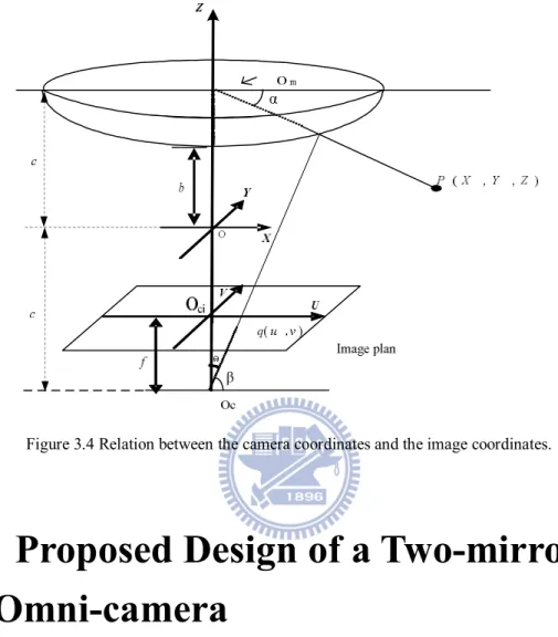
We use this property of the hyperbolic shape to construct the omni-camera we need in this study. The image projection phenomenon of the omni-camera is shown in Figure 3.4 and two coordinate systems, namely, the camera coordinate system (CCS)
and the image coordinate system (ICS), are used to illustrate the principle of the imaging process. Based on the property mentioned previously, the light ray of a point P(X, Y, Z) in the CCS first goes to the center of the mirror Om, then is reflected by the
mirror to the center of the lens Oc by the hyperbolic mirror surface, and finally is
projected on the image plane to form the image point q(u, v) in the ICS. To satisfy this property of the hyperbolic shape, the optical axis of the perspective camera and the mirror are assumed to be alignedsuch that the omni-camera becomes to be of the SVP type.
The point O is taken to be the origin in the CCS which is also the middle point between the two focus points Om and Ocof the hyperbola, where Om, which is also the
center of the base of the hyperbolic-shaped mirror, is located at (0, 0, -c); and Oc is +
located at (0, 0, c) in the CCS. The hyperbolic shape of the mirror of the omni-camera can be described by the following equation:
1 2 2 2 2 b Z a R , R X2 Y2 (3.1)
where a and b are two parameters of the hyperbolic shape, and
2 2
c a b (3.2)
is the distance to the focus point Om. The projection relationship between the CCS and
the ICS can be described [7] as:
2 2 2 2 2 2 2 ( ) ( )(Z ) 2 (Z ) Xf b c u b c c bc c X Y , 2 2 2 2 2 2 2 ( ) ( )(Z ) 2 (Z ) Yf b c v b c c bc c X Y , (3.3)
where f is the focal length of the camera.
Figure 3.4 Relation between the camera coordinates and the image coordinates.
3.2 Proposed Design of a Two-mirror
Omni-camera
3.2.1 Idea of design
The conventional non-stereo camera can only take images of single geometric planes, and cannot be used to get 3D range data, including the depth, width, and height information of scene points, compared with the stereo camera. While using two or more cameras to construct a stereo camera system, keeping the mutual parallelism or alignment of the optical axes of the cameras is a difficult problem. We desire to solve this problem by designing a new stereo camera, therefore a two-mirror omni-camera is proposed in this study. In addition to resolving this problem, the proposed omni-camera
also has larger FOV’s than the conventional camera.
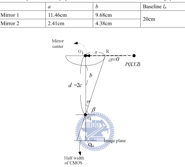
3.2.2 Details of design
In this section, we introduce the design procedure of the proposed two-mirror omni-camera in detail. An illustration of its structure is shown in Figure 2.2. The upper mirror is bigger, named Mirror 1, and the lower is smaller, named Mirror 2. They are both made to be of the hyperbolic shape. To construct the desired two-mirror omni-camera, we took two major steps as described in the following.
Step 1: Decision of the size and the position of the mirrors.
To construct the desired two-mirror omni-camera, the first step is to decide the light injection and reflection positions on the two mirrors in the imaging process. An assumption is made in advance, that is, the radius which is calculated as the distance from "the spot where the light rays are reflected from the Mirror 2" to Oci is half of the
radius which is calculated as the distance from "the spot where the light rays are reflected from the Mirror 1" to Oci.
Based onthe assumption mentioned above, a simulated omni-image is shown in Figure 3.5, where the red part is the region which is reflected by Mirror 2, and the blue part is the region which is reflected by Mirror 1. The radius of the blue region is two times to the radius of the red region.
Before deriving the formulas, we define some terms or notations appearing in Figure 3.6 which is simplified from Figure 2.2 as follows:
(1) x1 is the radius of Mirror 1;
(2) x2 is the radius of Mirror 2;
(3) d1 and d2 are the distance from Mirror 1 to the lens center, Oc and the distance
(4) f is the focal length of the perspective camera; (5) w is the width of the CMOS sensor;
(6) b1, c1 are the parameters of Mirror 1; and
(7) b2, c2 are the parameters of Mirror 2.
Figure 3.5 The desired omni-image.
In Figure 3.6, the blue lines are drawn to represent the light rays which go into the center of Mirror 1 with an incidence angle of 0o and are reflected onto the image plane (the CMOS sensor). The red lines are similarly interpreted which go into the center of Mirror 2. Then, focusing on the marked area in Figure 3.6, we get two pairs of similar triangles, (△AO1Oc, △DOciOc) and (△BO2Oc, △COciOc). By the property of similar
triangles, we can describe the relationship between them by the following equations:
ci 1 1 DO x d f , (3.4) ci 2 2 CO x d f (3.5)
Figure 3.6 A simplified modal from Figure 3.4.
Step 2: Calculation of the parameters of the mirrors.
The second step is to calculate the parameters of the hyperbolic shape of the mirrors. As shown in Figure 3.4, the relation between the CCS and the ICS of an omni-camera system, as derived by Wu and Tsai [7], may be described by
2 2 2 2 ( ) sin 2 tan ( ) cos b c bc b c , (3.6) 2 2 cos f r r , (3.7) 2 2 sin f r f , (3.8)
where r u2 v2 in the ICS, α is the elevation angle of the mirror, and β is the depression angle of Oc.
Let the omni-camera have the largest FOV, and the incidence angle be 0o, which specifying a light ray going from a point P(X, Y, Z) into the mirror center and is reflected to the image plane. As illustrated in Figure 3.7 which is a simplified version of Figure 3.4, from △O1ROc we can obtain the following equations:
d x tan , (3.9) 2 , (3.10)
where d is the distance from the mirror center to the lens center, and x is the radius length of the mirrors. In addition, we can obtain the following equation:
2 2 2 2 ( ) sin 2 tan 0 ( ) cos b c bc b c (3.11)
based on Equation (3.6) with 0.
Equation (3.11) may be transformed, by multiplying the denominator by (b2-c2)cosθ, to be:
(b2+c2)sinθ-2bc=0, (3.12)
or equivalently, to be
b2sinθ-2cb+c2sinθ=0 (3.13)
2 2 2 2 2 (2 ) 4 sin , 2 sin c c c b or equivalently, 2 2 2 2 (2 ) [1 sin ] 2sin c c b . (3.14)
Combining Equation (3.10) and Equation (3.14), we get
2 2 2 2 (2 ) [1 sin ( )] 2 2 sin ( ) 2 c c b (3.15)
which can be simplified in the following way:
2 2 2 2 2 (2 ) [1 cos ] , 2 cos 2 (2 ) sin , 2 cos 2 (2 ) sin , 2 cos c c b c c c c (1 sin ) cos c . (3.16)
Because d is the distance from a focus pointof the hyperbolic shape (the mirror center) to the other focus point Oc (the lens center) as shown in Figure 3.6, we can
obtain the parameter cof the mirror by
c=0.5 × d. (3.17)
1 1 0.5 (1 sin[tan ( )]) . cos[tan ( )] x d d b x d (3.18)
Now we can use the general analytic equations, Equations (3.17) and (3.18), to compute the parameters of the mirrors as long as we have the values of x and d.
To calculate the parameters of Mirror 2, we have to make a second assumption, that is, the radius x2 is a pre-selected value. Accordingly, we can obtain the distance d2
in Equations (3.5), and then use Equations (3.17) and (3.18) to calculate the parameters b2 and c2. And the parameter a2 may be computed by Equation (3.2).
Finally, we want to get the parameters of Mirror 1. It is mentioned in [12] that a longer baseline (shown as O O1 2 in Figure 3.6, whose width is equal to d1 d2) of the
two mirrors will yield a larger disparity (the difference between the elevateon angles) of the two mirrors in the image. If the baseline is too smaller, the range data will not be accurate. Therefore, we assume the baseline to be of an appropriate length, denoted say as lb as shown in Table 3.1, so that we can get d1 = d2 + lb and so the value of x1 by
Equation (3.4). Then, we can get the parameters b1 and c1 of Mirror 1 by using the
general equations of (3.17) and (3.18), and the parameter a1 may be computed
accordingly by Equation (3.2).
The calculated parameters of the proposed two-mirror omni-camera are shown in Table 3.1 and some simulation images of the camera are shown in Figure 3.8. We use Equation (3.3) to create the simulation images with a focal length of 6 mm and the parameter values listed in Table 3.1. As illustrated in Figure 3.8, the top-left image is the perspective image; the top-right image and the bottom-right image are the simulation images taken by Mirror 1 and Mirror 2, respectively; and the bottom-left image is the simulation image which is composed of the top-right and the bottom-right
one.
Table 3.1 The parameters of the proposed two-mirror omni-camera obtained from the design process.
a b Baseline lb
Mirror 1 11.46cm 9.68cm
Mirror 2 2.41cm 4.38cm 20cm
3.2.3 3D data acquisition
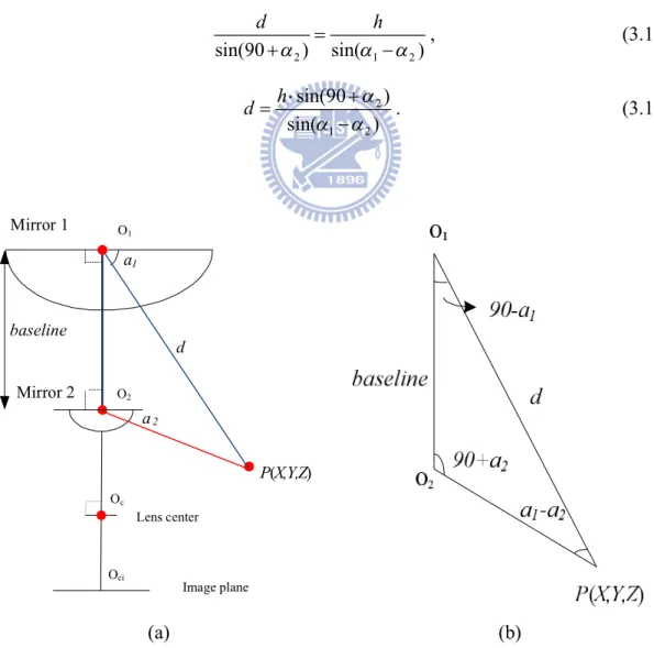
In this section, we will introduce the principle of the computation of the 3D range data and the derivation of it in the proposed system. In Figure 3.9(a), the point P in the CCS goes through each center of the two mirrors, and α1 and α2 are the
elevation angles in each mirror, respectively. A triangle △O1O2P formed by two light
rays (the blue line and the red line) is shown in Figure 3.9(b). The distance d is between the point P and O1, and the baseline length of the two mirrors is the distance
h between O1 and O2. We can derive the following equations by the law of sines based
on the geometry shown in Figure 3.9(b):
2 1 2 sin(90 ) sin( ) d h , (3.12) 2 1 2 sin(90 ) sin( ) h d . (3.13) a1 d baseline Mirror 2 Mirror 1 P(X,Y,Z) a2 O1 O2 Oc Image plane Oci Lens center (a) (b)
Figure 3.9 Computation of 3D range data using the two-mirror omni-camera. (a) The ray tracing of a point P in the imaging device. (b) A triangle in detail (part of (a)).
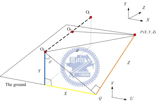
Based on Figure 3.9, a front-facing placement of the two-mirror omni-camera on the autonomous vehicle is shown in Figure 3.10 with the CCS specified by the axes of (X, Y, Z) and the ICS specified by the axes of (U, V). The optical axis OcO1 is
parallel to the ground, where Oc is the camera center, O2 is the center of Mirror 2,
and O1 is the center of Mirror 1.
From Figure 3.10, the azimuth θ in the ICS can be computed by use of the image coordinates (u, v) of P in the following:
2 2 2 2 ; cos sin v u v v u u . (3.14)
After we obtain d by Equation (3.13), by involved geometry we can compute the values of (X, Y, Z) by the following equations:
X = d × cosα1 × sinθ,
Y = d × cosα1 × cosθ,
Z = d × sinα1. (3.15)
In the proposed system, the optical axis instead is not arranged to be parallel to the ground in order to expand the overlapping area of the both mirrors, and the reason is mentioned in detail in Chapter 2. Figure 3.11 is a side view of Figure 3.10 and is shown to illustrate the slanted-up placement of the two-mirror omni-camerain the proposed system. Specifically, let the optical axis of the camera of the proposed camera system be elevated by the angle of γ, and the position of P(X, Y, Z) be translated to P′(X′, Y′, Z′) in the new coordinate system. Then, according to the trigonometry principle, we can use a rotation matrix R to represent the relationship between P and P′ as follows for computing the new coordinates (X′, Y′, Z′):
) cos( ) sin( ) sin( ) cos( R . (3.16)
As a summary, we have introduced in this chapter the design principle of the proposed two-mirror omni-camera and derived some equations we used for the related imaging processing and 3D data acquisition processes. We will describe the proposed method to calibrate the designed two-mirror omni-camera in the next chapter.
O1 O2 Oc P (X , Y , Z) d Y Z X Q The ground X Y Z U V
Figure 3.10 The frontal placement of the two-mirror omni-camera.
Chapter 4
Calibrations of Vehicle Odometer
and Proposed Two-mirror
Omni-camera
4.1 Introduction
In this chapter, we describe how we calibrate the two major devices in the proposed system, namely, (1) the odometer which is used to record the position and the direction of the autonomous vehicle, and (2) the proposed two-mirror omni-camera which is used to “see” the situation in environments. We will show the calibration method to correct the vehicle odometer in Section 4.2 and the calibration of the proposed two-mirror omni-camera in Section 4.3.
4.2 Calibration of Vehicle Odometer
4.2.1 Idea of proposed odometer calibration method
Before using any machine, a calibration process for it is usually necessary. When the autonomous vehicle is moving, the information about its direction and position is provided by the odometer in the vehicle. In a short experiment which we conducted for calibration of the odometer, we controlled the autonomous vehicle manually, and recorded the real position reached by the vehicle as well as the odometer readings at the reached spot. We found that the odometer values are not the same as the real position, and that the mechanical error increases as the vehicle’s move distance increases.
In this study, we have designed a careful experiment to test the mechanical error. We used the tiles on the floor in our laboratory to assist locating the autonomous vehicle in the experiment. Figure 4.1 shows the floor of the laboratory and each tile on it has a square shape with size 30.5cm×30.5cm. The equipments we used in this experiment are sticky tapes, a measuring tape, two laser levelers, and the autonomous vehicle.
The steps of the experiment are described as follows and shown in Figure 4.2.
1. Paste sticky tapes forming a shape of L on the floor by extending the straight lines between several tiles.
2. Use the laser levelers to adjust the heading of the autonomous vehicle to be parallel to a line of the L-shape and let the vehicle lie on the L-shape.
3. Command the vehicle to move forward on the L-shape with a distance of N tiles, where N = 3, 6, 9, 12.
4. Stop the vehicle after it moves for a distance of N tiles.
We found the position that the vehicle arrived at is no more on the L-shape and that the moving path is deviated to the left. We then measured the amount of deviation, fit the resulting deviations of several vehicle movements as a curve of the second order, and use the curve to calibrate the odometer reading of the vehicle in subsequent navigations. More details will be described subsequently. The curve fitting technique we use is described in the next section.

![Figure 3.2 The possible shapes of reflective mirrors are used in omni-cameras [7].](https://thumb-ap.123doks.com/thumbv2/9libinfo/8255614.171878/39.892.150.749.116.292/figure-possible-shapes-reflective-mirrors-used-omni-cameras.webp)