太平洋週邊國家CO2氣體排放減量的影子價格

行政院國家科學委員會專題研究計畫 成果報告

太平洋週邊國家 CO2 氣體排放減量的影子價格

計畫類別： 個別型計畫 計畫編號： NSC93-2415-H-009-001- 執行期間： 93 年 08 月 01 日至 94 年 07 月 31 日 執行單位： 國立交通大學經營管理研究所 計畫主持人： 胡均立 計畫參與人員： 林育萍 報告類型： 精簡報告 處理方式： 本計畫可公開查詢

中 華 民 國 94 年 10 月 27 日

太平洋週邊國家CO

₂

氣體排放減量的影子價格

The Shadow Prices of CO

2

Emission Abatement for Pacific-Rim Countries

計畫編號：NSC93－2415－H－009－001

執行期限：93 年 8 月 1 日至 94 年 7 月 31 日

主持人：胡均立 國立交通大學經營管理研究所

研究助理：林育萍

電子信箱(E-mail)位址：jinlihu@mail.nctu.edu.tw

一、中文摘要

關鍵詞：資料包絡分析法、非意欲產出、CO2減量、影子價格、投入距離函數 影子價格係在缺乏市場交易價格下，用來計算消費好財（good）的單位價值，或 拋棄壞財（bad）所必須之單位成本。目前環境經濟學文獻中，常見利用資料包絡分析 法（DEA）來估計多產出-多投入之決策單位（DMU）處理一單位壞財（例如：污染） 所必須支付的影子價格。 既存文獻多應用此方法於估計個別廠商或地區污染減量的影子價格。資料包絡分 析法也可以用來估計一個國家的生產力與效率，過去的生產力與效率文獻鮮少將環保因 素直接當成一個國家的投入或產出。然而，忽略環境因素，可能會嚴重高估或低估一個 經濟體或地區的生產力與效率。本研究利用Färe et al. (1993) 的一種資料包絡分析法（投 入距離函數），來估計太平洋週邊地區國家各年度的人均CO2排放減量的影子價格。 本研究採產出距離函數，將應用分析對象提高到國家層次，來估計亞太地區經濟 體CO2減量的影子價格，而資料包絡分析法會同時產生各國的技術效率值。本研究設定

每個經濟體有兩種產出：人均GDP（1996 年國際價格美元）及人均CO2（立方噸碳）。

其中GDP為意欲產出，CO2為非意欲產出。每個經濟體有兩種投入：資本形成（1996 年

國際價格美元）與勞動（人均勞動投入比率）。根據資料蒐集及研究對象區域，選擇了

19 個太平洋週邊經濟體，作為研究對象：Australia, Canada, Chile, China, Columbia, Hong

Kong, Indonesia, Japan, Korea, Malaysia, Mexico, New Zealand, Papua New Guinea, Peru,

the Philippines, Singapore, Taiwan, Thailand, and the United States。本計畫所選取的樣本期 間為 1987 至 1996 年，主要資料來源為Penn World Table Version 6.1 及Carbon Dioxide

Information Analysis Center。

我們首先利用線性規劃方法，求解超越對數投入距離函數的的各項參數值。接著 利用這些參數值及實際觀察值，產生各經濟體的效率值、及人均CO2排放減量的影子價 格（以減少的人均GDP計算）。主要發現如下：(1) 在 1987-1996 的研究期間裡，各經濟 體CO2排放減量的影子價格皆呈現逐年遞增的趨勢。(2) 一般而言，已開發經濟體每人 減量一立方噸碳排放的人均代價，遠高於開發中經濟體。(3) 雖然美國的平均效率值高 居第 2 名，在研究期間內它的CO2減量影子價格卻總是最高的。(4) 加拿大及澳大利亞 的CO2減量影子價格也很高。(5) 雖然中國大陸的平均效率值最低，在研究期間內它的 CO2減量影子價格卻很低。(6) 台灣的CO2減量影子價格在研究對象中居中。 詳細的研究成果，煩請參閱所附的英文摘要及全文部份。

二、英文摘要與英文全文

The Shadow Prices of CO

₂

Emission Abatement for

Pacific-Rim Countries

Jin-Li Hu

*

Abstract. We examine the overall macroeconomic performance and compute shadow prices of their per capita CO2 reduction of nineteen APEC economies, including Australia, Canada, Chile, China, Columbia, Hong

Kong, Indonesia, Japan, Korea, Malaysia, Mexico, New Zealand, Papua New Guinea, Peru, the Philippines, Singapore, Taiwan, Thailand, and the United States during the 1987-1996 period. We first use the linear programming approach to solve for parameters of the translog input distance function. There are two inputs (per capita capital formation and per capita labor), one desirable output (per capita GDP), and one undesirable output (per capita CO2 emission). All variables in monetary units are in USD in 1996 international prices.

We then generate the efficiency scores and shadow prices (in per capita GDP) with data and parameters obtained from linear programming. Our major findings are as follows: (1) Shadow prices of CO2 reduction were

strictly increasing for every economy during the 1987-1996 research period. (2) Generally speaking, it is much costlier for a developed economy to reduce one metric ton of carbon per capita than a developing economy. (3) Although the U.S. had the second highest average macroeconomic efficiency among these APEC economies, its shadow prices of CO2 reduction were always the highest during the research period. (4) It is also very costly

for Canada and Australia to reduce CO2 emission. (5) Although China had the lowest macroeconomic

efficiency scores, its per capita shadow prices to reduce per capita CO2 emissions were still very low. (6)

Taiwan’s shadow prices to reduce CO2 emission were medium among APEC economies.

Keywords: Undesirable outputs,CO2 reduction, input distance function, shadow prices,

technical efficiencies.

JEL Classification: C61, O13, Q43

*

This is a preliminary draft. Comments are very welcome. Correspondence: Jin-Li Hu, Institute of Business and Management, National Chiao Tung University, 4F, 114, Sec. 1, Chung-Hsiao W. Rd., Taipei City 100, Taiwan. E-mail: jinlihu@yahoo.com. URL: http://www.geocities.com/jinlihu.

1. Introduction

The Kyoto Protocol (1997) set a specific timetable for each country under the Convention

on Climate Change. The specific country target for each country is to reduce the

greenhouse gases emission from the year of 2008 to 2012 to less than the level of the year of

1990. The international and legally binding Kyoto Protocol has entered into force on

February 16, 2005. Earlier on December 12th, 2003, the Chicago Climate exchange has

started the emission trading of CFI (Carbon Financial Instrument). The relevant welfare

changes after signing the Kyoto Protocol are major concerns for the individual state’s

decision in accession to the Kyoto Protocol. The US has indicated its intention not to ratify

the Kyoto Protocol while Russia has ratified the Kyoto Protocol in October 2004.

In order to achieve the country target, the Kyoto Protocol establishes three innovative

mechanisms. Aside from countries, businesses, environmental NGOs and other legal

entities may participate in the mechanisms: (1). Joint Implementation: an Annex I Party of

Kyoto Protocol may implement a project that reduces emissions (e.g., an energy efficiency

scheme) or increases removals by sinks (e.g., a reforestation project) in the territory of

another Annex I Party, and count the resulting emission reduction units against its own target.

(2). Clean Development Mechanism: Annex I Parties may implement projects in

non-Annex I Parties that reduce emissions and use the resulting certified emission reductions

to help meet their own targets. The clean development mechanism also aims to help

non-Annex I Parties achieve sustainable development and contribute to the ultimate objective

of the Convention. (3). Emissions Trading: an Annex I Party may transfer some of the

emissions under its assigned amount to another Annex I Party that finds it relatively more

difficult to meet its emissions target.

according to differing commitments. Annex I Parties include the industrialized countries

that were members of the OECD in 1992, plus countries with economies in transition (EIT

Parties), including the Russian Federation, the Baltic States, and several Central and Eastern

European States. Annex II Parties consist of the OECD members of Annex I, but not the

EIT Parties. Non- Annex I Parties are mostly developing countries.

There are some famous cases for important APEC economies to reject the Kyoto

Protocol: Australia, Canada, and the United States (the New Scientist website, 2005;

Vedantam, 2005). These economies are developed economies while they still refuse to

follow the goals of the Kyoto Protocol. However, most the developing APEC economies

signed the Kyoto Protocol.

An economy’s macroeconomic policies generally have two objectives: creation of

wealth and good living condition for its citizens. Gross domestic product (GDP) is

commonly used in assessing an economy’s wealth. However, it does not constitute a

measure of welfare say for example without dealing with environmental issues adequately.

There is necessity to calculate environmental degradation as a correction factor into our

regular definition of economic growth (van Dieren, 1995). For the last three decades, Asia

has emerged as one of the most important economic regions of the world.

Since the 1960s, the economy of China, Hong Kong, Indonesia, South Korea, Malaysia,

Singapore, Taiwan and Thailand together have grown more than twice as fast as the rest of

Asia (Angel and Cylke, 2002). As Asia’s economic activities began to shift toward industry

and manufacturing, there has been a dramatic increase in pollution in the region (World Bank,

1998). For instance, fast-developing Asia is now one of the major contributors to the global

increase in carbon emissions (Hoffert et al., 1998; Siddiqi, 2000). In fact, the highest

percentage rises came from the Asia-Pacific region, including India, China and the newly

generally acknowledged as a cause of global warming, the United Nation has been trying to

negotiate a global agreement to tackle carbon dioxide emissions. The Kyoto protocol in

1997 was an international milestone of this effort.

The conflict between economic priorities and environmental interests, for a long time, is

at the national level since 1960s. However, as Mol (2003) states, there is an increasing clash

of economic and environmental institutions, regimes and arrangements at international level

in recent decades. Studies for economic versus environmental issues is now in a

transnational arena. For OECD members, the objective to pursue a balance between

pro-development and pro-environment has received considerable attention. Lovell et al.

(1995) study the macroeconomic performance of 19 OECD countries by extended data

envelopment analysis (DEA) approach, namely Global Efficiency Measure (GEM) for single

period analysis. Japan is the only Asian country included in their sample. The study takes

four services, real GDP per capita, a low rate of inflation, a low rate of unemployment, and a

favorable trade balance as four outputs. When two environmental disamenities (carbon and

nitrogen emissions) are included into the service list, the rankings change, while the relative

scores of the European countries decline. According to the experience of the OECD

countries, environmental indicators do seem to have crucial effects on a nation’s relative

performance.

The aim of this paper is to measure the macroeconomic performance of APEC

economies by moderating unwanted externalities of economic growth using panel data over

the period 1987-1996. In this study, performance is defined in light of an economy’s ability

to provide its citizens with both more wealth and less polluted environments. We will

examine the overall macroeconomic performance and compute shadow prices of their per

Columbia, Hong Kong, Indonesia, Japan, Korea, Malaysia, Mexico, New Zealand, Papua

New Guinea, Peru, the Philippines, Singapore, Taiwan, Thailand, and the United States.

Based on the economic theory of production, inputs (such as capital and labor) are

transformed into outputs (such as gross domestic product, GDP) in the production process.

The environmental disamenities are added and the analysis as undesirable outputs. The CO2

emissions are included as undesirable outputs.

There are three more sections besides this introductory section. The next section

provides an introduction of the distance function and linear programming model. Section 3

describes data selection. Section 4 presents the empirical results.

2. The Parametric Linear Programming Method

An economy employs N inputs denoted by a vector X =

(

x₁,x₂,",x_N

)

to produce M outputs denoted by a vector Y =

(

y₁,y₂,",y_M

)

. According to Shephard (1970), the input distance function can be defined as follows:

(

Y,X

)

sup

{

:

(

X

)

L(Y)

}

D_i =

λ

λ

∈

λ (1)

where is the input sets of production technology, describing the sets of input vectors

that can produce the output vector, Y. That is, )

(Y

L

L(Y) = {X : X can produce Y}. (2)

The input distance function gives the maximum amount by which an input vector can be

deflated and still remain producible with a given output vector. It is non-decreasing, linearly

undesirable outputs (Hailu and Veeman, 2000; Kumbhakar and Lovell, 2000). We assume

that undesirable outputs satisfy the property of weak disposability. Under weak

disposability, undesirable outputs are not to be freely disposable.

Note that D_i(Y,X)≥1 if X belongs to the input set of Y

(

X∈L(Y)

)

and that if X belongs to the frontier of the input set (the isoquant of Y). Furthermore,

the Farrell input-oriented measure of technical efficiency coincides with the reciprocal of the

input distance function (Färe and Primont 1995, Kumbhakar and Lovell 2000). 1

) , (Y X = D_i

Suppose that L(Y) is convex. Then the input distance function and the cost

function are dual (Färe and Primont, 1995):

) , (Y X D_i ) , (Y W C

{

: ( , ) 1

}

inf ) , (Y W = WX D Y X ≥ C _i X (3)

{

:

(

,

)

1

}

inf

)

,

(

Y

X

=

WX

C

Y

W

≥

D

W i (4)

where denotes the input price vector and is the inner product of

the input prices and quantity vectors. Equation (3) states that the cost function can be

derived from the input distance function by minimization over inputs X, while equation (4)

represents that the input distance is obtained from minimization with respect to input prices

W.

(

w w w_N

W = ₁, ₂,",

)

WX

Suppose that both and are differentiable. The cost function can

be represented by forming Lagrange problem: ) , (Y X D_i C(Y,W)

(

,

)

(1 ( , )) minC Y W WX D_i Y X X − + = λ , (5)

where λ is the Lagrangian multiplier. Applying the envelope theorem, we have the output shadow price vector R* =

(

r₁*,r₂*,",r_M*

)

by differentiating the cost function with respect to outputs,

(

,

)

(

,

)

( , )

* _{C Y W Y W D Y X}

R =∇_Y =−λ ∇_{Y i} . (6)

equation (6), is equal to the value of the optimized cost function (Färe and Primont

1995). The shadow price of a given output is the increasing cost resulted from the

production of additional unit of that output. The shadow price for the undesirable output

can be interpreted as the measure of the marginal cost of reducing it to the economy. Since

the input prices W are unable to obtain directly, the cost function cannot be

accurately estimated. Equation (6) indicates that the ratio of the shadow prices of output j

and output k is ) , (Y W C ) , (Y W C

(

)

(

)

k i j i k j y X Y D y X Y D r r ∂ ∂ ∂ ∂ = , , * * . (7)

Equation (7) indicates how many units of output k (say CO2 emission) the economy is willing

to give up to reduce one more unit of output j (say NPL). Assume that the market price of

output k equals its shadow price . We then could calculate the shadow price of output j

by the following formula (Färe et al. 1993, Hailu and Veeman 2000): * k r * j r

(

)

(

)

_k i j i k j y X Y D y X Y D r r ∂ ∂ ∂ ∂ = , , * * ₍₈₎

This study will employ equation (8) to calculate the shadow price of NPL. Because the cost

minimization implies cost efficient, the shadow price discussed above should be computed at

the production frontier. In other words, the shadow price formula of equation (8) should be

evaluated at the technically efficient projection of the associated input vectors (Hailu and

Veeman 2000).

In order to apply the shadow price formula, we have to parameterize and calculate the

parameters of the input distance function. An appropriate functional form to the input

distance function would ideally be flexible, easy to calculate, and permit the imposition of

homogeneity. The flexible translog functional form provides a second-order Taylor

used by many researchers (Färe et al. 1993, Lovell et al. 1994, Grosskopf et al. 1996, Hailu

and Veeman 2000).1 Furthermore, this does not impose the strong disposability of outputs.

The translog distance function with M outputs and N inputs is specified as:

m M m m N n n n i Y X x y D ( , ) ln ln ln 1 1 0 + ∑ + ∑ = = =

β

α

α

(

ln

)(

ln

)

2

1

1 1 n N n n N n nn

x

x

_′ = ′= ′

∑ ∑

+

β

)

ln

)(

ln

(

2

1

1 1 m M m m M m mm

y

y

_′ = ′= ′

∑ ∑

+

α

(

ln

)(

ln

)

1 1 m N n n M m nm

y

x

∑ ∑

+

= =

γ

. (9)

This research employs the linear programming suggested by Aigner and Chu (1968) to

estimate unknown parameters. This method relies on the minimization of the sum of

deviations of the values of the logarithmic values of the input distance from the frontier. In

other words, we try to estimate the parameters of a deterministic translog input distance

function by solving the following problem:

Min [ln ( , ) ln1] (10) 1 ∑ − = K k k k i Y X D subject to (i) lnD_i(Yk,Xk)≥0, k =1,...,K, (ii) n N k K x X Y D k n k k i _{0, 1, , , 1, ,} ln ) , ( ln " " = = ≥ ∂ ∂ (iii) m h k K y X Y D k m k k i _{0, 1, , , 1, ,} ln ) , ( ln " " = = ≤ ∂ ∂ (iv) m h M k K y X Y D k m k k i _{0, 1, , , 1, ,} ln ) , ( ln " " = + = ≥ ∂ ∂ (v) 1, 1 =

∑

= N n n β n=1 ", ,N 1

The Cobb-Douglas functional form, which is one of the most popular functional forms in production analysis, only satisfies the latter two points, because of its restrictive elasticity of substitution and scale property. Moreover, it is not an appropriate model of a firm in a competitive industry since it is not concave in output dimensions (Klein 1953).

∑ = = ∑ = = ′ ′ N n nm N n 1nn 1 0 γ β m=1,",M, n=1,",N (vi) α_mm′ =α_m′m, m=1,,",M, m′=1,",M N n N n n n n n ′ =β ′ , =1,", , ′=1,", β

where indexes individual banks; has the explicit functional

form described in equation (9), the first h outputs are desirable; and the other (K − h) outputs are undesirable.

K

k =1 ", , lnD_i(Yk,Xk)

The first constraint indicates that all banks are within the technology frontier.

Constraint (ii) is the condition that the input distance function is non-decreasing in inputs.

There exists a fundamental asymmetry between desirable and undesirable outputs that

desirable outputs are freely disposable, while reducing undesirable outputs are costly.

Constraints (iii) and (iv) are hence required to guarantee that the input distance function is

non-increasing and non-decreasing function of, respectively, desirable and undesirable

outputs. The last two constraints guarantee the linear homogeneity in inputs for the input

distance function (v) and the parameters symmetry condition for the translog functional form

(vi).

3. Data Sources

The nineteen selected economies are all APEC members: Australia (AUS), Canada

(CAN), Chile (CHL), China (CHN), Columbia (COL), Hong Kong (HKG), Indonesia (IDN),

Japan (JPN), Korea (KOR), Malaysia (MLS), Mexico (MEX), New Zealand (NZL), Papua

New Guinea (PNG), Peru (PER), the Philippines (PHL), Singapore (SNG), Taiwan (TWN),

Thailand (THA), and the United States (USA) during the 1987-1996 period. We then

construct an APEC efficiency frontier for these ten years based on the macroeconomic data of

efficiency frontier and associative indices such as efficiency scores and shadow prices of CO2

reduction can be hence found.

There are two inputs and two outputs. We take capital formation and labor force as two

inputs and GDP per capita as a desirable output for a specific economy. These data are from

Penn World Table Version 6.1 provided by Center for International Comparisons at the

University of Pennsylvania (CICUP, 2002). The value of monetary inputs and outputs such

as GDP per capita and capital formation are counted by USD in 1996 international prices.

Although capital formation and labor force are not directly available from the data set, simple

calculation can be applied: The capital formation is retrieved from the product of real GDP

per capita and investment share of real GDP per capita (USD in 1996 international prices),

while the labor force is calculated by dividing real GDP per capita with real GDP per worker.

The data of per capita CO2 emissions (metric tons of carbon) is from Carbon Dioxide

Information Analysis Center (Marland et al., 2003). The data after 1996 are not included

due to the lack of data for certain economies.

Macroeconomic performance is evaluated in terms of the ability of an economy to

maximize the desirable output GDP while minimizing the CO2 emissions. Summary

statistics of these inputs and outputs are shown in Table 1.

[Insert Table 1 about here]

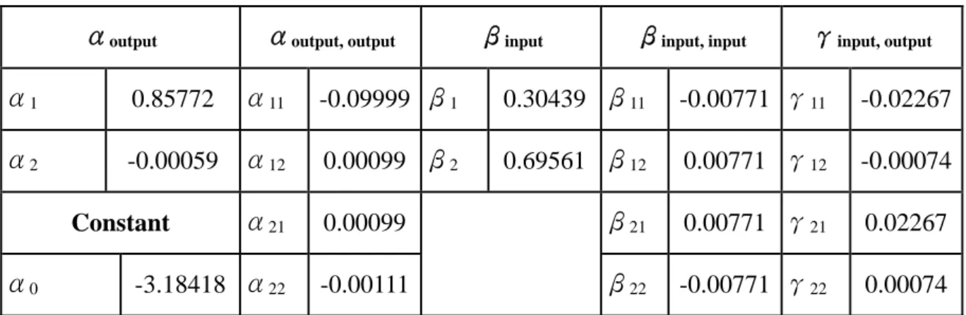
This study employs the mathematical programming software LINGO 6.0 to compute the

parameters of the translog input distance function. Table 2 shows the values of estimated

parameters. These parameter estimates were used to calculate the technical efficiencies, the

reciprocal of the input distance function, and the shadow prices of CO2 reduction (Equation

per capita) is exactly one USD. I then use the statistical software TSP 4.5 to generate

efficiency scores and shadow prices.

[Insert Table 2 about here]

4. Empirical

Results

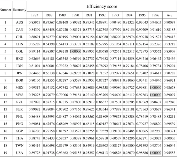
The macroeconomic efficiency scores with CO2 emissions considered are listed in Table

3. These rankings are stable during the 1987-1996 research period. The APEC economies

ranked from the highest to the lowest average efficiency scores are: Mexico (0.98678), the

United States (0.95553), Australia (0.90097), Chile (0.89413), Malaysia (0.89097), Canada

(0.88183), New Zealand (0.87940), Korea (0.86921), Peru (0.86341), Taiwan (0.86044),

Columbia (0.85909), the Philippines (0.82211), Singapore (0.80371), Hong Kong (0.78436),

Indonesia (0.79294), Japan (0.70282), Papua New Guinea (0.69539), Thailand (0.60005), and

China (0.53212).

[Insert Table 3 about here]

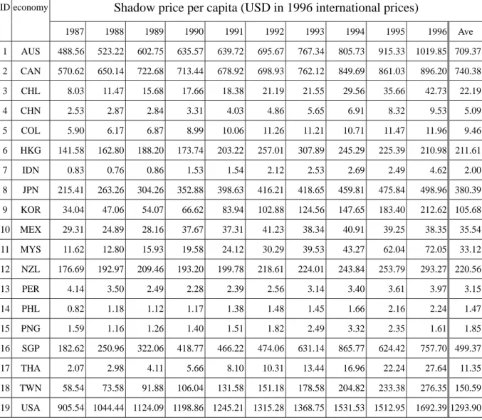
The shadow prices (per capita USD in 1996 international prices) of per capita CO2

reduction (metric tons of carbon) considered are listed in Table 4. Rankings in shadow

prices are also stable during the 1987-1996 research period. The APEC economies ranked

from the lowest to the highest average shadow prices are: Peru ($1.47), the Philippines

($1.85), Indonesia ($2.00), Papua New Guinea ($3.15), China ($5.09), Columbia ($9.46),

Thailand ($11.35), Chile ($22.19), Mexico ($33.12), Malaysia ($35.54), Korea ($105.68),

New Zealand ($220.56), Hong Kong ($211.61), Japan ($380.39), Singapore ($499.37),

Taiwan ($150.59), Australia ($709.37), Canada ($740.38), and the United States ($1293.90)

[Insert Table 4 about here]

Many interesting observations can be obtained from our empirical results:

(1) The shadow prices of CO2 reduction were strictly increasing for every economy during

the 1987-1996 research period. That is, it has been becoming costlier for each economy

to reduce one metric ton of carbon per capita as time goes by.

(2) Generally speaking, it is much costlier for a developed economy to reduce one metric ton

of carbon per capita than a developing economy.

(3) Although the U.S. had the second highest average macroeconomic efficiency among

these APEC economies, its shadow prices of CO2 reduction were always the highest

during the 1987-1996 research period. This can explain why the U.S. still refuses to

sign the Kyoto Protocol even until 2005.

(4) Cases similar to the U.S. also happened to Canada and Australia. It is also very costly

for Canada and Australia to reduce CO2 emission. This can explain why Australia and

Canada still reject the Kyoto Protocol even until 2005.

(5) Although China had the lowest macroeconomic efficiency scores, its per capita shadow

prices to reduce per capita CO2 emissions were still very low.

(6) Taiwan’s shadow prices to reduce CO2 emission were medium among APEC economies.

Acknowledgements

The author is indebted to Taichen Chien, Chih-Hung Kao, Yang Li, Hsin-Wei Liu, and

Shih-Fang Lo for their helpful comments and suggestions. I also thank Yu-Ping Lin for her

efficient research assistance. Financial support from Taiwan’s National Science Council

Reference

1. Angel, D. and Cylke, O. (2002). “Development: the east Asian solution,” Asian Times.

(http://www.atimes.com/atimes/Asian_Economy/DI17Dk01.html)

2. Aigner, D. J., and S. F. Chu (1968), “On estimating the industry production function,”

American Economic Review, 58, 826-839

3. Aigner, D. J., C. A. K. Lovell, and P. Schmidt (1977), “Formulation and estimation of

stochastic frontier production function models,” Journal of Econometrics, 6, 21-37

4. Banker, R. D., A. Charnes, and W. W. Cooper (1984), “Some models for estimating

technical and scale inefficiencies in data envelopment analysis,” Management Science, 30,

1078-1092

5. Battese, G. E., and T. J. Coelli (1988), “Prediction of firm-level technical efficiencies with

a generalized frontier production function and panel data,” Journal of Econometrics, 38,

387-399

6. Battese, G. E. and T. J. Coelli (1992), “Frontier production functions, technical efficiency

and panel data: with application to paddy farmers in India,” Journal of Productivity

Analysis, 3, 153-169

7. Battese, G. E. and T. J. Coelli (1995), “A model for technical inefficiency effects in a

stochastic frontier production function for panel data,” Empirical Economics, 20, 325-332

8. Center for International Comparisons at the University of Pennsylvania (CICUP) (2002).

Penn World Table 6.1. (http://pwt.econ.upenn.edu)

9. Charnes, A. S., W. W. Cooper, and E. Rhodes (1978), “Measuring the efficiency of

decision making units,” European Journal of Operational Research, 2, 429-444

10. Färe, R., S. Grosskopf, C. A. K. Lovell, and S. Yaisawarng (1993), “Derivation of shadow

Statistics, 75, 374-380

11. Färe, R. and D. Primont (1995), Multi-Output Production and Duality: Theory and

Applications, Boston: Kluwer-Academic Publishers

12. Farrell, M. J. (1957), “The measurement of productive efficiency,” Journal of the Royal

Statistical Society, 120, 253-281

13. Hailu, A., and T. S. Veeman (2000), “Environmentally sensitive productivity analysis of

the Canadian pulp and paper industry, 1959-1994: an input distance function approach,”

Journal of Environmental Economics and Management, 40, 251-274

14. Hoffert, M. I., Caldeira, K., Jain, A. K., Harvey, L. D. D., Potter, S. D., Schlesinger, M. E.,

Schneider, S. H., Watts, R. G., Wigley, T. M. L. and Wuebbles, D. J. (1998), “Energy

implications of future stabilization of atmospheric CO2 content,” Nature, 295, 881-884

15. Kopp, R. J. and W. E. Diewert (1982), “The decomposition of frontier cost function

deviations into measures of technical and allocative efficiency,” Journal of Econometrics,

19, 319-331.

16. Kumbhakar, S. C. and C. A. K. Lovell (2000). Stochastic Frontier Analysis, New York:

Cambridge University Press

17. Lovell, C. A. K., Pastor, J. T. and Turner, J. A. (1995), “Measuring macroeconomic

performance in the OECD: a comparison of European and non-European countries,”

European Journal of Operational Research, 87, 507-518

18. Marland, G., T. A. Boden, and R. J. Andres (2003), “Global, regional, and national fossil

fuel CO2 emissions,” Carbon Dioxide Information Analysis Center (CDIAC).

(http://cdiac.ornl.gov)

19. Masood, E. (1997), “Asian economies lead increase in carbon dioxide emissions,” Nature,

(http://www.nature.com/cgi-taf/DynaPage.taf?file=/nature/journal/v388/n6639/full/38821

3a0_r.html)

regimes,” International Journal of Sustainable Development and World Ecology, 10,

303-318

21. New Scientist (2005), website: http://www.newscientist.com

22. Pitt, M. M. and L. F. Lee (1981), “The measurement and sources of technical inefficiency

in the Indonesian weaving industry,” Journal of Development Economics, 9, 43-64

23. Siddiqi, T. A. (2000). “The Asian financial crisis – is it good for the global

environment?,” Global Environmental Change, 10, 1-7

24. Schmidt, P. and C. A. K. Lovell (1979), “Estimating technical and allocative inefficiency

relative to stochastic production and cost frontiers,” Journal of Econometrics, 13, 83-100

25. Schmidt, P. and R. Sickles (1984), “Production frontiers and panel data,” Journal of

Business and Economic Statistics, 2, 367-374

26. Shephard, R.W. (1970), Theory of Cost and Production Functions, Princeton: Princeton

University Press.

27. van Dieren, W. (1995). Taking Nature into Account. (New York: Copernicus)

28. Varian, H. (1984), “The nonparametric approach to production analysis,” Econometrica,

52, 579-597.

29. Vedantam, S. (2005), “Kyoto Treaty Takes Effect Today --- Impact on Global Warming

May Be Largely,” Washington Post, February 16, Page A04

Table 1. Summary Statistics of Inputs and Outputs

M e a n Standard

Deviation M i n i m u m M a x i m u m Inputs

Real capital formation per capita (USD in 1996 international prices)

2766.156 2386.044 241.090 10955.910

Labor (per capita labor input

ratio) 0.461 0.0874 0.320 0.650

Outputs

Real GDP per capita (USD in

1996 international prices) 10587.256 7667.836 1344.610 29193.910 CO2 Emission per capita (metric

tons of carbon) 1.643 1.704 0.180 6.670

Table 2. Parameter Estimates

αoutput αoutput, output βinput βinput, input γinput, output

α1 0.85772 α11 -0.09999 β1 0.30439 β11 -0.00771 γ11 -0.02267

α2 -0.00059 α12 0.00099 β2 0.69561 β12 0.00771 γ12 -0.00074

Constant α21 0.00099 β21 0.00771 γ21 0.02267

Table 3. 1987-1996 Technical Efficiencies for APEC Economies Efficiency score Number Economy 1987 1988 1989 1990 1991 1992 1993 1994 1995 1996 Ave 1 AUS 0.85953 0.87567 0.89168 0.89392 0.89547 0.89891 0.90480 0.91323 0.93043 0.94605 0.90097 2 CAN 0.84309 0.86458 0.87920 0.88374 0.87715 0.87595 0.87979 0.89156 0.90709 0.91619 0.88183 3 CHL 0.88691 0.89279 0.89195 0.89001 0.89156 0.89080 0.88290 0.88976 0.90938 0.91527 0.89413 4 CHN 0.55289 0.54398 0.54173 0.53737 0.53182 0.52795 0.51954 0.52111 0.52154 0.52326 0.53212 5 COL 0.99114 0.98507 0.99218 1.00000 0.89957 0.80688 0.72551 0.72517 0.72975 0.73562 0.85909 6 HKG 0.62666 0.64181 0.65545 0.66599 0.72737 0.79482 0.87114 0.94858 0.94716 0.96462 0.78436 7 IDN 0.81094 0.80001 0.79222 0.78697 0.78458 0.78992 0.79155 0.79184 0.78406 0.79734 0.79294 8 JPN 0.64486 0.66138 0.67646 0.69232 0.71028 0.71552 0.72077 0.72651 0.73402 0.74611 0.70282 9 KOR 0.80106 0.81555 0.82287 0.83589 0.85953 0.87327 0.88971 0.91060 0.93411 0.94946 0.86921 10 MEX 0.99317 0.97152 0.97342 0.97635 0.98089 0.98558 0.99080 0.99727 0.99881 1.00000 0.98678 11 MYS 0.79275 0.79079 0.79006 0.79181 0.92140 0.93705 0.94600 0.96119 0.97863 1.00000 0.89097 12 NZL 0.87028 0.87715 0.87875 0.87800 0.86919 0.86577 0.87501 0.88205 0.89369 0.90407 0.87940 13 PER 0.99092 0.98084 0.97802 0.97166 0.89625 0.83544 0.77878 0.73181 0.73363 0.73677 0.86341 14 PHL 0.86488 0.85993 0.84827 0.84062 0.83567 0.81809 0.79873 0.78388 0.78619 0.78483 0.82211 15 PNG 0.69081 0.67576 0.68969 0.68997 0.68115 0.69187 0.70647 0.73074 0.70927 0.68820 0.69539 16 SGP 0.76206 0.79158 0.81592 0.83525 0.82255 0.79529 0.79130 0.78485 0.80865 0.82960 0.80371 17 THA 0.58743 0.58433 0.58537 0.58388 0.58961 0.59810 0.60539 0.61296 0.62271 0.63073 0.60005 18 TWN 0.80414 0.80698 0.81979 0.83104 0.84916 0.86303 0.88127 0.89800 0.91395 0.93706 0.86044 19 USA 0.89778 0.91738 0.93662 0.95153 0.95257 0.96113 0.96876 0.98070 0.98886 1.00000 0.95553

Table 4. 1987-1996 Absolute Shadow Prices of CO2 Reduction

ID economy _{Shadow price per capita (USD in 1996 international prices)}

1987 1988 1989 1990 1991 1992 1993 1994 1995 1996 Ave 1 AUS 488.56 523.22 602.75 635.57 639.72 695.67 767.34 805.73 915.33 1019.85 709.37 2 CAN 570.62 650.14 722.68 713.44 678.92 698.93 762.12 849.69 861.03 896.20 740.38 3 CHL 8.03 11.47 15.68 17.66 18.38 21.19 21.55 29.56 35.66 42.73 22.19 4 CHN 2.53 2.87 2.84 3.31 4.03 4.86 5.65 6.91 8.32 9.53 5.09 5 COL 5.90 6.17 6.87 8.99 10.06 11.26 11.21 10.71 11.47 11.96 9.46 6 HKG 141.58 162.80 188.20 173.74 203.22 257.01 307.89 245.29 225.39 210.98 211.61 7 IDN 0.83 0.76 0.86 1.53 1.54 2.12 2.53 2.69 2.49 4.62 2.00 8 JPN 215.41 263.26 304.26 352.88 398.63 416.21 418.65 459.81 475.84 498.96 380.39 9 KOR 34.04 47.06 54.07 66.62 83.94 102.88 124.56 147.65 183.40 212.62 105.68 10 MEX 29.31 24.89 28.16 37.67 37.31 41.23 38.34 40.91 39.25 38.35 35.54 11 MYS 11.62 12.80 15.93 19.58 24.12 30.29 39.53 43.27 62.04 72.05 33.12 12 NZL 176.69 192.97 209.46 193.20 199.78 218.61 224.01 243.84 253.79 293.27 220.56 13 PER 4.14 3.50 2.49 2.28 2.39 2.56 3.14 3.40 3.61 3.97 3.15 14 PHL 0.82 1.18 1.12 1.17 1.38 1.48 1.45 1.66 2.16 2.24 1.47 15 PNG 1.59 1.16 1.26 1.40 1.51 1.82 2.49 3.32 2.35 1.61 1.85 16 SGP 182.62 250.96 322.06 418.77 466.22 474.06 631.14 865.77 624.42 757.70 499.37 17 THA 2.07 2.98 4.11 5.66 8.10 10.31 13.44 16.96 22.24 27.64 11.35 18 TWN 58.54 73.58 91.88 106.04 131.58 151.18 178.58 204.82 233.38 276.35 150.59 19 USA 905.54 1044.44 1124.09 1198.86 1245.21 1315.28 1368.75 1531.53 1512.95 1692.39 1293.90