機率式建模技術與自然語言的標記、認知和教學 (I)

行政院國家科學委員會補助專題研究計畫

□ 成 果 報 告

█期中進度報告

機率式建模技術與自然語言的標記、認知和教學

計畫類別：█ 個別型計畫 □ 整合型計畫

計畫編號： NSC-97-2221-E-004-007-MY2

執行期間： 2008 年 8 月 1 日至 2010 年 7 月 31 日

計畫主持人：劉昭麟

共同主持人：高照明、蔡介立

計畫參與人員： 賴敏華、田侃文、黃志斌、黃昭憲、莊怡軒、翁睿妤

成果報告類型(依經費核定清單規定繳交)：█精簡報告 □完整報告

本成果報告包括以下應繳交之附件：

□赴國外出差或研習心得報告一份

□赴大陸地區出差或研習心得報告一份

□出席國際學術會議心得報告及發表之論文各一份

□國際合作研究計畫國外研究報告書一份

處理方式：除產學合作研究計畫、提升產業技術及人才培育研究計畫、

列管計畫及下列情形者外，得立即公開查詢

□涉及專利或其他智慧財產權，□一年□二年後可公開查詢

執行單位：國立政治大學資訊科學系

中 華 民 國 2009 年 5 月 31 日

中文摘要

本年度的工作重點在於持續上一年度的工作內容，在機率式學生建模的工作上，持續發表

相關期刊論文。在應用自然語言處理技術於語文教學方面，也持續過去之工作，今年特別

著重於中文錯字研究與句子重組的問題上。除了這兩大類的工作之外，也與政大心理系蔡

介立教授合作研究中文母語使用者閱讀過程中的眼動路徑。整體而言，本計畫延續過去多

年的研究基礎，在過去十個月之中，接受並正式發表的論文數目有十一篇。其中期刊論文

兩篇，國際會議論文三篇，國內會議論文六篇。另有兩篇已經投稿之國際會議論文，審查

結果尚未公告。

英文摘要

In the first half of this project, we continued what we have been doing in the past few years. We

worked on the construction of student models using a probability-based approach, and continued

to publish research papers. We have also applied the techniques for natural language processing

to computer assisted language learning. In past several months, we have focused on research

issues regarding incorrect Chinese words and regarding the reconstruction of scrambled sentences.

In addition, in order to offer better assistance in learning languages, we worked with Professor

Tsai of the Department of Psychology (National Chengchi University) to study how native

speakers of Chinese move their eyes while they read Chinese. Overall, we published 11 papers in

the past 10 months. Two of them are journal articles, three are international conference papers,

and six are domestic conference papers. Two other submitted papers are still under review.

工作報告

本年度的工作內容分為三個方向：機率式學生模型的建構、應用自然語言處理技術輔助語

文教學、人類閱讀歷程之研究。在這三個方向上，本研究計畫，均已陸續發表論文，以下

以摘要方式簡報所獲致之成果與經驗，詳細之成果請讀者參考所附之論文。

機率式學生模型的建構

這一研究計畫主要是承繼過去幾年的努力，利用貝氏網路(Bayesian networks)來捕捉學生

對於綜合觀念的學習歷程，經過多年的持續努力，研究成果終於發表在國際著名的

International Journal of Artificial Intelligence in Education (IJAIED)，內容接近五十頁超過兩萬

字。另一部份未能在 IJAIED 中詳述的技術與概念，則發表於 Behaviormetrika 期刊，該期

刊是日本行動計算學會(The Behaviormetric Society of Japan)的代表期刊，期刊內容收錄於日

本 Scientific Links Japan。IJAIED 是人工智慧與教育學會(International AIED Society)的代

表期刊，該學會所主辦的 AIED 研討會、International Conference on Intelligent Tutoring

Systems 和 IEEE 的 ICALT 是電腦輔助教育這一領域中最具盛名的一些國際學術研討會。

這一項研究的工作內容是探討學生在學習多個基本觀念時，我們有沒有辦法透過測驗技

術，來探究學生如何融合個別基本觀念以習得綜合觀念。由於人們在接受測驗時，常有運

氣好答對或者運氣不好答錯的現象，因此人的外顯表現，並不一定反映其真實能力，因此

要透過學生的答題表現來探究其內心的細部狀態（即學習歷程）是一件很困難的事情。研

究結果顯示，隨著學生碰巧猜對與意外答錯的機率的變化，這一個研究問題的可達成成果

有很大的差異。除了這兩個基本變因之外，本研究也發現如何掌握學生族群的能力分佈，

也是探究學習歷程的重要因素。

本研究所應用的技術包含貝氏網路、類神經網路(artificial neural networks)、支持向量機

(support vector machines)還有一些經驗法則(heuristic rules)。技術的主軸是利用機器學習技

術來學習大量資料中的貝氏網路機率模型。

其他細節請參考論文[1,2]。

應用自然語言處理技術輔助語文教學

電腦輔助語文教學(Computer Assisted Language Learning)是國內外許多機構競相發展的技

術。世界各國的高度交流，國際化的趨勢與需求高漲，使得語文學習變得比過去更加重要。

如何能夠應用資訊通訊科技來提高學習語文的效率與成效，顯然是一件極度吸引人的研究

議題。

政大這一個研究群在過去幾年利用處理自然語言的技術，開發過不少有趣的應用環境，在

英文試題輔助出題和中文試題輔助出題方面，都有所成就，而且成果都發表在 Annual

Meeting of Association for Computational Linguistics (ACL)，ACL 的年度研討會算是計算

語言學界第一級的研討會。除了 ACL 的論文之外，部分的成果發表於今年的 IEA/AIE 年度

研討會，IEA/AIE 研討會的接受率長年都控制在 30%左右，算是應用領域中比較好的研討

會。除了國際學術會議之外，為了與國內學者交流，我們也將成果以中文撰寫，發表於計

算語言學會的 ROCLING 研討會。

在這一研究方向上，本年度的重點工作仍和去年一樣，偏重於中文錯字的研究，我們探討

了中文錯字的產生的原因，資料顯示中文錯字的產生有高達 80%的機會是因為發音的相同

或者相近，另有相當的比例是字體相近引起的。本實驗從中文改錯字的出題輔助，逐漸跨

到研究母與使用者為何寫錯字的研究，這兩份研究成果都發表於 ACL 的短文論文。工作內

容請參考論文[3,4,5,8]

在錯字研究之外，我們也研究句子重組的出題輔助系統。句子重組的試題，是把一個給定

的語句切割成一些字串，然後要求學生利用這一些打散的字串重建原始的語句。切割語句

不是困難的工作，但是要確保學生會組合成原來的語句卻不簡單。一個被打散的語句，可

可以重組為「this new car is better than that old bike」。如何輔助出題教師確保學生所重組的

答案只能是符合教學目標的那一些語句，是一件不容易達到的工作。這一部分的研究工作，

目前仍然在進行中，部分的成果已經投稿，但是評審結果仍然不知道。

長期而言，本實驗室有計畫重拾計畫主持人過去的機器翻譯研究工作，因此今年度有兩個

準備工作。一則是建置中學程度電腦輔助英漢翻譯習作的環境，一則是利用電腦軟體翻譯

數理科目的英文試題。這兩個工作的成果都已經發表於 ROCLING [9, 10]。電腦輔助英漢翻

譯習作環境的工作，主要是輔導研究生作一些基本研究工作，同時也累積實驗室一些研究

資源。技術層次雖然不能說高，但是同時具有訓練與累積研究資源的意義。電腦輔助的試

題翻譯則是面對真實的翻譯工作，我們建立了 language model 加上平行語料庫的建立，已

經具備研究翻譯系統的雛形。我們期待這一方面的努力，在未來幾年之內，能夠讓實驗室

能夠認真地進行機器翻譯的研究工作。

人類閱讀歷程之研究

在研究語文教學與電腦輔助教育的過程中，我們需要學生的學習模型。學生的模型是電腦

輔 助 測 驗 的 重 要 基 礎 ， 即 使 是

item response theory (IRT,

http://en.wikipedia.org/wiki/Item_response_theory)也可以視為是一種間接的學生模型。在 IRT

模型中，我們以統計技術建立學生表現與能力關係的模型，儲存於試題的參數之中。

在自然語言處理和語文教育裡面，我們如果能夠知道人類的閱讀與認知歷程的話，就有可

能提高計算機理解人類語文資料的技術層次。瞭解人類認知歷程，也有助於我們設計有效

率的語文學習環境。這一些都是我們走向這一研究的原因。

在過去一年之中，透過政大心理系蔡介立教授的協助，我們得以研究真人母語使用者的演

動資料，並且加以分析。研究結果顯示人與人的差異性極大，即使我們獲得珍貴的四十個

真人的演動資料，目前暫時沒有找到很肯定的模型。儘管如此，我們已經把部分成果撰寫

成一篇短文，目前處於審稿階段。

其他自然語言處理技術的應用：資訊檢索與文件分類

延續更久之前的國科會研究計畫，我們今年在 ROCLING 發表了一篇關於中文訴訟文書的

檢索系統的論文[6]。這一成果，其實是整合了過去多年研究的功能，在一整個資訊檢索的

環境之中。

學術研討會的投稿論文該由誰來擔任評審委員？這是一個很難的問題。我們可以把這一個

問題當作是一種文件分類的問題，以個別評審當作是一個類別，我們希望把所收到的稿件

分到所屬的類別。這當然是一個簡化的想像，一個研討會的評審指派有許多因素要考慮；

例如，有合作關係者不宜互審、同一評審不宜審查過多論文、同時我們也必須考慮評審的

電腦遊戲學習

這一項工作，主要是訓練一位有潛力的大學部學生，使之能夠對於機器學習技術有初步的

應用經驗。我們培養了一位大學部畢業生，習得初步的機器學習技術，應用於黑白棋(或稱

蘋果棋、Reversi、Othello)，開發出任意棋盤的 Othello 的新想法 ，並且發表一篇 TAAI 論

文[7]。該生即將加入交大吳毅成教授的研究團隊。

計畫成果自評

以政治大學資訊科學系在國內資訊領域的排名所可以收到的研究生，加上計畫主持人在研

究、教學與校外學術服務而言，計畫主持人自以為本計畫的執行是成功的。

在論文發表上，雖然我們仍有許多可以再進步的空間，但是也逐漸擠身於國際間頂尖的學

術會議與期刊論文。

在學生的培養方面，這兩年這一個實驗室為真正的頂尖大學培育了不少可用之才，就在今

年度，就有一位赴台大就讀博士班、一位赴台大就讀碩士班、一位赴交大就讀碩士班的研

究生。

本年度至今發表之論文

1. Chao-Lin Liu. Selecting Bayesian-network models based on simulated expectation,

Behaviormetrika, 36(1), 1‒25. The Behaviormetric Society of Japan, Japan, April 2009.

2. Chao-Lin Liu. A simulation-based experience in learning structures of Bayesian networks to

represent how students learn composite concepts, International Journal of Artificial

Intelligence in Education, 18(3), 237‒285. IOS Press, The Netherlands, September 2008.

3. Chao-Lin Liu, Kan-Wen Tien, Min-Hua Lai, Yi-Hsuan Chuang, Shih-Hung Wu. Phonological

and logographic influences on errors in written Chinese words, Proceedings of the Seventh

Workshop on Asian Language Resources, the Forty Seventh Annual Meeting of the

Association for Computational Linguistics (ACL’09), to appear. Singapore, 2-7 August 2009.

4. Chao-Lin Liu, Kan-Wen Tien, Min-Hua Lai, Yi-Hsuan Chuang, Shih-Hung Wu. Capturing

errors in written Chinese words, Proceedings of the Forty Seventh Annual Meeting of the

Association for Computational Linguistics (ACL’09), short papers, to appear. Singapore, 2-7

August 2009.

5. Chao-Lin Liu, Kan-Wen Tien, Yi-Hsuan Chuang, Chih-Bin Huang, Juei-Yu Weng. Two

applications of lexical information to computer-assisted item authoring for elementary

Chinese, Lecture Notes in Computer Science 5579: Proceedings of the Twenty Second

International Conference on Industrial Engineering & Other Applications of Applied

Intelligent Systems (IEA/AIE’09), 470‒480. Tainan, Taiwan, 24-27 June 2009.

6. 藍家良、賴敏華、田侃文及劉昭麟。訴訟文書檢索系統，

第十三屆人工智慧與應用研討

會論文集

(TAAI’08)，305‒312。臺灣，宜蘭，2008 年 11 月 21-22 日。(中文內容)

7. 林正宏及劉昭麟。任意棋盤的 Othello 遊戲，

第十三屆人工智慧與應用研討會論文集

(TAAI’08)，443‒449。臺灣，宜蘭，2008 年 11 月 21-22 日。(中文內容)

然語言與語音處理研討會論文集

(ROCLING XX)，108‒122。臺灣，臺北，2008 年 9

月 4-5 日。(中文內容)

9. 賴敏華及劉昭麟。電腦輔助中學程度漢英翻譯習作環境之建置，

第二十屆自然語言與語

音處理研討會論文集

(ROCLING XX)，293‒307。臺灣，臺北，2008 年 9 月 4-5 日。(中

文內容)

10. 張智傑及劉昭麟。以範例為基礎之英漢 TIMSS 試題輔助翻譯，

第二十屆自然語言與語

音處理研討會論文集

(ROCLING XX)，308‒322。臺灣，臺北，2008 年 9 月 4-5 日。(中

文內容)

11. 陳禹勳及劉昭麟。電腦輔助推薦學術會議論文評審委員之初探，

第二十屆自然語言與語

音處理研討會論文集

(ROCLING XX)，323‒337。臺灣，臺北，2008 年 9 月 4-5 日。(中

文內容)

附錄：發表論文之代表作

Chao-Lin Liu. Selecting Bayesian-network models based on

simulated expectation, Behaviormetrika, 36(1), 1‒25. The

Behaviormetric Society of Japan, Japan, April 2009.

SELECTING BAYESIAN-NETWORK MODELS BASED ON

SIMULATED EXPECTATION

Chao-Lin Liu

Identifying the best network structure from a myriad of candidates is not an easy task, and we propose a supervised learning method for this task. We test the idea with an in-stance of learning student models from students’ responses to test items, because student models are very important for intelligent tutoring systems. The training data for the classi-fiers were simulated based on the expectation about students’ item responses when stu-dents learn in different ways, and the trained classifier was used to select the model from the list of candidate models based on the observed item responses. Experimental results indicate that, even when item responses do not faithfully reflect students’ competence in the concepts, our classifiers still help us differentiate very similar models with indirect ob-servations.

1. Introduction

A simple exercise for students who are learning the modeling techniques is to find the distribu-tion over the height of a populadistribu-tion. A common strategy for solving such an exercise is to assume a Gaussian distribution and set out to find the mean and variance for the underlying distribution. The assumption is not arbitrary because many statistics for natural phenomena conform to the Gaussian distribution. The experience-based expectation helps us simplify the problem of model selection by confining the search space to the class of Gaussian distributions. We should be able to employ a similar idea to the problem of selecting Bayesian networks in the model selection task. To examine the applicability of this idea, we attempt to tackle a student modeling problem in this paper.

Furnishing appropriate educational material at appropriate timings is important in educational activities. Teachers, utilizing their professional knowledge and experience, may judge the timing, choose the material, and provide individualized guidance when they interact directly with their stu-dents. When building intelligent tutoring systems, we attempt to capture and express the profes-sional knowledge and experience in both student and teacher models so that the resulting products can assist students’ learning when teachers are not immediately available.

Building good models of teachers and students is not a simple task. It takes a lot of training for an ordinary person to become a qualified teacher, and it takes even more time and costs for a novice teacher to turn experienced. On the other hand, students vary in a wide range of ways. They differ in their competence and in their interests, for instance; and the needs for the same student may also change over time. As a result, it demands plenty of effort to build computational models of teachers and students, so different research projects focus on diverse aspects of students when they discuss student modeling.

In this paper, we discuss an application of supervised learning methods for selecting candidate Bayesian networks, and test the idea with the problems of modeling how students learn composite concepts. We assume that there are test items which are designed to test the competence in related concepts. We also assume the availability of students’ responses to these test items, and use the item responses to select the best model from the candidate models that are provided by domain experts. The domain experts do not need to provide the class tags for students’ data as in most supervised learning. Instead, the domain experts specify the structures and ranges of parameters for the candi-date models, with which we create simulated data based on the candicandi-date models, and use these

Key Words and Phrases: Student Modeling, Intelligent Tutoring, Learning Bayesian Networks, Model

Selec-tion, Computational CogniSelec-tion, Causal Modeling, Supervised Learning

* _{Department of Computer Science, National Chengchi University, Wen-Shan, Taipei 11605, Taiwan.}

E-mail: [email protected]

simulated data and their class tags to select the candidate model that fits students’ item responses. Experience shows that students’ external behaviors do not necessarily reflect their internal states. In educational assessment problems, students may fail to answer some test items correctly when they are competent in the concepts that are being tested, and, conversely, student may answer correctly just because of lucky guesses when they are not competent (e.g., VanLehn et al., 1994; Millán & Pérez-de-la-Cruz, 2002). We will refer to the former cases, slip, and the latter cases, guess, in this paper. We employ Bayesian networks (Pearl, 1988; Jensen & Nielsen, 2007) to capture this uncertain relationship between students’ competence in concepts and their responses to test items.

To acquire composite concepts, students need to combine their knowledge about two or more other concepts to form the new concept. These “other” concepts can be basic concepts or composite concepts. For instance, to add two fractions that have different denominators, we have to convert these fractions to have a common denominator and then add the numerators. To convert the original fractions to have a common denominator, students need to comprehend the concept about common multiples which is based on a more fundamental concept—the concept about multiples. Hence, the concepts about multiples, common multiples, making fractions to have a common denominator, and adding two fractions with a common denominator are needed to add two fractions that have differ-ent denominators.

Although we may list the prerequisites for composite concepts, we are wondering how stu-dents manage to combine the prerequisite concepts to form a higher level concept (Gierl et al., 2007). Let A, B, C, and D represent four basic concepts for learning a composite concept ABCD. How do we know whether students learn ABCD by directly combining all of these basic concepts into the composite concept, or whether they first combine A and B into an intermediate product (say a composite concept AB), combine C and D into another intermediate product (say CD), and then learn ABCD by combining AB and CD?

Before attempting to answer this question, we look into two relevant questions. Are these more detailed models beneficial for the design of intelligent tutoring systems? Wouldn’t the professional teachers provide detailed models directly? We cannot benefit from using a detailed student model if we cannot take appropriate actions when we know the values of some variables in the model (Mislevy & Gitomer, 1996). The introduction of the intermediate variables might improve the effi-ciency of conducting inferences with computational models, i.e., the evaluation of Bayesian net-works, but the existence of these variables does not directly improve the quality of educational ad-vises an intelligent tutoring system may produce.

There is positive evidence to the first question. Carmona et al. (2005) showed that they im-proved the efficiency of an adaptive testing procedure by introducing appropriate prerequisite rela-tionships into a multi-layered Bayesian network. Hence, using more detailed models may be helpful for intelligent tutoring systems, though there are more thorough discussions about this point in the literature (Sleeman, 1989; Nichols et al., 1995; Leighton & Gierl, 2007).

The answers to the second question depend on the level of details of the models that we are concerning. It is not uncommon that professional teachers provide some high level information about the student models, and we apply computational techniques to acquire the parameters for the abstract models. This is the case when we obtain the parameters for models that are recommended or constructed based on the Item Response Theory (van der Linden & Hambleton, 1997) and when we learn the conditional probability distributions for student models that employ Bayesian networks (Mislevy et al., 1999). Hence, there is no doubt that professionals can help and should participate in the model construction process.

Despite that professionals may provide the abstract models for intelligent tutoring systems, some researchers have tried to explore the possibility of using computational techniques to learn the models from students’ records. Computational techniques are applicable not only for estimating the parameters and implementing the models that are specified by professional teachers but also for helping the professional teachers to find the best models. Computational techniques can become instrumental for model construction, for instance, when there is no professional information

avail-a mavail-anuscript submitted to Behavail-aviormetrikavail-a 3/19 able or when the professionals can apply the computational techniques to compare the fitness of alternative models.

Vomlel (2004) applied the techniques for learning Bayesian networks (Heckerman, 1999; Jor-dan, 1999; Neapolitan, 2003) to obtain an initial Bayesian network from students’ records, aug-mented the network with additional variables based on certain principles that experts provided, and compared the effectiveness of using the resulting networks in assessment tasks. Desmarais et al. (2006) noticed the resulting complexity of considering hidden variables in learning Bayesian net-works, and chose to learn networks that included only observable variables. Because the learned structures consist mainly of nodes for test items, they are called item-to-item knowledge structures.

The nature of the study reported in this paper is related to but different from Vomlel’s and Desmarais’ research. Since we set out to find the relationships between the nodes that represent the competence levels in concepts, we must accept the existence of these non-observable nodes in the Bayesian network. Therefore, we are looking for the network structures that include a mixture of observable and unobservable variables, and these variables are only probabilistically related. We do not have to find unknown variables as Vomlel did, and, at the same time, we consider variables that are not directly observable, which Desmariais excluded.

We explore a new venue for model construction with machine learning techniques in this paper. We do not completely rely on machine learning techniques, nor do we completely depend on per-fectly specified information about the models. We assume that teachers can provide partial specifi-cation about the students and that the teachers would like to find the best possible student model from a set of candidate models. To solve this problem, we apply the partial specification about the students and the candidate models to generate data of simulated students. Then, we compare the simulated data and the records of real students. The candidate model that is used to generate the best matching simulated data is chosen to be the model for the real students. Due to the explorative nature of this study, we use simulated data in place of real data about students as well.

We compare the effects of using the proposed method and a heuristic method, and experimen-tal results show that the proposed method can perform very well and outperform the heuristic method significantly, when the quality of the partial specification about the students is reasonably well. Since the quality of the partial specification is controlled by the professional teachers who we may consult, it should be reasonable to trust the quality of the provided information. In later sec-tions, we will discuss more thoroughly about the experimental results and deliberate on some limi-tations of the proposed methods.

In Section 2, we provide technical definitions and background information about this research. We also explain how we generate the data for simulated students. In Section 3, we illustrate our ideas with simple examples and analyze the complexity of this research problem. In Section 4, we delineate our approach for finding the student models. In Section 5, we present experimental pro-cedures, results, and analyses. In Section 6, we discuss the experimental results, and in Section 7, we list some related research work and limitations of the presented results.

2. Definitions, Formulation, and Simulation

We assume that we have a set of concepts that are involved in the study and that we have a set of test items that are designed for evaluating students’ competence in each of these concepts. LetΨ={C1,C2,L,C_i,L,Cγ}denote the set of concepts, where C is the i-th concept, and i letI denote the set of test items for_i C . Some of the concepts in Ψ are _i composite, and some are basic. In this paper, we use single letters to denote basic concepts and a sequence of concatenated letters to denote composite concepts. We call the direct prerequisite concept of a composite concept the parent concepts of the composite concept, and, for convenience, the concepts for which the test items are designed for are also called the parent concepts of the test items. As we have explained in Section 1, students may directly or indirectly integrate their knowledge about the basic concepts to become competent in the composite concept. Hence, both basic concepts and composite concepts

a manuscript submitted to Behaviormetrika 4/19

can serve as parent concepts. For instance, if students learn ABCD directly from AB, C, and D, then

AB, C, and D are, but A and B are not, the parent concepts of ABCD.

Testing is a common way to peek into the competence levels of students, so we employ stu-dents’ responses to test items to guess how they learn composite concepts. To simplify the presenta-tion, we call a possible way of learning a composite concept a learning pattern, and we connect the names of the parent concepts of a composite concept with a tilde (“~”) to refer to a particular learning pattern for the composite concept. For instance, we use AB~C~D to represent the situation in which students directly integrate AB, C, and D to learn ABCD. We assume that students respond to all of the test items that are designed to assess the competence of the concepts in the study, and we use these item responses to select the most possible learning patterns in question.

2.1 Formulating Learning Patterns with Bayesian Networks

We use a node to represent the competence level of a concept and a node to represent the cor-rectness of a student’s response to a test item. We call these nodes concept nodes and item nodes, respectively, for simplicity. When there is no risk of confusion, we use the name of the concepts for the names of their nodes. Names for the item nodes have the format iNj: i denoting an item, N rep-resenting the name of the parent concept of the test item, and j carrying the identification code for this item. In the current study, both concept nodes and item nodes are Boolean.

Although the directions of links in Bayesian networks do not necessarily suggest the causal directions (Glymour & Cooper, 1999), we follow the recommendations stated in (Russell & Norvig, 2003) to achieve simpler network structures. Since the competence level of a concept directly in-fluences whether students answer correctly to the test items for this concept, we make the node for

i

C the parent node for nodes that represent test items in I in the Bayesian network. Based on _i

our definition of the parent concepts, we add links to the node for a composite concept from the nodes for its parent concepts.

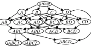
Figure 1(a) shows a partial Bayesian network that carries the belief that the parent concepts of

ABCD are AB and CD. Nodes iA1 and iA2 represent the correctness of students’ responses to two

test items for concept A. In this network, we do not show item nodes for all of the concepts to main-tain the readability of the network. Figure 1(b) shows a Bayesian network that carries the belief that the parent concepts of ABCD are A, B, C, and D. These are the two cases for learning the addition of fractions in Section 1.

2.2 Representing Competence Patterns with GC Matrices

Students’ item responses should relate to their competence levels in concepts. We assume that students have different competence patterns over the concepts inΨ , and adopt matrices to repre-sent the competence patterns of students who belong to different types. Because the format is simi-lar to the Q matrices that Tatsuoka (1983, 1995) used to encode the relationships between the test items and the tested concepts, we name our matrices as GC matrices.

iAB2 iAB1 iD1 iD2 iA1 iA2 C B D A iCD1 iCD2 CD ABCD AB iABCD2 iABCD1 _(a) ABCD iABCD1 iABCD2 C B D A (b) Figure 1. (partial) Bayesian networks for (a) AB~C~D (b) A~B~C~D

Table 1. A GC matrix with only two types of students

group A B C D AB AC AD BC BD CD ABC ABD ACD BCD ABCD

g1 1 1 1 1 1 1 1 1 1 1 1 1 1 1 1

Table 1 shows a GC matrix that specifies competence patterns for only two types of students. The leftmost column shows the names of the types, and the headings of other columns show the names of concepts. The semantics of the contents of the cells depend on whether the concepts are basic or composite. Let qi,j denote the cell at the intersection of i-th row and j-th column in a GC

matrix. If qi,j is 1 and the heading of the j-th column is a basic concept, then the i-th type of student

is competent in the basic concept with a high probability. If qi,j is 1 and the heading of the j-th

col-umn is a composite concept, then the i-th type of student is competent in integrating the parent concepts of the composite concept with a high probability. In both cases, a “0” in the cells suggests a low probability. Note that, when the column heading is a composite concept, a “1” in the cell does not imply that the corresponding type of students is competent in the composite concept. This type of students may not be competent in the composite concept, if they lack the competence in the par-ent concepts. (In other words, a “1” for basic concepts represpar-ents competence, but a “1” for com-posite concepts denotes just the ability to integrate parent concepts.) The contents of our GC matri-ces are related both the rule nodes and the rule application nodes that Martin and VanLehn (1995) defined. We will discuss how we control the ranges of the probability values in Section 2.3.

Without considering the uncertain factors such as guess and slip, the students of the first type in Table 1 are competent in all of the concepts. The students of the second type lack competence in some concepts. Since the composite concepts that involve only two basic concepts must be learned directly from the basic concept, we can infer the competence levels of students based on the infor-mation in a GC matrix. Therefore, we can infer that students of the second type will not be compe-tent in AC because they lack the competence in C, although they are compecompe-tent in integrating the parent concepts of AC.

Note that the contents of GC matrices do not provide sufficient information for us to infer whether a student is competent in composite concept that involves three or more basic concepts. A “1” for a composite concept that covers three or more basic concepts just indicates that typical stu-dents of that group are competent of integrating the parent concepts of that composite concept. Whether typical students of that group are really competent in the composite concept depends on whether the students are competent in the required parent concepts. Take the type g2 in Table 1 for instance. Although this type of students is competent in integrating the parent concepts of ABC with a high probability, the students will be competent in ABC with a low probability because they are not competent in C with a high probability. In contrast, we cannot tell whether students of g2 are competent or incompetent in ABD. We need the GC matrix and the learning patterns for this task. Had we known that the parent concepts of ABD were AD and B, then we would be able to tell that students of g2 would have a low probability of being competent in ABD. Had we known that the parent concepts of ABD were AB and D, then we would be able to tell that students of g2 would have a high probability of being competent in ABD. The GC matrix alone does not provide com-plete information about whether a student is competent in ABD.

We employ a special node, the group node, to represent types of students in a Bayesian net-work. The group node can take on any value that represents a type of student in the study, i.e., g1 or

g2. Since students’ competence in concepts must be influenced by their types, there is a link from

the group node to every concept node. We allow a student to perform differently from the stereo-typical behavior of the student’s group, and control the probability of such a deviation by a simula-tion parameter, β, that is explained in the next subsection.

2.3 The Simulator

We employ the simulator that was invented for a previous work on student classification, so we will not explain the functions of the simulator in great detail. Interested readers are referred to (Liu, 2005).

The simulator takes as input a Bayesian network structure, a GC matrix, and two controlled parameters to produce item responses of a selected number of students. We must create the condi-tional probability tables (CPTs) for every node in the Bayesian network to make it functioning.

There are three types of nodes in our Bayesian networks: the node that represents types of students (called the group node, henceforth), the concept nodes, and the item nodes.

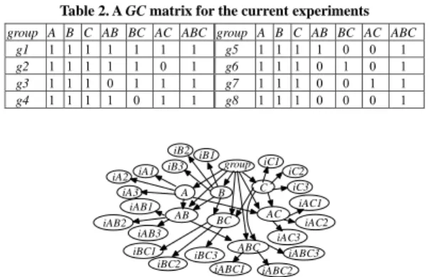
Figure 2 shows a network structure for representing a possible way of learning ABCD (i.e., ABC~D). The structure only shows the group node, the concept nodes, and two item nodes to main-tain the clarity of the network. Not all of the item nodes are included, and the links from the group node to the composite nodes are not shown either. The structure of Figure 2 is employed in our ex-periments to examine the feasibility of the proposed method for model selection, and we do not have a specific interpretation for the concept nodes in the network.

We can simulate any prior distributions for the group node. At this moment, we assume that a student can belong to any of the types in the given GC matrix with equal probabilities. We employ the noisy-and models (Pearl, 1988) for the CPTs of the nodes for composite concepts. The CPTs for the item nodes and the concept nodes for basic concepts have only one parent node, so it is simple to create CPTs for these nodes based on the values of the controlled parameters that we explain next.

The first controlled parameter, α, confines the range of the probabilities of guess and slip. For

instance, if we set α to 0.1, the probability of observing guess and slip will be between [0, 0.1].

The actual probability is chosen with a random number generator that selects a number from the uniform distribution between 0 and α. The second controlled parameter, β, controls the range of the

probability of a student’s performance deviating from the competence pattern of the type that s/he belongs to (Tatsuoka & Tatsuoka, 1997; Table 2). It works in ways that are similar to how the value

of α affects the probability of observing guess and slip. For instance, if we set β to 0.2, a student

may deviate from the standard competence pattern with a probability that is chosen uniformly from the range [0, 0.2]. Note that, although the values of α and β influence the item response pattern of a

simulated student, α and β carry different semantics, and their co-existence allows us to control the

uncertainty of different sources. The actual values in the CPTs of all of the concept nodes and the item nodes are computed based on the samples that are sampled independently from the specified ranges.

After constructing the CPTs for all of the nodes in the Bayesian network, we can compute the conditional probability of answering to a test item correctly given a student type, and use this in-formation to simulate whether a student actually answer correctly or incorrectly with a simple Monte-Carlo method. For instance, assume that we evaluate the Bayesian network and find thatPr(iABC1=correct|group=g2) is equal to 0.6. Since a student must respond to a test item either correctly or incorrectly in our current study, we sample uniformly a number from the range [0, 1], and determine that a particular student responds to iABC1 correctly if this random number is less or equal to 0.6. If this random number is larger than 0.6, we will determine that this student fails to answer correctly. More importantly, we sample a new random number for each test item and for each simulated student, so the simulated results are independent among all of the test items and among all of the students.

3. Motivating Examples and Problem Complexity

Given a GC matrix, the values of α and β, and a network structure, we can simulate the item

responses for a population of students. To examine the applicability of a machine-learning method, group CD BD BC AD AC AB C B D A

ABC ABD ACD BCD iABC2

iABC1 ABCD

a manuscript submitted to Behaviormetrika 7/19 we may then try to recover the network structure by using the simulated data as the input for an algorithm for structure learning.

In this example, we consider only three basic concepts (cA, cB, and cC) and four composite concepts (dAB, dBC, dCA, and dABC). Table 2 shows the GC matrix with which we generated the item responses for 10000 simulated students. In this illustrative example, we used the AB~C pattern (shown in Figure 3), and set both α and β to 0.1. With the item responses created under this setting,

we applied the PC algorithm implemented in Hugin (http://www.hugin.com) to learn the structure of the original network. We manipulated the information available to the PC algorithm to emulate the situations of whether we have non-observable data in the input data to the algorithm. The first obvious choice is to provide complete information about all the nodes to the learning algorithm; and the second is to provide only the information that is truly observable. Namely, in the second alter-native, we provided only the information about the item responses. In a normal situation, without human intervention or tagging, we do not know the states of the group node and the nodes for the competence, i.e., AB, BC, AC and ABC.

Figure 4 shows the network structures that the PC algorithm inferred from the test data. (The nodes were relocated for readability from the network that was generated by Hugin. We attempted to minimize the intersection of links and to move nodes of similar nature close to each other.) We obtained part (a), when we used the complete information, and part (b), when used only the ob-servable information. When we ran the PC algorithm, we set the level of significance to 0.05, which is the default value in Hugin and was also adopted by Vomlel (2004).

Figure 4(a) is not very similar to the original network in Figure 3, which we used to create the simulated data. The nodes for test items are directly connected to their parent concepts, though in diverse directions. The PC algorithm chose to connect the nodes for the concept in ways that we

Table 2. A GC matrix for the current experiments

group A B C AB BC AC ABC group A B C AB BC AC ABC g1 1 1 1 1 1 1 1 g5 1 1 1 1 0 0 1 g2 1 1 1 1 1 0 1 g6 1 1 1 0 1 0 1 g3 1 1 1 0 1 1 1 g7 1 1 1 0 0 1 1 g4 1 1 1 1 0 1 1 g8 1 1 1 0 0 0 1 group C A B AB ABC AC BC iABC2 iABC1 iA1 iA3 iA2 iB1 iB2

iB3 iC1 _iC2 iC3 iAB3 iAB2 iAB1 iAC1 iAC2 iAC3 iBC3 iBC1 iABC3 iBC2

Figure 3. A complete network for the case of learning ABC with AB~C

(a) (b)

Figure 4. Two structures learned with the PC algorithm under different assumptions

a manuscript submitted to Behaviormetrika 8/19

cannot fully justify based on the intended meaning of those concept nodes. Nodes related to the concept ABC were just remotely related to nodes related to the concept C.

In Figure 4(b), the nodes for test items were not connected to the nodes for the concepts be-cause the information about the group node and the concept nodes are completely missing. A ture like part (b) is called item-to-item knowledge structures by (Desmarais et al., 2006). The struc-ture showed close relationships between nodes for test items for ABC and AB, and there was a di-rect relationship between iABC1 and iC3. However, it is hard to tell the relationships among ABC,

AB, and C from this tem-to-item knowledge structure.

We repeated the same procedure for the learning pattern AC~B. Figure 5 shows the network structure which we used to create simulated data. Thicker links emphasize the change in the learn-ing pattern this network structure suggests. We reused the GC matrix shown in Table 2, and set α

and β to 0.1 again. Figure 6 shows the network structures that the PC algorithm learned when the

information about all the nodes (part (a)) and when the information about the observable nodes were provided (part (b)).

Results of such pilot experiments showed that directly applying the machine learning methods may not help us rebuild the network structures very well. The problem is particularly challenging when we have a few completely unobservable nodes in the network. Completely unobservable nodes make it difficult to figure out the relationships among them as Figures 4(b) and 6(b) indi-cated.

Due to such an observation, we attempt to apply the machine learning methods to help the domain experts select the best network structure from a set of candidate structures. This approach is applicable when we have a set of candidate networks in mind, e.g., (Gierl et al., 2007; page 251), and would like to use real data to find the best network.

In the current study, we assume that students learn composite concepts from parent concepts that do not share any common basic concepts. Hence, for instance, ABC and CD cannot serve as the parent concepts of ABCD because they share the basic concept C. This assumption makes the space of possible solutions much smaller than it can be.

Therefore, the number of different ways to learn a composite concept depends on the number of the basic concepts that the composite concept contains, and is related to the Stirling number of type 2 (Knuth, 1973). Assume that we are studying the learning pattern for a composite concept that

group C A B AB ABC AC BC iABC2 iABC1 iA1 iA3 iA2 iB1 iB2

iB3 iC1 _iC2 iC3 iAB3 iAB2 iAB1 iAC1 iAC2 iAC3 iBC3 iBC1 iABC3 iBC2

Figure 5. A complete network for the case of learning ABC with AC~B

(a) (b)

involves λ basic concepts. There are Ω(λ), shown in (3.1), ways to learn this composite concept

(Liu, 2008). The value of Ω(λ) grows very quickly with λ. For example, when λ is equal to 3, 4, 5,

and 6, Ω(λ) is equal to 4, 14, 51, and 202, respectively.

∑ ∑

The quantity prescribed in formula (3.1) is not yet the worst case scenario. When we consider the task of building a model that includes λ basic concepts, there can be S(λ), given in formula (3.2),

different models. Here, λ is not smaller than 3 because it does not make too much sense to discuss

the learning patterns for only two basic concepts.

∏

Finding the best model from this humongous amount of candidate models purely based on only computational requirements might not be very fruitful. This is suggested by the motivating examples that we showed at the beginning of this section. Allowing domain experts to provide a few meaningful candidate models and employing computational techniques to compare these can-didates offer a chance for us to identify a good model for complex problems.

4. Model Selection

We discuss our methods for assisting teachers to select the learning pattern from a set of can-didate answers in this section. Experimental results will be presented in the next section.

4.1 Using Mutual Information as Scores for Candidate Models

Consider the sample network shown in Figure 2 again. Let CI(X, Y, Z) denote the situation that

X and Z are conditionally independent given Y, where X, Y, and Z are three sets of variables. If we

have access to the exact information about the concept nodes, we may choose the learning pattern relatively more easily. In Figure 2, we should have CI({A, B, C}, {ABC, D}, {ABCD}). If the parent nodes of ABCD were AB and CD in Figure 2, then we would have CI({A, B, C, D}, {AB, CD}, {ABCD}), and we will have precise criteria for judging the fitness of network structures when we have information about the concept nodes. In fact, however, we can collect only the item responses that are probabilistically related to the states of the concept nodes, so we do not have ways to de-termine whether CI({A, B, C, D}, {AB, CD}, {ABCD}) holds or not.

Observe the network structures shown in Figure 1 and Figure 2. We can see that the item nodes are linked directly and only to their parent nodes, so, intuitively, item nodes for concept nodes that are more closely related may be more closely related to each other than to item nodes for other concept nodes. For instance, if the actual learning pattern is ABC~D, as shown in Figure 2, then the correctness of answers to test items for ABCD may be more related to the correctness of answers to the test items for ABC and D than to the correctness of answers to the test items for other concept nodes.

We embody the concept of “more related” with the mutual information between two sets of random variables (Cover & Thomas, 2006). Let X and Y denote two sets of random variables, Eq. (4.1.1) shows the mutual information between X and Y, where X) and Y) represent the sets of the possible values of X and Y, respectively. It is easy to prove that, if MI(X;Y)>MI(Z;Y), then knowing the information about X will reduce more uncertainty about Y than knowing the information about Z. Specifically, we have MI(X;Y)>MI(Z;Y) ⇒ H(Y|X)<H(Y|Z), where H(·|·) represents the conditional entropy.

∑ ∑

Consider a more concrete example with the networks in Figure 1 and Figure 2. If

) ; , , , (ABCDABCD

MI is larger than MI(ABC,D;ABCD), we may believe that the learning pattern

A~B~C~D is more likely to be the answer than ABC~D, and the network shown in Figure 1(b) is a better choice than the network shown in Figure 2.

Having chosen this measure, we face the problem of how we can compute the necessary mu-tual information. Recall that we do not know the acmu-tual states of the concept nodes, which are re-quired in applying Eq. (4.1.1). This time, however, we can use the item responses for the concept nodes to estimate the states of the concept nodes, because we are just computing mutual informa-tion not judging condiinforma-tional independence.

We note that using item responses to estimate the states of competence levels is not a perfect choice, though item responses are the most direct observation we have about student’s competence levels. When students respond to a test item correctly, we are not really sure that they are competent of the related concepts. In addition, when students are competent in certain concepts, we are not sure how they will apply these concepts in tests. Hence, there is really a great deal of uncertainty between students’ item responses and their competence levels as we have mentioned in this paper and elsewhere in the literature.

We assume that, in a certain examination, we use n test items to evaluate the competence lev-els of every concept being tested. We also assume that students will respond to every test items in the examination. Figures 3 and 5 show two such examples. In both cases, we have three test items for every concept, i.e., n=3 for all concepts. We also assume that every student will respond to each of these test items, without leaving any of the test times unanswered. Hence, the portion of correct responses to the test items for a concept must be one of {0, 1/n, 2/n, …, 1}, and we can use this portion as an indication of the competence level of the concept. (If different concepts have different numbers of test items, we can adapt this estimation procedure by considering this factor accord-ingly.) We can generalize this estimation method for a set of concept nodes, and Eq. (4.1.2) shows an example. students of number for items test 2 and for em it test 1 to correctly respond who students of number ) / 2 , / 1 Pr( BC A n BC n A= = = (4.1.2) To avoid the problem of zero probability values that are caused by rarely observed cases in the simulation, we add a very small amount to the counts of basic events to smooth the probability distributions. Currently this small number is 0.001.

After estimating the marginal and joint probability distributions of concept nodes, we can ap-ply Eq. (4.1.1) to compute the mutual information of interest, and use the results as the scores of the learning patterns. When λ is 4, we will have to compute a score for each of the 14 learning patterns as dictated by formula (3.1).

4.2 Using Supervised Learning for Model Selection

Experimental results, which are provided in a later section, indicated that using mutual infor-mation as the scores for the learning patterns can be useful. However, there are situations when us-ing mutual information alone could not help us achieve high performance. Recall that we do not have the actual probability distributions of the concept nodes, so we have to use the item responses to estimate these distributions. Consequently, when the relationship between the correctness of item responses and the competence of individual concepts is really uncertain, our estimation can become quite inaccurate. For instance, when the largest and the second largest scores for the learning pat-terns were quite close, e.g., the ratio was less than 1.2, it was quite common that the raw values of the mutual information did not lead us to the correct answer.

Hence we would like to introduce more features when we apply the machine learning tech-niques to find the best learning pattern. The previous experience suggests that collecting the ratio between each of the original mutual information and the largest original mutual information can be

a manuscript submitted to Behaviormetrika 11/19 useful. In addition, the ratio between the largest score and the second largest score and the ratio between the largest score and the average score are also useful. Take the study for the learning pat-tern of ABCD as an example. In addition to the original 14 scores, we obtain 14 ratios between these original scores and the largest score. We also divide the largest score by the second largest score and divide the largest score by the average score to get two more features. Therefore we have 30 features in total. (Note that we did not manually set thresholds for these ratios. Mentioning the value of “1.2” in the preceding paragraph was meant to bring to readers’ attention the usefulness of ratios between raw features.)

In summary, when we have some candidate learning patterns in mind, we can generate simu-lated data with the learning patterns, a GC matrix, and the controlled parameters. Since the learning patterns are known when we generate the simulated data, the learning patterns can be used as the class labels in supervised learning (Witten & Frank, 2005). We can create training instances by as-sociating the features with class labels to train a classifier, use the classifier to classify the item re-sponses of real students, and use the classification result as the learning pattern of the real students. Based on this principle, we can apply support vector machines (SVMs) (Cortes & Vapnik, 1995), artificial neural networks (ANNs) (Bishop, 1995), or any other appropriate classification techniques in our experiments. Experimental results observed in some early explorations showed that we achieved results of similar quality when we used appropriate parameters for the right SVM or ANN models (Liu, 2008). In the next section, we choose to report results of using SVMs in our classifi-ers.

5. Experimental Studies

In the current study, we assume that all of the students learn a composite concept with the same learning pattern. This allows us to find the candidate pattern that has the highest score and to simplify the procedures of our experiments. If we will consider multiple learning patterns, say k learning patterns, for a composite concept in other experiments, we just have to choose those k can-didate patterns with leading scores.

Because we did not collect students’ data in a real scenario, we use only simulated data in this study, and employ a Bayesian network to represent the true learning pattern. We try to find the learning pattern for ABCD in the experiments. We assume that there are professional sources that can provide us the list of candidate learning patterns, and we can represent each of these candidates with a corresponding Bayesian network. We assume that our professional advisors can provide per-fect information about the GC matrix, which contains information about students’ competence pat-terns. With a Bayesian network, a GC matrix, and two controlled parameters, we can generate simu-lated data as explained in Section 2.3. After generating the training and test data with due proce-dures, we can conduct experiments and record the accuracy achieved by our classifiers.

5.1 Bayesian Networks for the Experiments

We conducted five sets of experiments. Each of these experiments uses one pattern in {A~BCD, AB~CD, A~BC~D, A~B~CD, A~B~C~D} as the true learning pattern. These patterns are selected to represent different ways of combinations of the parent concepts of ABCD. A~BCD and AB~CD rep-resent two different ways to learn ABCD with two parent concepts. They are different because one parent concept in A~BCD has only one basic concept, and, in contrast, both parent concepts in AB~CD have two basic concepts. Using an intuitive interpretation of “similarity”, A~BC~D and A~B~CD are two similar ways to learn ABCD with three parent concepts. A~B~C~D represents the direct integration of four basic concepts into the composite concept.

Note that it can be difficult to tell the differences between the item responses of students who employ closely related learning patterns. A~BC~D and A~BCD are closely related because A~BC~D is refined form of A~BCD by splitting BCD into BC and D. Analogously, A~B~CD and A~BCD are closely related, and A~B~CD and AB~CD are closely related. Hence, we believe that we have

cho-a mcho-anuscript submitted to Behcho-aviormetrikcho-a 12/19

sen a challenging task for our tests.

In order to make our classifier have a chance to find the correct learning pattern, we assume that some professional teachers will provide {A~BCD, AB~CD, A~BC~D, A~B~CD, A~B~C~D} as the list of candidate solutions. Namely, we make sure that the list includes the true learning pattern, no matter which of the learning patterns that we discussed at the beginning of this subsection is used as the true learning pattern.

In all of our experiments, we assume that the parent concepts of ABC, ABD, ACD, and BCD are basic concepts. Other situations are discussed in the third paragraph in Section 6. Given this assumption and the learning patterns, we can construct the structures of the Bayesian networks that our simulator needs.

5.2 The GC matrices and Controlled Parameters

In addition to the network structures, our simulator needs a GC matrix that specifies students’ competence patterns. When we are using simulated data in the experiments, we need two GC ma-trices. One represents the competence patterns that we obtain from the professional sources, and the other represents students’ actual competence patterns. When the professional sources are highly experienced, we may be able to obtain an accurate GC matrix. Hence, we use only one GC matrix for generating the training and test data in our experiments for now.

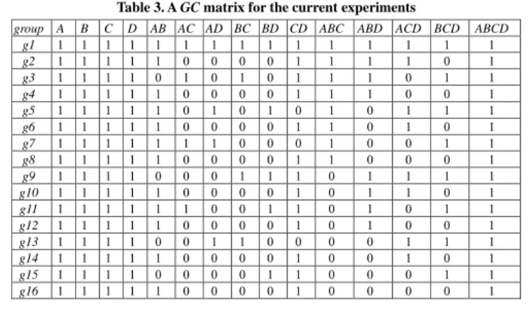
Table 3 shows the GC matrix that we used in our experiments. We use the same format that we used in Table 1 to present a GC matrix in Table 3. This GC matrix was also used in experiments in which a different list of candidate patterns was used (Liu, 2008), so it is possible to compare the experimental results.

There are 16 types of students in Table 3, and we can examine the settings for different types of students. All of these 16 types of students are capable of using A~B~C~D as their learning pat-tern. When i is an odd number, students of types gi can use A~BCD. Students of types gi, i = 1, 2, 4, 6, 8, 10, 11, 12, 14, and 16, can use AB~CD; students of types gj, j = 1, 3, 9, and 13, can use A~BC~D; and students of types gk, k = 1, 2, 3, 4, 6, 8, 9, 10, 11, 12, 14, 15, and 16, can use A~B~CD.

We can also examine the settings for different concepts. All of these 16 types are capable of the basic concepts and are capable of integrating the parent concepts of ABCD. If we want to study how students learn ABCD, we should recruit students that appear to be competent in ABCD in our study, so the settings in the A, B, C, D, and ABCD columns should be reasonable. Treating ABC,

ABD, ACD, and BCD as a group, we have 16 possible ways to set the values for this group, and we

do that in Table 3, which is an important reason why we have 16 types of students in Table 3. There Table 3. A GC matrix for the current experiments

group A B C D AB AC AD BC BD CD ABC ABD ACD BCD ABCD g1 1 1 1 1 1 1 1 1 1 1 1 1 1 1 1 g2 1 1 1 1 1 0 0 0 0 1 1 1 1 0 1 g3 1 1 1 1 0 1 0 1 0 1 1 1 0 1 1 g4 1 1 1 1 1 0 0 0 0 1 1 1 0 0 1 g5 1 1 1 1 1 0 1 0 1 0 1 0 1 1 1 g6 1 1 1 1 1 0 0 0 0 1 1 0 1 0 1 g7 1 1 1 1 1 1 1 0 0 0 1 0 0 1 1 g8 1 1 1 1 1 0 0 0 0 1 1 0 0 0 1 g9 1 1 1 1 0 0 0 1 1 1 0 1 1 1 1 g10 1 1 1 1 1 0 0 0 0 1 0 1 1 0 1 g11 1 1 1 1 1 1 0 0 1 1 0 1 0 1 1 g12 1 1 1 1 1 0 0 0 0 1 0 1 0 0 1 g13 1 1 1 1 0 0 1 1 0 0 0 0 1 1 1 g14 1 1 1 1 1 0 0 0 0 1 0 0 1 0 1 g15 1 1 1 1 0 0 0 0 1 1 0 0 0 1 1 g16 1 1 1 1 1 0 0 0 0 1 0 0 0 0 1

are a total of 64 possible ways to set the capabilities of integrating concepts that include two basic concepts, but we have chosen 16 of them arbitrarily in Table 3.

In Section 2.3, we explained how we use the controlled parameters α and β to modulate the

ranges of slip and guess and to manipulate the possibility of students’ deviation from the standard competence patterns of their types. Both α and β can be set to any value from {0.05, 0.10, 0.15,

0.20, 0.25, 0.30}. We do not try values that are larger than 0.30 because those situations are really rare and were not discussed in the literature. As a result, for any pair of a network structure and a

GC matrix, we repeat the experiment 36 (=6×6) times.

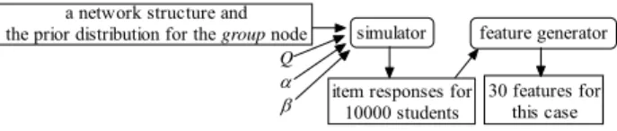
5.3 Main Steps of the Experiments

Figure 7 shows the flow that we employed to create an instance of datum for our experiments. Given a network structure along with the prior distribution for the group node, a GC matrix, and a particular combination of α and β, we used the simulator that we described in Section 2.3 to create

item responses of 10000 students. We assumed that students responded to three test items for every concept in the experiments, but this quantity could be changed easily. With the item responses, we applied the methods that we described in Section 4.1 to estimate the mutual information and to compute the derived features.

In the experiments, we repeated this procedure 600 times for every possible solution in {A~BCD, AB~CD, A~BC~D, A~B~CD, A~B~C~D}, the GC matrix in Table 3, and all of the 36 pos-sible combinations of α and β. The conditional probability tables were re-sampled for every one of

these 600 instances, so their underlying probability distributions were mutually independent given the setups of the experiments. Hence, for any combination of α and β, we had 600 instances for a

possible learning pattern. We could use 500 instances for every learning pattern to train our classi-fier, and used the remaining 100 instances as the test data. In total, we had 2500 training instances and 500 test instances when we ran an evaluation of our approach.

We employed LIBSVM (Chang & Lin, 2001) for realizing our classifier. We chose the SVMs of type c-SVC, and used the radial basis function as the kernel function. Since there were still free parameters in the SVMs, we had to run some explorative tests to search the best combination of the parameters C and γ in LIBSVM. In these explorative tests, we set C and γ to any value in {0.1,

0.2, …, 1.9}, so we had to run 361 explorative tests. We used the training data as the test data to search the combination of C and γ that helped us achieve the highest accuracy in these explorative

tests. This particular combination of C and γ was then used in the evaluation that used the real test

data.

5.4 Preliminary Analysis

It was possible for us to use the original 14 mutual information, which we discussed in Section 4.1, to guess the learning patterns. A simple procedure was just to select the learning pattern that corresponded to the largest mutual information, and it was easy to verify whether the procedure found the correct pattern because each instance of datum was labeled with the correct learning pat-tern. Since we had a total of 3000 instances for every combination of α and β, we could use the

proportion of correct identification as the accuracy for this simple procedure.

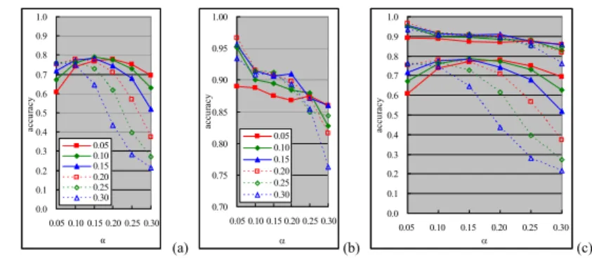
Figure 8(a) shows the results of such experiments for all of the combinations of α and β. The

vertical axis shows the accuracy, the horizontal axis shows the values of α, and the legend shows

simulator item responses for

10000 students feature generator 30 features for this case Q α β

a network structure and the prior distribution for the group node

Figure 7. Generating an instance of datum for the experiments

the values of β. Although using only mutual information for determining the learning patterns can

perform well in some cases, the trends of the curves show that the results can change radically with the varying α and β. When α and β are both 0.3, the accuracy is just 0.2.

Note that this result of 0.2 was not due to that the simple procedure randomly selected an an-swer from five possible anan-swers. This simple procedure did not know that there were only five pos-sible answers. It was allowed to guess any of the pospos-sible answers—14 pospos-sible answers when λ

was 4. This phenomenon was due to the similarity among the competing concepts. For instance, when α was small, this simple procedure frequently chose AD~BC as the answer for test instances

that had A~BC~D as their labels. A procedure that randomly selected an answer from 14 candidates would have led to the result of about 0.0714 in accuracy. The reason for the result of 0.2 was be-cause, when α and β were large, the simple procedure inclined to select A~B~C~D as the learning

pattern. This should not be very surprising because all of the concepts must be related to the basic concepts. Because A~B~C~D was used in 600 instances, we had about 600 correct answers out of 3000 test instances in the experiments, making the accuracy about 0.2.

5.5 Experimental Results

Figure 8(b) shows the results that we achieved by using the SVM-based classifiers to guess the learning patterns. The horizontal axis, the vertical axis, and the legend in Figure 8(b) carry the same meaning as their counterparts in Figure 8(a). Figure 8(c) shows all of the curves in Figures 8(a) and 8(b) in one chart to help us compare the experimental results.

The chart in Figure 8(b) indicates that the accuracy achieved by our classifier still depends on the values of α and β. The trends of the curves also suggest that the accuracy reduced as we

in-creased the values of α and β. However, this relationship does not hold all the time, and we will see

an example in the next subsection. There are other factors which influence the observed accuracy. The chart in Figure 8(c) shows that we improved the accuracy a lot by using the do-main-specific information to train a classifier and by using this classifier to judge the unobservable learning pattern from the item responses. The positions of curves that we copied from Figure 8(b) lie above their counterparts that we copied from Figure 8(a). In addition, we reduced the variation in accuracy by using the classifiers.

We also used the F measure (Witten & Frank, 2005) to gauge the quality of our classifiers, in addition to using the proportion of correct classification as the measure for the quality. Since we classified the test instances into one of five candidate answers and the true answer of every test in-stance belonged to the five candidates, we could calculate the precision and recall (Witten & Frank, 2005) for each of the five classes. To obtain the F measure for an experiment, we calculated the average precision based on the precision for the five classes, and calculated the average recall

0.0 0.1 0.2 0.3 0.4 0.5 0.6 0.7 0.8 0.9 1.0 0.05 0.10 0.15 0.20 0.25 0.30 α acc ur ac y 0.05 0.10 0.15 0.20 0.25 0.30 (a) 0.70 0.75 0.80 0.85 0.90 0.95 1.00 0.05 0.10 0.15 0.20 0.25 0.30 α ac cu racy 0.05 0.10 0.15 0.20 0.25 0.30 (b) 0.0 0.1 0.2 0.3 0.4 0.5 0.6 0.7 0.8 0.9 1.0 0.05 0.10 0.15 0.20 0.25 0.30 α ac cu ra cy (c) Figure 8. Domain-specific constraints improve the classification accuracy