在液態鎵模型中結構次序之量化

國

立

交

通

大

學

物理研究所

碩

士

論

文

在液態鎵模型中結構次序之量化

Quantification of structure order in a model of liquid Ga

研 究 生：陳琳元

指導教授：吳天鳴 教授

在液態鎵模型中結構次序之量化

Quantification of structure order in model of liquid Ga

研 究 生：陳琳元 Student：Lin-Yuan Chen 指導教授：吳天鳴 教授 Advisor：Ten-Ming Wu

國立交通大學

物理研究所

碩士論文

Submitted to Institute of Physics College of Science

National Chiao Tung University in partial Fulfillment of the Requirements

for the Degree of Master

in

Physics

July 2010

Hsinchu, Taiwan, Republic of China

在液態鎵模型中結構次序之量化

學生：陳琳元 指導教授：吳天鳴 教授

國立交通大學物理研究所碩士班

摘要

為了量化描述物質結構在影像上資訊的數學參數，包括可以了解整體性 的結構次序的 oreintational order parameter 和 translational order

parameter，可以判別固體堆垛的 local orientational order parameter，我們 利用這些參數來探討在不同熱力學狀態下，液態鎵模型的系統結構次 序。Orientational order parameter 可以了解整體性的結構次序，translational order parameter 探討系統在長距離內平移性結構次序，而 local orientational order parameter 可探討區域性結構次序，並當成協助判斷固體堆跺的方 法。我們探討了在不同溫度、密度下結構參數以及固體堆垛形成，並探 討了 Friedel oscillations 的影響。

Quantification of structure order in model of liquid Ga

student：Lin-Yuan Chen Advisors：Dr. Ten-Ming Wu

Institute of Physics

National Chiao Tung University

ABSTRACT

In this thesis, in order to quantitatively describe the structure order in a model of liquid Ga, several order parameters have been used, including translational order parameter and orientational order parameter, which characterize the global structures, and the local orientational order parameter, which is used to analyze the cluster formation. In terms of these order parameters, we

investigate the structure orders of the model potential at various

thermodynamic states. For the model and the repulsive core only of the model, the variations of these order parameters and the cluster formation with

temperature and densities are presented, so that the effects due to the Friedel oscillations are obtained and discussed.

誌 謝

Contents Abstract (Chinese)………..……….i Abstract (English)………ii Acknowledgement………...………iii Content ……….………...iv Figure Captions………vi Chapter 1 Introduction………..……….1

Chapter 2 Model of liquid Ga and MD simulation ……….………2

Chapter 3 Static structure factor, Order Parameters and Cluster Analysis 3-1 Radial distribution function………...……..4

3-2 Static structure factor ……….……….4

3-3 Translational order parameter………..5

3-4 Orientational order parameter………..5

3-5 Local orientational order parameter……….…………..….…6

3-5-1 Threshold value for Cluster Formation…….………...8

Chapter 4 Numerical Results and Discussions………..………9

4-1 Variation of structures with density at T=323K………...9

4-1-1 Translational order parameter……….….…….9

4-1-2 Orientational order parameter……….……..…9

4-1-3 Order map……….…………9

4-1-4 Clusters of Full potential ……….……..…10

4-1-5 Clusters of Repulsive core only ……….………11

4-2 Variation of structures with temperature at densityρ=3.305.11 4-2-1 Translational order parameter……….………12

4-2-3 Order map……….………..12

4-2-4 Clusters of Full potential ………...12

4-2-5 Clusters of Repulsive core only ………13

Chapter 5 Conclusions………..…..14

Figure Captions

Figure. 1. Static structure factor for liquid Ga at 323K ρ=3.305 ……...1 Figure. 2. Interatomic pair potential of liquid Ga……..….……..………2 Figure. 3. Repulsive core potential………..….………2 Figure. 4. Cubic box with all side length L and N particles inside ...…...3 Figure. 5. Full potential, Isolated particle number variation with density for

Kc=0.5,Kc=0.7 and Kc=0.9………..…………..……...8

Figure. 6. Variation of translational order parameter with density at

T=323K………..……..……..…….16 Figure. 7. Variation of orientational order parameter with density at

T=323K………..…………...17 Figure. 8. (a) Static structure factor of full potential at T=323K

(b) Static structure factor of repulsive core only at T=323K...18 Figure. 9. Order maps of full potential (circles) and repulsive core only

(squares) at T=323K……….……….…….………….19

Figure. 10. Cluster distributions of the full potential with Kc=0.5 and the

cutoff of the bond length at rmin=0.89…...20

Figure. 11. Cluster distributions of the full potential with Kc=0.5 and the

cutoff of the bond length at rmin=1.1………..…...……..21

Figure. 12. Cluster distributions of the full potential with Kc=0.5 and the

cutoff of the bond length at rmin=1.3.………..22

Figure. 13. Cluster distributions of the full potential with Kc=0.5 and the

cutoff of the bond length at rmin=1.5….………...……23

Figure. 14. Cluster distributions of the full potential with Kc=0.5 and the

cutoff of the bond length at rmin=1.76………..…………24

Figure. 15. Density variation of the isolated particle number for the full

potential with the cutoff distance rmin=0.89, 1.1, 1.3, 1.5 and

Figure. 16. The g(r) function of the full potential at T=323K and different density………...…..……26

Figure. 17. Cluster distributions of the repulsive core only with Kc=0.5 and

the cutoff of the bond length atrmin=0.89……….……27

Figure. 18. Cluster distributions of the repulsive core only with Kc=0.5 and

the cutoff of the bond length atrmin=1.1..…….…………..…..28

Figure. 19. The g(r) function of the repulsive core only at T=323K and different density...29 Figure. 20. Distribution of the isolated particles in the full potential (circles)

and the repulsive core only (squares) with rmin=0.89(a) and

min

r =1.1(b)………30

Figure. 21. Temperature variation of the translational order parameter at ρ=3.305 for the models of the full potential (circles) and the repulsive core only (squares)………...…31 Figure. 22. Temperature variation of the orientational order parameter at

ρ=3.305 for the models of full potential (circles) and the repulsive core only (squares)……….…..32 Figure. 23. Static structure factors S(q) of the full potential (a) and the

repulsive core only (b) at ρ=3.305………33 Figure. 24. Order maps for the models of the full potential (circles) and the

repulsive core only (squares) at ρ=3.305 for several

temperatures……….34 Figure. 25. Comparison for the order map of the temperature and density

variations for the models of the full potential and the repulsive core only………..……….35 Figure. 26. Comparison for the radial distribution functions g(r) of the

solids obtained by different simulation process………...36 Figure. 27. The cluster distributions of the full potential at ρ=3.305 and

three temperatures with the cutoff rmin=0.89 (a) and rmin=1.1 (b)

………..37 Figure. 28. The cluster distributions of the repulsive core only at ρ=3.305

and three temperatures with the cutoff rmin=0.89 (a) and

min

r =1.1 (b)………38

Figure. 29. The g(r) function of the full-potential model atρ=3.305 and T=313k, 283K, 173K, 153K and 103K…...……….39 Figure. 30. Temperature variation of the isolated-particle distribution for the

full potential (circles) and the repulsive core only (squares) with

the cutoff at rmin=0.89 (a) and rmin=1.1 (b)………..40

Figure. 31. The difference between the isolated-particle distribution

atrmin=0.89 and rmin=1.1 for the models of the full potential

Chapter 1

INTRODUCTION

As one of the polyvalent liquid metals that are well known for anomalous structures, Ga has many uncommon properties, such as low melting point at

Tm=302K, and a shoulder on the high-q side of first peak of static structure

factor, as shown in Fig.1. The physical reason for this anomalous shoulder is still unknown and gives rise to our curiosity.

Fig.1 Static structure factor for liquid Ga at 323K ρ=3.305 The high-q shoulder can be produced by a model of interatomic pair

potential that is generated by a first-principles theory Ref[1]. The interatomic pair potential includes a repulsive soft core and a long-range oscillatory part, called “Friedel oscillations”. It is concluded that the high-q shoulder may be caused by many ”1201 clusters”. From Ref[2], we know that for the potential with the repulsive soft core only, the high-q shoulder does not appear.

To find out the cause for the high-q shoulder, we need to know more about the potential model in Ref[1] for pure Ga liquid metal and the effect caused by Friedel oscillations on the structure order of the liquid. Computer

simulation results of Ga produce complex structural information, so we use the structure order parameters that are introduced in Ref[3], Ref[4] and Ref[5] to study pure Ga liquid structure. The structure order parameters are a more objective way for describing structure order quantitatively.

20 30 40 50 60 70 q (nm^-1) 1 1.5 2 S(q) 323K density 3.305

Chapter 2

Model of liquid Ga and MD simulation

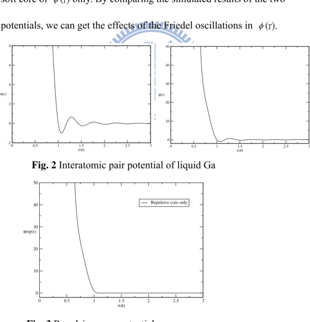
The effective interatomic pair potential(r) of liquid Ga is generated by a

first-principles pseudopotnetial theory Ref[1] and Ref[6]. The potential model contains a repulsive soft core and an oscillatory tail called “Friedel Oscillations”. As shown in Fig. 2, the minimum of the first attractive well is located at 4.32 Å, and first, second and third maxima are located at 5.17Å, 7.15Å, 9.13Å, respectively. Shown in Fig. 3 is another pair potential that we simulate, and is called “the repulsive-core potential”, which is the repulsive

soft core of (r) only. By comparing the simulated results of the two

potentials, we can get the effects of the Friedel oscillations in (r).

Fig. 2 Interatomic pair potential of liquid Ga

Fig. 3 Repulsive-core potential

0 0.5 1 1.5 2 2.5 3 r(σ) 0 10 20 30 40 50 φ(r) 0 0.5 1 1.5 2 2.5 3 r(σ) -2 0 2 4 6 8 φ(r) 0 0.5 1 1.5 2 2.5 3 r(σ) 0 10 20 30 40 50 φrep(r)

Using classical molecular dynamics simulation (MD) and the standard periodic boundary conditions, we simulate N particles interacting with the

effective interatomic pair potential(r) or the repulsive core potentialrep(r) in

a cubic box of length L under constant temperature T (canonical ensemble) with Verlet algorithm Beeman form.

Fig. 4 Cubic box with all side length L and N particles inside In the first part MD with T=323K, we get configurations of system at different densities. The temperature 323K is slightly above the melting

temperature of Ga, so that we can study structures in liquid states. As density increases, the system may be change to a solid state at 323K.

In the second part, the reduced density of the system is fixed at 3.305, which is that of Ga at 323K. We get system configurations at different temperatures.

In our simulations, σ =7.645 au=4.044Å, t0=5.4×10-12s=5.4 ps, r* is real

Chapter 3

Static structure factor, Order Parameters and

Cluster Analysis

3-1. Radial distribution function[PDF, denoted by g(r)]

The radial distribution function (PDF) describing the structures of configuration is calculated as )) ) ( ( 3 4 ( ) ( 3 3 dr r r n r g        (1)

where ρ is density,Δn is the number of particles that are found between distance r and r-dr from a central particle. Also, g(r) needs to satisfy



where N is the total number of particles in the system. g(r) is the local density that the central particle feels at distance r. As r is vary large, we have

g(r)=1,that means the local density from the central particle equals the density of the system.

3-2. Static structure factor

To introduce static structure factor, S(q), we may compare our simulation data with the scattering experimental data. From references, S(q) is defined as

S

(

q

)



1





d

r



exp(

i

k





r



)





(

g

(

r

)



1

)

3-3. Translational order parameter

Although PDF can show the radial behavior of our system, but to give a quantitative expression for structure order, we introduce translational order parameter defined as



 the number density. As r is

scaled with the mean separation of particles, the translational order parameter

can avoid the effects due to system density. sc is a numerical cutoff, and we

set sc to be 2.317851 in our calculation.

For a completely uncorrelated system, g(s) is 1 and thus τ vanishes to zero, but for systems with long-range order, τ is very large.

3-4. Orientational order parameter

As the translational order parameter describes the long-range order of

structures, we introduce orientational order parameter to describe short-range order of structures. For describing short-range order, we need to define the

bonds between particles. The unit vector rˆij representing the direction

pointing from the i-th to the j-th particle is specified by the related polar and

azimuthal angles ijandij. To characterize the bond angles, we use spherical

harmonic functions Y_lm(_ij,_ij),

e

wherePml(x)is the associated Legendre function. The purpose of orientational

order parameter is to quantify short-range order; therefore, a cutoff distance

min

r is required. r_minis usually set as the first minimum position of g(r), to

include the particles within the first-shell structure of a central particle. For a

central particle “i” and ni particles within the cutoff distance rmin,

) , ( 1 1 ij ij n i j lm N i bond lm i Y N Q





is the average of bond spherical harmonic functions, with Nbondbeing the total

number of bonds with central particles. To avoid the effects due to the

coordinate axes we choose, a rotationally invariant order parameterQl is then

an average square sum of different m in Eq.(6) as



In this work, we use Q₆, which decreases as the system becomes less

structural, and increases as the system structure is crystal-like. For example,

for a perfect fcc crystal with 12 first nearest neighbors, ₆fcc 0.5745

Q , and for

a completely uncorrelated system,

bond

N Q₆  1 .

3-5. Local orientational order parameter

For particles within the bond lengthr_min, we sum the spherical harmonic

function of bonds to the i-th particle as





Y

n

i

q

)

,

(

1

)

(





where ni is the local bond number to the i-th particle. Like what we have

done for the orientational order parameter, one can evaluate a rotationally invariant order parameter that quantifies the local structure order associated with the i-th particle as

2 1 2

]

)

(

1

2

4

[

)

(







q

i

l

i

q



Choose l6 for our work. Therefore, any particles in the system have a

complex vector of 261components characterizing the local structure order,

with each component as



The properties of vector-dot product are that for any two normalized vectors in the same direction, their dot product equals 1. For two particles i an j

within the r_min range, with the local orientational order parameter vector-dot

product is greater than a threshold value Kc,

K j q i q j q i q  



we say that the two particles i and j are “Connected”. A cluster is a group of connected particles. So, we use the connect relation between particles to find clusters and determine their sizes. A particle without any connected particles is called an isolate particle, which does not belong to any group clusters. 3-5-1. Threshold value for Cluster Formation

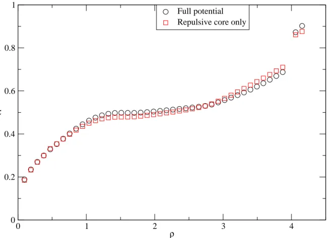
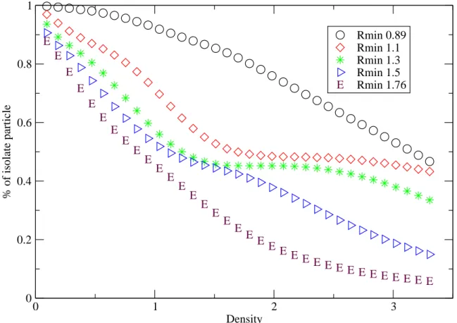
If threshold value Kc of local orientational order parameter is too small, the

effect structure order for distinguishing will be low Ref[5]. The results of

different threshold values Kc for calculating local orientational order

parameter are shown in Fig. 5. For Kc=0.9 and 0.7, very few bonds can be

recognized, and most particles are classified as “isolate particle”(without

connected neighbors). Thus, we choose Kc=0.5 in our study so that the cluster

number is clearly varied with system density.

Fig. 5 Isolate-particle number variation with density at Kc=0.5, Kc=0.7 and

Kc=0.9, for the system of full potential.

2 3 4

ρ

0 0.5 1

Isolate particle number / total particle number

Kc=0.5 Kc=0.7 Kc=0.9

Chapter 4

Numerical Results and Discussions

4-1 Variation of structures with density at T=323K

In this subsection, we examine the variation of simulation results with density

of temperature 323K. The translational order parameter shown in Fig. 6 and

orientational order parameter Q6 in Fig. 7 have the same behavior as in Ref[4].

From g(r) in Fig.16 (f) and S(q) Fig. 8 with Ref[5], Ref[6], we know that our system changes to a glassy state, as the discontinuous jump occurs in the

density variations of  , Q6 and in the order map.

4-1-1 Translational order parameter

Fig. 6 is the quantitative results of the translational order parameter. Both

Full potential and Repulsive core only show the same behavior that

increases with density. For systems at low density, the full-potential system is a little more order than the repulsive-core-only system. At high densities, the repulsive-core-only system is a little more order than the full-potential system.

 has a discontinuous jump at density about 4. We know from Ref[3],Ref[4]

the jump corresponds to the system phase transition from liquid to solid state. This can also be observed from g(r) in Fig. 16. At solid states, the

translational order parameter of full potential is higher than that of the repulsive core only, which shows that Friedel oscillations have a positive effect on the translational order of the structure.

4-1-2 Orientational order parameter

At liquid states, bond orientation of particles are out of order, as in Fig. 7,

and the Q6 value is vary small. At density about 4, Q6 has a discontinuous

jump as that in the translational order parameter. As the system transfers to the solid state, the bond-orientational order is significantly increased, and we can

see from Fig. 7 the Q6 of the full potential is higher than that of the repulsive

core only. This also shows that Friedel oscillations of the full potential have a positive effect on the structure order in the solid states.

4-1-3 Order map

liquid states. In the order map, the solid states are separated from the liquid states. In the solid states, the structures of the full potential are more order in

Q6 than those of the repulsive core only.

4-1-4 Clusters of Full potential

Fig. 10, Fig 11, Fig. 12, Fig. 13, and Fig. 14 show the distributions of

cluster sizes for the full potential with different r_mincutoffs. In Fig. 10 with the

cutoff at r_min=0.89, only the first shell of g(r) shown in Fig. 16 is taken into

account. The size of a cluster and the number of clusters increase as density is increased, as our expectations. From Fig. 16, the first peak of g(r) grows

exactly with density. In Fig. 11 with r_min=1.1, this cutoff includes the second

shell in g(r) that is very close to the first shell of structure, and the clusters keep growing with the increase of density. But at density about 1.8 to 2.6, the cluster distributions are almost the same. This is resulted from the second peak in g(r) lower and the first peak higher, because in this density range the second shell structure starts to be compressed into the first shell and the two shells of structure merge into one. Also from Fig. 6 at the same density region, the translational order parameter is close to be horizontal, which means that the radial structure order of the system does not increase. In Fig. 12, with

min

r =1.3, the distribution of clusters still has a tendency to grow with density.

As density is over 2.8 because part of the third shell as shown in g(r) is included, the clusters grow strongly. But at densities between 1.6 and 2.4, clusters have an anomaly behavior with the local structure order decreasing as density increases. The reason of this behavior is that in this density region as density increases, part of the second shell of the structure is destroyed and classified into different group of the first shell and the third shell. As we can see that the third-shell peak in Fig. 16 gets close to 1.3 but just at the range

out of 1.3. In Fig. 13 with r_min=1.5, again, the clusters grow with density. For

density over 1.7, almost all of the third shell structure are counted in, and thus

the clusters become vary large. In Fig. 14 with r_min=1.76, the cluster behavior

is generally proportional to density. Almost all of the particles in system are recognized as a big cluster. By considering the results of above and Fig. 15 for

the isolate-particle distribution at different densities and cutoffs, a large

min

r will cause a difficulty in comparing the results. Therefore, we take r_min=

0.89 and r_min=1.1 for the works of different potential Ga model simulation

and temperature variation for the full potential and the repulsive core only Ga

model simulation. We can see in g(r), r_min=0.89 is the position that contains

the first shell of the structure, andr_min= 1.1contains the second shell so that we

can know the local order by these two cutoff distances. 4-1-5 Clusters of Repulsive core only

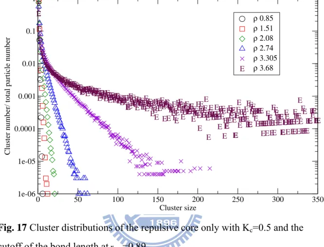
In Fig. 17 and Fig. 18 we show simulation results of the cluster distributions

of the repulsive core only at r_min=0.89 and r_min=1.1, respectively. In Fig. 20,

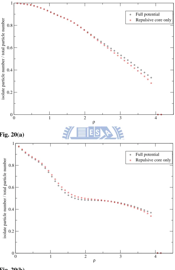
the distribution of isolate particles, which are particles do not connect with any other particles are compared for the two pair potentials we simulated. If

the isolate-particle number is higher, the structure is less order. For r_min=1.1

and density between 2 and 2.7, as density increases, the cluster structures do not follow. This happens to the cases with the full potential and the repulsive

core only, because at r_min=1.1, the system can not distinguish the second shell

from the first shell.

Shown in Fig. 20, we find that for low densities the full-potential model has higher local-structure order than the repulsive core only, and for high densities the situation is reversed. The difference between the two cases should be caused by the Friedel oscillations in the full potential. From g(r) and S(q) for the full potential and the repulsive core only we can see that the main reason that causes the system turn into solid states should be the repulsive core part of the potential, because both models turn into solid states at density about 4.

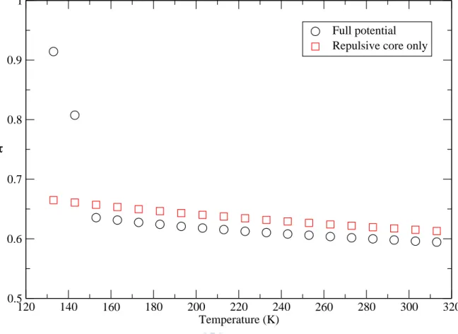
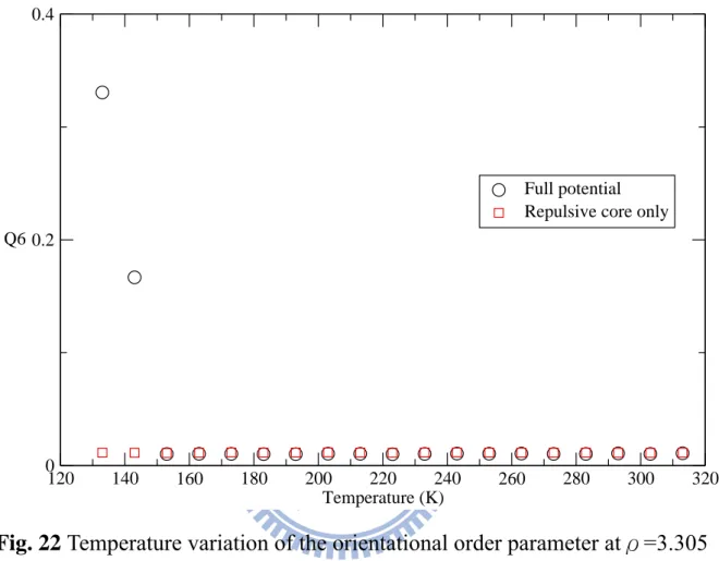
4-2 Variation of structures with temperature at densityρ=3.305

In this subsection, we examine the variation of the simulated structures with temperature at ρ=3.305. The temperature variations of the translational order

parameterτ and the orientational order parameter Q6 are shown in Fig. 21

and Fig. 22, respectively. For the full potential, as temperature decreases a

jump of τand Q6 appears, similar as the one as the density of the system

increase. Compared with S(q) shown in Fig. 23, we show the solid state

similar as the-phase of Ga. This evidences that our temperature variation

MD simulation is correct.

4-2-1 Translational order parameter

The translational order parameter tends to grow very little as temperature is decreased. However, as temperature is lower than about 150K, the system of full potential turns to solids. This can also be evidenced from g(r). We observe

that  has a discontinuous jump. But, for the repulsive core, the translational

order parameter does not have a discontinuous jump. The main reason that the system of the full potential turns to solid in the quenching process should be due to the Friedel oscillations of the full potential.

4-2-2 Orientational order parameter

For Q6 in Fig. 22, again, the full potential has a discontinuous jump similar

as one in the translational order parameter. From the behavior of these two order parameters and g(r) in Fig. 29, we clearly show the repulsive core only

does not turn to solid state. The result of Q6 also supports the reason that

causes system of the full potential turning to a solid in the quenching process should be the Friedel oscillations of the full potential.

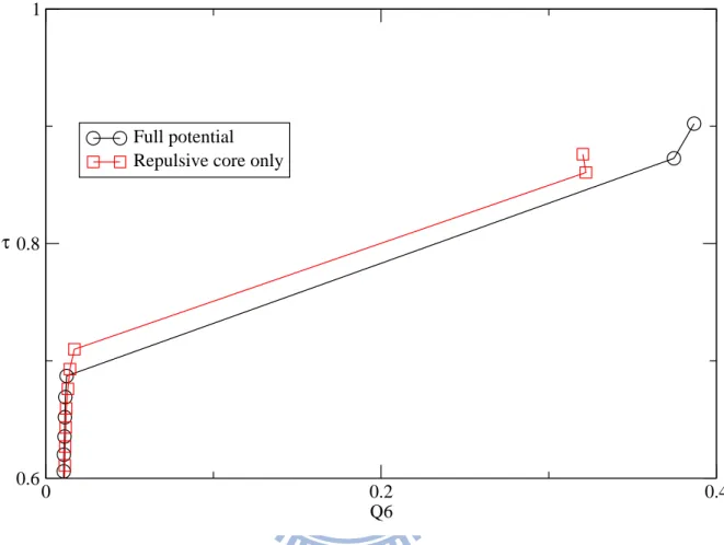
4-2-3 Order map

Fig. 24 shows that the order map of the repulsive core only is almost a straight line because it does not turn to a solid state. But, the order map of the full potential jumps into the top-right part of the figure as the structures

changes to a solid.

We put the order maps of different processes together in Fig. 25 and

compare the g(r) of the corresponding solid states in Fig. 26, which show that different processes are resulted into different solids.

4-2-4 Clusters of Full potential

liquid Ga to -phase Ga, the first peak in g(r) and the cluster numbers grow. But, the temperature effect is very small.

4-2-5 Clusters of Repulsive core only

We consider the distribution of the isolated particles for the two potential models. For Fig. 30 in the liquid state, the isolate-particle number of the full potential is higher than that of the repulsive core only. According to Ref[1], the high-q-side shoulder in S(q) of Ga maybe caused by many “1201 cluster”. If the number of the “1201 clusters” increases, the bond length between 0.89 and 1.1 will also increase. We compare the cluster number with the cutoff at

min

r =0.89 and r_min=1.1. In Fig. 31, the number of different between r_min=0.89

and r_min=1.1 for the full potential indeed grows, for the repulsive core only,

the number difference is almost constant. From S(q) of the full potential case, the high-q shoulder grows up, but for the repulsive core only, S(q) does not have the shoulder, this agrees with Ref[1] that the high-q shoulder is cause by many “1201 clusters”. From g(r) and S(q) of both the full potential and the repulsive core only, we can see that the main reason that causes the system turning into solids in the temperature-quench process should be Friedel oscillations of the potential, so that the repulsive core only, the system does not turn to solids in the quenching process.

Chapter 5

Conclusions

According to the results of our simulations, phase transition can be easily observed with the translational order parameter and the orientational order parameter that we use to describe structure order. Different potentials and different processes in simulations produce different paths in order map. So, we can distinguish different conditions that we use in simulation. Friedel oscillations cause high-density liquid systems with structures less order, but give positive effects on structure order for the system in solid states. The main cause for the high-density solids is the repulsive core of the potential, but the quenched solid is mainly caused by Friedel oscillations of the potential. Our results agree with Ref[1], that “1201 clusters” are the major physical reason for causing the high-q shoulder in S(q).

Reference

[1] S.F. Tsay, S. Wang, Phys. Rev. B 50 108 (1994)

[2] K. H. Tsai, T. M. Wu, and S. F. Tsay, J. Chem. Phys. 132,

034502 (2010)

[3] A.B. de Oliveria, P. A. Netz, J. Chem. Phys. 125, 124505

(2006)

[4] J.R. Errington and P.G. Denedetti, J. Chem. Phys. 118, 2256

(2003)

[5] 黃盈靜，「在 LJ 2n-n 系統內結構次序之量化」，國立交通大

學，碩士論文，民國

97 年。

[6] S. F. Tsay, Phys. Rev. B 50, 103 (1994)

[7] K. H. Tsai and T. M. Wu, J. Chem. Phys. 129, 024503 (2008)

[8] K. H. Tsai, T. M. Wu, S. F. Tsay, and T. J. Yang, J. Phys.

Condens. Matter, 19, 205141 (2007)

[9] M. P. Alen and D. J. Tyndesly, Computer Simulation of Liquids

(Clarendon, Oxford, 1987)

Fig. 6 Variation of translational order parameter with density at T=323K 0 1 2 3 4 ρ 0 0.2 0.4 0.6 0.8 1 τ Full potential Repulsive core only

Fig. 7 Variation of orientational order parameter with density at T=323K 1.5 2 2.5 3 3.5 4 4.5 ρ 0 0.2 0.4 Q6 Full potential Repulsive core only

Fig. 8(a) Static structure factor S(q) of full potential at T=323K

Fig. 8(b) Static structure factor S(q) of repulsive core only at T=323K

20 30 40 50 60 q (nm^-1) 0.5 1 1.5 2 2.5 3 S(q) ρ 3.305 ρ 3.588 ρ 3.87 20 30 40 50 60 q (nm^-1) 0.5 1 1.5 2 2.5 3 3.5 S(q) ρ 3.305 ρ 3.588 ρ 3.87

Fig. 9 Order maps of full potential(circles) and repulsive core only(squares) at T=323K 0 0.2 0.4 Q6 0.6 0.8 1 τ Full potential Repulsive core only

Fig.10 (a) Fig. 10 (e)

Fig.10 Cluster distributions of the full potential with Kc=0.5 and the cutoff of

the bond length atr_min=0.89

0 50 100 150 200 Cluster Size 1e-06 0.0001 0.01 1 % of Cluster Number 3.305 3.21 3.11614 3.02171 0 20 40 60 80 Cluster Size 1e-06 0.0001 0.01 1 % of Cluster Number 2.92728 2.83285 2.73842 2.644 0 10 20 30 40 50 Cluster Size 1e-06 0.0001 0.01 1 % of Cluster Number 2.54957 2.45514 2.36071 2.266285 0 5 10 15 20 25 30 35 Cluster Size 1e-06 0.0001 0.01 1 % of Cluster Number 2.171857 2.0774 1.983 1.8885 E E E 0 2 4 6 Cluster Size 1e-06 0.0001 0.01 1 % of Cluster Number 0.47214 0.37771 0.28328 0.18885 0.094428 E E E E E E 0 2 4 6 8 10 Cluster Size 1e-06 0.0001 0.01 1 % of Cluster Number 0.944285 0.84985 0.755428 0.661 0.56657 E E E E E E E E 0 5 10 15 Cluster Size 1e-06 0.0001 0.01 1 % of Cluster Number 1.41642 1.322 1.22757 1.13314 1.0387 E 0 5 10 15 20 25 Cluster Size 1e-06 0.0001 0.01 1 % of Cluster Number 1.79414 1.69971 1.60528 1.51085

Fig. 11 (a) Fig. 11 (d) Fig. 11 (g)

Fig. 11 (b) Fig. 11 (e) Fig. 11 (h)

Fig. 11 (c) Fig. 11 (f) Fig. 11 (i)

Fig. 11 Cluster distributions of the full potential with Kc=0.5 and the cutoff of

the bond length atr_min=1.1

0 50 100 150 Cluster Size 1e-06 0.0001 0.01 1 % of Cluster Number 3.305 3.21 3.11614 0 50 100 150 Cluster Size 1e-06 0.0001 0.01 1 % of Cluster Number 3.02171 2.92728 2.83285 0 50 100 150 Cluster Size 1e-06 0.0001 0.01 1 % of Cluster Number 2.73842 2.644 2.54957 0 50 100 150 200 Cluster Size 1e-06 0.0001 0.01 1 % of Cluster Number 2.45514 2.36071 2.266285 0 50 100 150 200 Cluster Size 1e-06 0.0001 0.01 1 % of Cluster Number 2.171857 2.0774 1.983 0 50 100 150 Cluster Size 1e-06 0.0001 0.01 1 % of Cluster Number 1.8885 1.79414 1.69971 E E E E E 0 5 10 15 Cluster Size 1e-06 0.0001 0.01 1 % of Cluster Number 0.56657 0.47214 0.37771 0.28328 0.18885 0.094428 E E E E E E E E E E E E E E 0 10 20 30 40 Cluster Size 1e-06 0.0001 0.01 1 % of Cluster Number 1.13314 1.0387 0.944285 0.84985 0.755428 0.661 E E E E E E E_E E_E E_E EE_E EE EE EEE EE_EE E_EE EE EEEE EEEE EEE EEE E E 0 50 100 Cluster Size 1e-06 0.0001 0.01 1 % of Cluster Number 1.60528 1.51085 1.41642 1.322 1.22757 E

Fig. 12 (a) Fig. 12 (e)

Fig. 12 (b) Fig. 12 (f) Fig. 12 (c) Fig. 12 (g) Fig. 12 (d) Fig. 12 (h)

Fig. 12 Cluster distributions of the full potential with Kc=0.5 and the cutoff of

the bond length atr_min=1.3

0 100 200 300 400 500 Cluster Size 1e-06 0.0001 0.01 1 % of Cluster Number 3.305 3.21 3.11614 3.02171 E E E E E E EE_EE EE_EEE EEE EEEE EEEE_EEE EEEE EEEEE EEEEEE EEEE EEEE_EEE EEEEE EEE EEEEEE E EE E E E E E E E E E E EE EEE E EE E E 0 50 100 150 Cluster Size 1e-06 0.0001 0.01 1 % of Cluster Number 2.92728 2.83285 2.73842 2.644 2.54957 E 0 50 100 150 Cluster Size 1e-06 0.0001 0.01 1 % of Cluster Number 2.45514 2.36071 2.266285 2.171857 0 50 100 150 Cluster Size 1e-06 0.0001 0.01 1 % of Cluster Number 2.0774 1.983 1.8885 1.79414 E E E E E E 0 5 10 15 20 Cluster Size 1e-06 0.0001 0.01 1 % of Cluster Number 0.47214 0.37771 0.28328 0.18885 0.094428 E E E E E E E E E E E E E E E E E E E 0 10 20 30 40 50 60 Cluster Size 1e-06 0.0001 0.01 1 % of Cluster Number 0.944285 0.84985 0.755428 0.661 0.56657 E 0 50 100 150 Cluster Size 1e-06 0.0001 0.01 1 % of Cluster Number 1.322 1.22757 1.13314 1.0387 0 50 100 150 200 Cluster Size 1e-06 0.0001 0.01 1 % of Cluster Number 1.69971 1.60528 1.51085 1.41642

Fig. 13 (a) Fig. 13 (e)

Fig. 13 (b) Fig. 13 (f) Fig. 13 (c) Fig. 13 (g) Fig. 13 (d) Fig. 13 (h)

Fig. 13 Cluster distributions of the full potential with Kc=0.5 and the cutoff of

the bond length atr_min=1.5

1 10 100 1000 10000 Cluster Size 1e-06 0.0001 0.01 1 % of Cluster Number 3.305 3.21 3.11614 3.02171 1 10 100 1000 Cluster Size 1e-06 0.0001 0.01 1 % of Cluster Number 2.92728 2.83285 2.73842 2.644 1 10 100 1000 Cluster Size 1e-06 0.0001 0.01 1 % of Cluster Number 2.54957 2.45514 2.36071 2.266285 0 100 200 300 400 Cluster Size 1e-06 0.0001 0.01 1 % of Cluster Number 2.171857 2.0774 1.983 1.8885 E E E E E E E 0 5 10 15 20 25 30 Cluster Size 1e-06 0.0001 0.01 1 % of Cluster Number 0.47214 0.37771 0.28328 0.18885 0.094428 E E E E E E E E E E E E E E E E E E EEE E EE E 0 20 40 60 80 Cluster Size 1e-06 0.0001 0.01 1 % of Cluster Number 0.944285 0.84985 0.755428 0.661 0.56657 E E E E E E E_E E EE EE_EE EE_EE EEE EEE_EE EEEE EEE EEEE EEE EEEE EEEEE E EEEE E EEE E E E EE EE E E E EE E 0 50 100 150 Cluster Size 1e-06 0.0001 0.01 1 % of Cluster Number 1.41642 1.322 1.22757 1.13314 1.0387 E 0 50 100 150 Cluster Size 1e-06 0.0001 0.01 1 % of Cluster Number 1.79414 1.69971 1.60528 1.51085

Fig. 14 (a) Fig. 14 (e)

Fig. 14 (b) Fig. 14 (f)

Fig. 14 (c) Fig. 14 (g)

Fig. 14 (d)

Fig. 14 Cluster distributions of the full potential with Kc=0.5 and the cutoff of

the bond length atr_min=1.76

1 10 100 1000 10000 Cluster Size 1e-06 0.0001 0.01 1 % of Cluster Number 3.305 3.21 3.11614 3.02171 1 10 100 1000 Cluster Size 1e-06 0.0001 0.01 1 % of Cluster Number 2.92728 2.83285 2.73842 2.644 E E E E E E E E E E E E E E E E E E E E E EE_EE E E E E E E E E E EEE E E E E E E E E E E E E E E E EE EEEEEEEE E E E EE E E E E E EEE E E E E E E E E E E E E E E E E E E E E E EE E E E E E E E E E E E EEEEEE_EEEEEEEEEEEEEE E E E E E E E EEE E E E E E E E E E E E EEEE E E E E E E E E E EEEEEEEEEEEEEEEEEEEEEEEEEEEEE E E E E E E E E E E E E EEEEEEEEEEEEEEEEEEEEEEE_EEE_EEEEEEEEEEEEEEEEEEEEEEE_EEEEEE_EEEEEEEEEE_EEEEE_E E E E E E E E E E E_E E E E E E E E E E E E E EEE E E E E E E E E E E EEE_EEEEE E E E E E E_E E E E E E E E E E E E E E E E E E E E E E E E E E E E E EE E E E E E E 0 500 1000 1500 2000 2500 3000 Cluster Size 1e-06 0.0001 0.01 1 % of Cluster Number 2.54957 2.45514 2.36071 2.266285 2.171857 E E E E E E E E E 0 10 20 30 40 Cluster Size 1e-06 0.0001 0.01 1 % of Cluster Number 0.56657 0.47214 0.37771 0.28328 0.18885 0.094428 E E E E E E E E E E E E E_E E E_E E E EEE E_E E EE_E EEEE E EEEE E 0 50 100 Cluster Size 1e-06 0.0001 0.01 1 % of Cluster Number 1.13314 1.0387 0.944285 0.84985 0.755428 0.661 E E E E E E E_E E E EEEEEEEEEEEEEEEEEEEEEEEEEEEEEEEEEEEEEE_EEEEEEEEEEEEEEE_E EEEEEE_EE EEEEEEE_EEE E EEEEEEEE EE_EEEEE E EEE E E E E E E E E E E E E E E E E E E E EE E E EE E E E EEEEEEE E 0 200 400 600 800 Cluster Size 1e-06 0.0001 0.01 1 % of Cluster Number 1.60528 1.51085 1.41642 1.322 1.22757 E E E E E E E_E E E E E E E EEEEEEEEEEEEEEEEEEEEEEEEEEEEEEEEEEEEEEEEEEEEEEEEEEEEEEEEEEEE_EEEEEEEEEEEEEEEEEEEEEEEEEEEEEEEE_EEEEE E E E E E E EEEEEEEEEEEEEEEEEEEEEEEE E E_E E E E E E E E EEEEEE E E E E E E E E E E E EEEEEE E E EEEEEEEEE E E E E E E E E EEE_EE E E E E EE_EEEEEEE E E E E E E E E EEEEEEEEEEEEEEEEE EEEEEEEEEEE E E E E E E E E E E E E E E E EEEE_E E E E E E E E E E E E E EE E E E E E E E EE_EEEEEEEEEEEEEEEE E E E E E E E EEEE_E E E E E EEEE E E E E E E E E E E E E E E_EEEEEE E E EEEEE E E E EEEEEEE E E E E E E E E E E EE E E E E E E E EEEEEEEEEEE E E E E E E EE_EEE E E E E E E E E E E E E EEEEEEEE_E EEEEEEEE EEE E E E E E E EEEEEEE E EEEEEEEEEEEEEEEE E E E E E E E E E E E E E E E E E E EE E E E E E E E E E E E E E E E EEEE E E E E E EEEEEE E E E E E E E E E E E EEEEEEEEEEEEEEEEEE E E E E E E E E EEEEE E E E EE_E E E E E E E EE E E E E E E EE_EEEEEEEEEEEEEEEEEEEEEEEEEEEEEEEEEEE_EE_EEEEEEEEEEEEE EEEEEEEEEEEE E E E E E EE_EEEEEEEEEEEEE_EEEEEEEEEEEEEEEEEEEEEEEEEEEE_EEEE_EEEEEEEE_EEEEEEEEEEEEEEEEEEEEEEEEEEEEE E EEEEEEEEEEEEEEEEEEEEEEEEEEEEEEEEEEEEEEEEEEEEEEEEEEEEEE_EE_EEEEEEEE E E E E E EE_EEEEEEEEEEEEEEEEEE_EE E E E EEE E E E E E E EEEEEEEE E EEEEEEEEEE E E E E E E E EEEE_EE E E E_EEEE E E E E E E E E E E E E E E E E E E E E E EE E E E E E E EEEE E E E E E EEEE E E E E E E E E E E E E EE E E E E E E E E E E E E E E E E E E E E E E E E EE E EEEEEEEE 0 500 1000 1500 2000 Cluster Size 1e-06 0.0001 0.01 1 % of Cluster Number 2.0774 1.983 1.8885 1.79414 1.69971 E

Fig. 15 Density variation of the isolated-particle number for the full potential

with the cutoff distance r_min=0.89, 1.1, 1.3, 1.5 and 1.76

E E E E E E E E E E E E E E E E E E E E E E E E E E E E E _{E E E E E E} 0 1 2 3 Density 0 0.2 0.4 0.6 0.8 1 % of isolate particle Rmin 0.89 Rmin 1.1 Rmin 1.3 Rmin 1.5 Rmin 1.76 E

Fig. 16 (a) Fig. 16 (d)

Fig. 16 (b) Fig. 16 (e)

Fig. 16 (c) Fig. 16 (f)

Fig. 16 The g(r) function of the full potential at T=323K and different density

0 1 2 3 4 5 r* 0 1 2 3 4 5 6 g(r) 3.682714 3.777142 3.871571 4.06042 4.154857 0 1 2 r* 0 1 2 3 g(r) 3.305 3.21 3.11614 3.02171 2.92728 2.83285 0 1 2 r* 0 0.5 1 1.5 2 2.5 g(r) 2.73842 2.644 2.54957 2.45514 2.36071 2.266285 2.171857 2.0774 1.983 0 1 2 r* 0 0.5 1 1.5 g(r) 0.37771 0.28328 0.18885 0.094428 0 1 2 3 r* 0 0.5 1 1.5 2 g(r) 0.944285 0.84985 0.755428 0.661 0.56657 0.47214 0 1 2 3 r* 0 0.5 1 1.5 2 g(r) 1.8885 1.79414 1.69971 1.60528 1.51085 1.41642 1.322 1.22757 1.13314 1.0387

Fig. 17 Cluster distributions of the repulsive core only with Kc=0.5 and the

cutoff of the bond length atr_min=0.89

E E E E E E_E E_E E_EE E_EEE E_EEEE EEEEEEEEEEEEE_E EEEEEEEE_EE_EE_EE_EE EEE_EEEEEEE_EEE_EE_EE_EEEE_EE_EE EEEEEEEEEEEEE_EEEEEE_EE_EEE EEEE_EEEE_EEE EE E E E_E EEEEEE_EEEEEEE_EE EE E E E_EEE EE EE E E E E E E_E EEE E_E E E EEEE E E_E EEE_EE EE_EE E EEEE_E E E_EEEE_EEEEEE_E E E EEEE E E E EE_E EEEE E E_E E EEEEE_EEE_EE_EE_E E E_E E E_E E E EEE E E E EEEE E EE EEE E EE E EE E_E E E E E E EE E EEE_EE E E E EEE E E E E EEE E E EEEE E E E E E E_E E EEEEE EE EE E E E EEEE E E E E E EE E E E E E E E E EE EEE E EEE EEE 0 50 100 150 200 250 300 350 Cluster size 1e-06 1e-05 0.0001 0.001 0.01 0.1 1

Cluster number/ total particle number

ρ 0.85 ρ 1.51 ρ 2.08 ρ 2.74 ρ 3.305 ρ 3.68 E

Fig. 18 (a) Fig. 18 (e)

Fig. 18 (b) Fig. 18 (f)

Fig. 18 (c) Fig. 18 (g)

Fig. 18 (d)

Fig. 18 Cluster distributions of the repulsive core only with Kc=0.5 and the

cutoff of the bond length atr_min=1.1

0 50 100 150 200 250 Cluster Size 1e-06 1e-05 0.0001 0.001 0.01 0.1 1 % of Cluster number 3.305 3.21 3.11614 3.02171 E E E E E E EE_EE EEE_EEE EEEE_EEEE EEEEE EEEEE_EEE EEEE EEEEEE_EEEEE EEEEE EEEE EEEEEEEE E E EE_E E E E EE E E E E E E E E EE E E EEEEE EEEEEEEEE E

0 50 100 150 200 Cluster Size 1e-06 1e-05 0.0001 0.001 0.01 0.1 1 % of Cluster number 2.92728 2.83285 2.73842 2.644 E 2.54957 E E E E E E EE_EE EEE_EEE EEE EEEE_EEE EEEEEEE EEEEE_EEE EEEE EEEEE_EEE EEEEEEEEE E EE E EE E E E E E EEE_EE_E E EE EE E E E EEE _E 0 50 100 150 200 Cluster Size 1e-06 0.0001 0.01 1 % of Cluster number 2.45514 2.36071 2.266285 2.171857 E 2.0774 E E E E E E E 0 2 4 6 8 10 12 14 16 18 20 22 24 26 28 30 Cluster Size 1e-06 1e-05 0.0001 0.001 0.01 0.1 1 % of Cluster Size 0.56657 0.47214 0.37771 0.28328 E 0.18885 0.094428 E E E E E E E E E E E E E E E E E E 0 10 20 30 40 50 Cluster Size 1e-06 1e-05 0.0001 0.001 0.01 0.1 1 % of Cluster number 1.13314 1.0387 0.944285 0.84985 E 0.755428 0.661 E E E E E E E E E_E E_E EE EE EE EE EE EEE EE EE_EE EEE_E EEEEE EE EE EE EE E 0 20 40 60 80 100 Cluster Size 1e-06 0.0001 0.01 1 % of Cluster number 1.60528 1.51085 1.41642 1.322 E 1.22757 E E E E E E EE EE EEE EEE_EEE EEE_EEE EEE_EEE EEE_EEEE EEE_EEE EEEE EEEEE EEEEEE EEEEE E E EE EEE E EE E EE E E EE 0 50 100 150 Cluster Size 1e-06 1e-05 0.0001 0.001 0.01 0.1 1 % of Cluster number 1.983 1.8885 1.79414 1.69971 E

Fig. 19 (a) Fig. 19 (e)

Fig. 19 (b) Fig. 19 (f) Fig. 19 (c) Fig. 19 (g) Fig. 19 (d) Fig. 19 (h)

Fig. 19 The g(r) function of the repulsive core only at T=323K and different

0 0.5 1 1.5 2 2.5 r* 0 1 2 3 g(r) 3.305 3.21 3.11614 3.02171 2.92728 0 0.5 1 1.5 2 2.5 r* 0 0.5 1 1.5 2 2.5 g(r) 2.83285 2.73842 2.644 2.54957 2.45514 0 0.5 1 1.5 2 2.5 r* 0 0.5 1 1.5 2 2.5 g(r) 2.36071 2.266285 2.171857 2.0774 1.983 0 1 2 r* 0 0.5 1 1.5 g(r) 0.47214 0.37771 0.28328 0.18885 0.094428 1 2 3 r* 0 0.5 1 1.5 2 g(r) 0.944285 0.84985 0.755428 0.661 0.56657 1 2 3 r* 0 0.5 1 1.5 2 g(r) 1.41642 1.322 1.22757 1.13314 1.0387 0 1 2 r* 0 0.5 1 1.5 2 g(r) 1.8885 1.79414 1.69971 1.60528 1.51085 0 1 2 r(σ) 0 1 2 3 4 5 g(r) ρ=3.588 ρ=3.777 ρ=3.872 ρ=4.06

Fig. 20(a)

Fig. 20(b)

Fig. 20 Distribution of the isolated particles in the full potential (circles) and

the repulsive core only (squares) with r_min=0.89(a) and r_min=1.1(b)

0 1 2 3 4 ρ 0 0.2 0.4 0.6 0.8 1

isolate particle number / total particle number

Full potential Repulsive core only

0 1 2 3 4 ρ 0 0.2 0.4 0.6 0.8 1

isolate particle number / total particle number

Full potential Repulsive core only

Fig. 21 Temperature variation of the translational order parameter at ρ =3.305 for the models of the full potential (circles) and the repulsive core only (squares)

120 140 160 180 200 220 240 260 280 300 320 Temperature (K) 0.5 0.6 0.7 0.8 0.9 1 τ Full potential Repulsive core only

Fig. 22 Temperature variation of the orientational order parameter atρ=3.305 for the models of full potential (circles) and the repulsive core only (squares) 120 140 160 180 200 220 240 260 280 300 320 Temperature (K) 0 0.2 0.4 Q6 Full potential Repulsive core only

Fig. 23(a)

Fig. 23(b)

Fig. 23 Static structure factors S(q) of the full potential (a) and the repulsive core only (b) at ρ=3.305 20 30 40 50 60 q (nm^-1) 0.5 1 1.5 2 2.5 S(q) 323K 253K 203K 153K 20 30 40 50 60 q (nm^-1) 0.5 1 1.5 2 2.5 S(q) 323K 253K 203K 153K

Fig. 24 Order maps for the models of the full potential (circles) and the repulsive core only (squares) at ρ=3.305 and several temperatures

0 0.1 0.2 0.3 0.4 Q6 0.6 0.7 0.8 0.9 τ Full potential Repulsive core only

Fig. 25 Comparison for the order map of the temperature and density variations for the models of the full potential and the repulsive core only

0.1 0.2 0.3 0.4 Q6 0.6 0.7 0.8 0.9 τ

density variation Full potential density variation Repulsive core only temperature variation Full potential temperature variation Repulsive core only

Fig. 26 Comparison for the radial distribution functions g(r) of the solids obtained by different simulation process

0 1 2 3 r(σ) 0 1 2 3 4 5 g(r)

density variation Full potential density variation Repulsive core only temperature variation Full potential temperature variation Repulsive core only

Fig. 27(a)

Fig. 27(b)

Fig. 27 The cluster distributions of the full potential at ρ=3.305 and three

temperatures with the cutoff r =0.89 (a) and r =1.1 (b)

0 50 100 150 Cluster size 1e-06 1e-05 0.0001 0.001 0.01 0.1 1

Cluster number/total particle number

313K 243K 153K 0 50 100 150 200 Cluster size 1e-06 1e-05 0.0001 0.001 0.01 0.1 1

Cluster number/ total particle number

313K 243K 153K

Fig. 28(a)

Fig. 28(b)

Fig. 28 The cluster distributions of the repulsive core only at ρ=3.305 and

three temperatures with the cutoff r_min=0.89 (a) and r_min=1.1 (b)

0 50 100 150 200 250 300 Cluster size 1e-06 1e-05 0.0001 0.001 0.01 0.1 1

Cluster number/ total particle number

313K 243K 153K 0 50 100 150 200 Cluster size 1e-06 1e-05 0.0001 0.001 0.01 0.1 1

Cluster number/ total particle number

313K 243K 153K

Fig. 29 The g(r) function of the full-potential model atρ=3.305 and T=313k, 283K, 173K, 153K and 103K 0.5 1 1.5 2 r* 0 1 2 3 4 5 g(r) 313K 283K 173K 153K 103K

Fig. 30(a)

Fig. 30(b)

Fig. 30 Temperature variation of the isolated-particle distribution for the full potential (circles) and the repulsive core only (squares) with the cutoff at

min

r =0.89 (a) and r_min=1.1 (b)

120 140 160 180 200 220 240 260 280 300 320 Temperature (K) 0 0.1 0.2 0.3 0.4 0.5

isolate particle number / total particle number

Full potential Repulsive core only

120 140 160 180 200 220 240 260 280 300 320 Temperature (K) 0 0.1 0.2 0.3 0.4 0.5

isolate particle number / total particle number

Full potential Repulsive core only

Fig. 31 The difference between the isolated-particle distribution atrmin=0.89

and r_min=1.1 for the models of the full potential (circles) and the repulsive

core only (squares)

160 180 200 220 240 260 280 300 320 Temperature (K) 0 0.01 0.02 0.03 0.04 0.05 0.06 0.07

isolate particle number difference

Full potential Repulsive core only