在H.264/先進視訊編碼壓縮領域中做鏡頭變化的偵測

國

立

交

通

大

學

資訊科學與工程研究所

碩

士

論

文

在 H.264/先進視訊編碼壓縮專業領域中做鏡

頭變換的偵測

Shot change detection in H.264/AVC compression domain

研 究 生：黃重輔

指導教授：蔡文錦 教授

在 H.264/先進視訊編碼壓縮領域中做鏡頭變化的偵測

Shot change detection in H.264/AVC compression domain

研 究 生：黃重輔 Student：Chung-Fu Huang

指導教授：蔡文錦 Advisor：Wen-Jiin Tsai

國 立 交 通 大 學

資 訊 科 學 與 工 程 研 究 所

碩 士 論 文

A Thesis

Submitted to Institute of Computer Science and Engineering College of Computer Science

National Chiao Tung University in partial Fulfillment of the Requirements

for the Degree of Master

in

Computer Science November 2008

Hsinchu, Taiwan, Republic of China

在 H.264/先進視訊編碼壓縮領域中做鏡頭變化的偵測

學生：黃重輔 ………指導教授：蔡文錦

國立交通大學資訊科學與工程研究所碩士班

摘要

鏡頭變換偵測演算法在自動化的視訊內容分析、索引、以及擷取方面為一基礎 的步驟。鏡頭變換的偵測可以應用在很多種視訊技術領域，例如: 視訊編碼解碼的 品質與效能以及轉換編碼的的準備等。這篇論文根據 intra macroblock 預測模式 之中的邊的方向性相似度以及 intra 和 inter macroblock 個數的比例提出了一個 新的 H.264/AVC 壓縮頻域上鏡頭變換偵測的方法。這篇提出的鏡頭變換偵測演算法 包含平緩的鏡頭偵測及切割鏡頭變換的偵測。在平緩鏡頭偵測部份，我們提出了一 個褪去鏡頭變換偵測演算法，利用 intra macroblock 個數的比例以及 P_SKIP 模式 的 macroblock 個數比例去決定出起始點和終止點。接著，邊的方向性相似度則是 利用來判斷目前所偵測到這張宏塊是否包含在褪去鏡頭之中。在切割鏡頭變換的偵 測中，我們使用 P-MB 和 B-MB 個數的比例去偵測出切割鏡頭變換宏塊的候選者，接 者利用我們所提出的邊的方向性相似度去判斷這個候選者是否為一個切割鏡頭變

換的宏塊。 實驗結果顯示出我們提出的演算法藉由正確度與精確度頻估對於不同種類的 視訊具有高度的正確性即使在變動性的位元比率中。我們提出的邊的方向性相似度 方法也可以加強鏡頭變換偵測演算法以及達到令人滿意的效果。 關鍵字：視訊內容分析，索引，以及擷取，鏡頭變換偵測，視訊分析，平緩鏡頭偵 測，切割鏡頭偵測，壓縮頻域，H.264/AVC

Shot change detection in H.264/AVC compression domain

Student: Chung-Fu Huang Dvisor: Wen-Jiin Tsai

Department of Computer Science National Chiao-Tung University

ABSTRACT

Shot change detection algorithm is a fundamental step in automatic video content analysis, indexing, and retrieval. Shot change detection can apply to many kinds of video technology fields, for example, video codec compression quality and performance and transcode preparation…etc. This thesis proposed a new shot change detection method using edge direction similarity based on intra macroblcok prediction mode and the ratio of intra to inter macroblocks in H.264/AVC compression domain. The proposed shot change detection algorithm includes gradual shot change and cut shot change detection. In gradual shot change detection, we proposed a fade shot change detection algorithm, using intra macroblock ratio and P_SKIP macroblock ratio to decide start point and end point. Then edge direction similarity is used to judge if current detected frame is included in the gradual shot or not. In cut shot change detection, we use P-MB and B-MB ratio to detect candidate cut change frame, and then use proposed edge direction similarity to judge the candidate frame is a cut change or not.

The experimental result shows that our proposed algorithm has a high accuracy in terms of recall and precision for a variety of video streams even they are variable bit rates. Our proposed edge direction similarity approach also can enhance shot change detection algorithms and achieve satisfactory performance.

Keyword: Video content analysis, indexing, and retrieval, shot detection, video analysis, gradual shot detection, cut shot detection, compression domain, H.264/AVC.

Contents

摘要 ... i

ABSTRACT ... iii

Chapter 1 Introduction ... 1

Chapter 2 Related Works ... 4

-2.1 Shot type identification methods ... - 4 -

2.1.1 Gradual shot transition identification... - 4 -

2.1.2 Cut shot change identification ... - 6 -

2.2 Shot detection methods ... - 8 -

Chapter 3 Proposed Fades And Cut ... 12

Detection Algorithm ... 12

-3.1 Fade Out Shot Transition Detection Algorithm ... - 12 -

3.2 The flowchart overview of fade out shot transition detection algorithm: . - 28 - 3.3 Fade In Shot Transition Detection Algorithm ... - 29 -

3.3 Cut Shot Change Detection Algorithm ... - 32 -

Chapter 4 Experimental Results ... 36

-4.1 Performance Evaluation Criteria ... - 36 -

4.2 Test Video Sequence and Evaluation Enviroments ... - 37 -

4.3 Performance Comparison with Different Fades Detection Methods ... - 39 -

4.4 Performance Comparison with Different Shot Change Detection Methods- 41 - 4.5 Performance Comparison between Different Shot Detection Methods and our enhanced Shot change Detection Methods ... - 43 -

4.6 Performance Evaluation for the Video Sequences with Different Bit-Rates- 46 -

Chapter 5. Conclusion and Future Works ... 47

-List of Figures

FIGURE 1:GRADUAL SHOT TRANSITION (A)SMOOTH THE GRADUAL AND DIMINISH PEAKS (B) ... -5

-FIGURE 2:THE 15 PARTITION SIZES OF THE MACROBLOCKS HISTOGRAM, GET FROM REF[15] ... -6

-FIGURE 3:THE EDGE REGION CLASSIFICATION ... -10

-FIGURE 4:THE EXPERIMENTAL RESULTS OF THE START POINT OF IMDR VALUE FOR VIDEO SEQUENCES “JOHNRAMBO”,“RESCUE_DAWN”, AND “CASINO_ROYALE” RESPECTIVELY. ... -14

-FIGURE 5: CASE 1 IS DETECTED BY USING IMDR AND IMR FEATURE. ... -16

-FIGURE 6:CASE 2 IS DETECTED BY USING IMDR AND IMR FEATURE. ... -17

-FIGURE 7(A):THE FLOWCHART OF CASE 1 DETECTION ALGORITHM. ... -17

-FIGURE 8:(A),(B)THE EXPERIMENTAL RESULTS OF IMDR RATIO AND IMR RATION DURING FADE OUT SHOT TRANSITIONS. ... -19

-FIGURE 9:(A)THE NINE DIFFERENT EDGE DIRECTION SLOPES FOR INTRA4X4 PREDICTION MODES.(B)THE NINE DIFFERENT INTRA4X4 PREDICTION MODES... -21

-FIGURE 10:THE EXAMPLES FOR W_VALUE SETTING ... -22

-FIGURE 11:THE EXAMPLES FOR W_VALUE SETTING ... -23

-FIGURE 12:THE EXPERIMENTAL RESULTS OF THE ASWV ... -25

-FIGURE 13:THE EXPERIMENTAL RESULTS OF THE ASWV ... -25

-FIGURE 14:THE COMPLETE FLOW CHART OF FADE OUT SHOT TRANSITION DETECTION ALGORITHM .... -28

-FIGURE 15:THE EXPERIMENTAL RESULTS OF THE START POINT OF IMDR VALUE FOR VIDEO SEQUENCES “JOHNRAMBO”,“RESCUE_DAWN”, AND “CASINO_ROYALE” RESPECTIVELY. ... -30

-FIGURE 16:THE IMDRI-1,I, IMDRI-2,I, AND IMDRI-3,I. ... -30

-FIGURE 17:THE EXPERIMENTAL RESULTS OF IMDRI-1,I,IMDRI-2,I-1, AND IMDRI-3,I-2VALUES. ... -32

-FIGURE 18:THE EXPERIMENTAL RESULTS OF THE PHD THRESHOLD. ... -33

-FIGURE 19:THE EXPERIMENTAL RESULTS OF THE ASWV ... -34

-List of Tables

TABLE 1:AVERAGE PERCENTAGE OF MBS WHICH ARE CODED IN INTER OR INTRAMODE, GET FROM

REF[12]. ... -8

-TABLE 2:EDGE DIRECTION OF INTRA PREDICTION MODE, GET FROM REF[12] ... -9

-TABLE 3:THE NUMBER OF SHOTS AND THE SHOT TYPES ... -38

-TABLE 4:THE THRESHOLDS SET ... -38

-TABLE 5(A):THE EXPERIMENTAL RESULTS OF PROPOSED FADE OUT/IN DETECTION ALGORITHMS. ... -40

-TABLE 6:(A),(B),(C), AND (D) ARE THE EXPERIMENTAL RESULTS OF SHOT CHANGE ALGORITHMS PROPOSED BY BOHYUN,SASTRE,KLAUS, AND US RESPECTIVELY. ... -43

-TABLE 7:THE EFFECTS OF THE PROPOSED CUT_IPES ALGORITHM.(C) AND (D) ARE THE BAR CHARTS OF RECALL AND PRECISION BY COMPARING WITH DIFFERENT SHOT CHANGE DETECTION ALGORITHM.-45 -TABLE 8:(A),(B)THE EXPERIMENTAL RESULTS OF DIFFERENT VIDEO TEST SEQUENCES UNDER VARIOUS DIFFERENT BIT-RATES. ... -47

-Chapter 1 Introduction

In recent years, due to many rapid improvements in video compression and several areas of computing, the amount of multimedia information has been explosively increased. Searching for the interested video from an immense amount of multimedia streams is not easy. To solve this problem, many researchers worked on parsing video sequences into shots to achieve automatic video content analysis, indexing and browsing, where a shot is defined as a sequence of images captured from one camera [1]. Additionally, shot change detection can also be applied on many kinds of video technology fields such as video compression [9] and transcoding (frame skip etc)…etc.

Generally, there are two different types of transitions between shots:

Cut shot transitions: A cut transition is an abrupt shot change from one frame to

another. A Cut shot transition usually consists of only one frame.

Gradual shot transitions: During a gradual shot transition, the transition of one shot

to another proceeds gradually such as fade shots, dissolve shots, and wipe shots. During a fades shot transition, a shot gradual translates from a solid frame to a blank one or via versa. During a dissolve shot transition, the previous shot fades out gradually while the next shot fades in gradually. The gradual shot transition usually consists of more than one frames.

In general, cut shot is the most common and simplest way to present movement from one shot to another. Those shot change transitions are relatively easy to be detected because the correlations between the succeeding frames at a cut boundary are

the difference between the adjacent two frames are not distinguishable during a gradual shot transition. Gradual shot transitions are usually used at scene boundaries, to accentuate something change in video content. For example, fade shot transitions are often used in films and movie trailers to represent the time elapse, the two fade in/out combinations denotes some kinds of relative mood and pace between shots[10], wipe shot transitions often indicates subtitle changes in video stream, and dissolves shot transitions describes the movie special efficacy and an emotion change. Hence, detecting gradual shot transitions in video streams can be used in semantic based video retrieval, browsing, and analysis and also be contributive to video summarization and video skimming applications.

Previous researched shot detection algorithms can be classified into two groups: Uncompressed domain method and compressed domain methods.

Uncompressed domain method: Approaches utilize information feature directly

from decompressed pixel-domain of video bit stream such as edge direction characteristics[2],object boundaries[3],color histogram[4], and correlation average[5].

Compressed domain method: Approaches utilize extracted clues directly from

compressed video stream such as macroblock type [6], [15], motion vector [7], [16], and DC coefficients [8], [17] .

Uncompressed domain shot change detection is usually computationally demanding and time consuming but obtains better results. Since almost all video streams are stored in compressed format, if uncompressed domain approaches suffer from the need of decoding the compressed bit streams, and, therefore, are time consuming and computational overhead. H.264/AVC is the most recent video compression standard because of its superior compression performance among current international video codec standards. However the most shot change detection methods are not designed

for H.264/AVC and cannot take advantages of its unique encoding techniques such as intra prediction, to achieve a better result. Therefore, a novel algorithm for shot change detection in H.264/AVC compressed domain becomes more important issue.

In this thesis, we expolred the diversity of shots and proposed two different shot change algorithms: Cut shot change detection algorithm and fades shot change detection algorithm. The cut shot change detection algorithm focuses on INTER macroblcok variation between shots and then uses edge direction similarity to enhance detection accuracy. The fades shot change algorithm uses intra and P_SKIP macroblcok features to decide the start point and the end point of a fades shot transition and then uses edge direction similarity to decide whether the current frame is included in fades shot transitions. The experimental results show that our proposed algorithm has much better performance compared with other shot change detection methods. This thesis is organized as follows. Chapter 2 describes various shot change detection methods and their respective conceptions. In chapter 3, the proposed algorithms are presented. Chapter 4 presents some experiment results. Finally, the discussion and future works are drawn in chapter 5.

Chapter 2 Related Works

In chapter 1, several shot change detection algorithm techniques have been introduced. Most of existing methods focused only on single shot change detection but not identified the shot to be a cut shot change or a gradual shot transition. Discriminating a shot to be a cut shot and a gradual shot transition is important. A gradual shot transition includes more than one frames and a cut shot contains only one frame. The evaluations of the cut shot change detection methods and a gradual transition detection methods should be different (that will be discussed in Chapter 4). Chapter 2.1 introduced the previous methods that can identify the type of a shot (Cut shot or Gradual shot transition). Chapter 2.2 introduced the method that only provides shot detection but not identify the shot type.

2.1 Shot type identification methods

2.1.1 Gradual shot transition identification

The gradual shot transition algorithm proposed in [10] is based on smoothing the metric which is defined by percentage of the intra-coded macroblocks and diminishing the peaks by applying a Gaussian filter as illustrated in figure 1.a. Then it made use of two variable thresholds Ta and Tb based on characteristics of proceeding frames. Using the mean and variation of metric for a number of proceeding frames to determine the adaptive threshold Ta. Once the metric of current frame exceeded the threshold Ta, the frame is marked as a start point of a gradual shot transition (the result showed in figure 1.b). And the following frames are inspected by using

)

(i

Δ

threshold Tb to determine whether they belong to the gradual shot transition or not (the result showed in 2.c). The advantages in ref [11] are used simple conceptions to detect gradual transition. However, the computation overheads of Gaussian filter is very huge and the filtered effects are not good to do the threshold setting.

Figure 1: Gradual shot transition (a) Smooth the gradual and diminish peaks (b) Detection of the start point of gradual shot transition (c) The gradual shot transition found by algorithm, get from ref [10].

In [11], there are several steps working on gradual shot transition detection. The first step is to collect candidate frames into a candidate set (CS) based on intra macroblock proportion (IMR). The second step is to group some frames from candidate set CS together to form a gradual shot transition, where the group G, consisting of consecutive candidate frame Ci within a frame-distance , is built according to the following equations:

We defined a symbol |G| which denoted the total number of frames in group G. If and only if the |G| value is between minGopsize and maxGOPsize, setting the group G is a gradual shot transition candidate. The last step is to eliminate false alarms produced by second step. To detect incorrect gradual shot transitions, the last step checks the frame distance between two succeeding gradual transition detected in step 2. If the frame distance is less than or equal to a predefined threshold Thr, the next gradual shot transition is removed. However, this method is not so efficiency in identifying gradual shot transitions from our experimental result. Because the algorithm only used intra macroblck ratio feature which is not good enough for gradual shot detection even through it will remove some false alarms.

2.1.2 Cut shot change identification

In [11], the cut shot change algorithm is proposed by using the relation of P-MBs and B-MBs between the first frame and the second frame in a new cut shot. They used a partition histogram consisting of 15 bins according to the partition sizes of the macroblock-related defined by H.264/AVC standard (showed in Figure 2).

Figure 2: The 15 partition sizes of the macroblocks histogram, get from ref[15]

frame

candidate

ing

correspond

the

of

number

frame

denoted

fn

where

CS

C

j

i

k

C

fn

C

fn

C

C

G

_{i j k k}

()

,

,

1

...

,

)

(

)

(

},

...

{

₁

−

≤

Δ

∀

=

−

∈

=

₊

Specially, the partition histogram difference (PHD) is calculated as the sum of differences of the histogram bins between the current detected ith frame and the

preceding i-1th frame that defined as follow:

In order to enable uniform rating of the different partition types, using a scaling vector of 4x4 blocks. The PHD equation is refined as follow:

, where W is the dynamic weight which specified as the maximum number of 4x4 partitions for the current detected ith frame and preceding i-1th frame, and Sb is the

scaling vector of bth histogram bin. So, when the value of PHD exceeds a predefined

threshold (Thr), the cut shot change is occurred.

bin

histogram

partition

the

is

b

where

b

b

i

H

b

i

H

PHD

15

,

1

1

∑

=

−

−

=

⎟ ⎠ ⎞ ⎜ ⎝ ⎛

b

S

b

b

i

H

b

i

H

W

PHD

∑

=

−

−

=

⎟ ⎠ ⎞ ⎜ ⎝ ⎛

15

1

1

1

2.2 Shot detection methods

The proposed shot change detection algorithm in [12] used the feature that when shot change happened, the majority of macroblocks will be coded in INTRA mode and the histogram of edge direction of intra prediction to detection a shot change. The table 1 shows the average percentage of intra blocks in each predictive frame. Firstly, computing the intra macroblcok percentage of current detected frame and compare to a predefined threshold (Tc) in order to decide whether the frame be a shot

change

candidate.

Table 1: Average percentage of MBs which are coded in INTER or INTRA Mode, get from ref[12].

After that, using edge direction feature to enhance the accuracy of shot change. Intra prediction mode in H.264/AVC is classified into 4 types of 16x16 mode and 9 types of 4x4 mode, the edge direction value of each type is determined by arctan computing (showed in Table 2).

Table 2: Edge direction of INTRA prediction mode, get from ref[12]

When the macroblock is decided as INTRA mode, for each 4x4 subblock of one macroblock has a certain edge direction value. The algorithm computes an average edge direction value of the 8x8 block with the edge direction value of each prediction mode as above mentioned. That is, the edge value of 8x8 block is calculated by the average of the edge direction value of four 4x4 subblocks. Then they defined the edge region of the 8x8 block by the edge direction value.

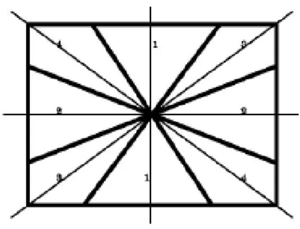
The figure 3 is showed the edge region classification. If the edge direction value of 8x8 block computed between 67.5-degree and 112.5-degree or between 247.5-degree and 292.5-degree, it belongs to edge region 1. The dominate edge direction of the 8x8 block is vertical. Similarly, if the edge direction value of 8x8 block belongs to the region 2, 3, or 4, then the 8x8 blocks have the dominate edge of horizontal, 45-degree orientation, and 135-degree orientation respectively.

Figure 3: The edge region classification

The algorithm used the Edge Histogram Descriptor (EHD) in MPEG-7 represented a local edge distribution in images [13]. Specifically, dividing the frame image into 16 sub-images, the local edge distribution of each sub-image can be represented by EHD histogram. Using the edge region classification as above mentioned, to generate the EHD histogram. Edge direction values in each sub-image can be categorized into five dominate edge types: vertical, horizontal, 45-degree diagonal, 135-degree diagonal and non-edge. Since having 16 sub-images and five different dominate edge types, total 80 histogram bins are required.

In order to detect shot change, the algorithm used the difference value of EHD histogram between candidate frames which is defined as follow equation:

, where EHBi(K) is the ith EHD histogram bin in Kth frame. When the value of EHBD

is larger than a predefined threshold (T), a shot change is detected.

In [14], the shot change detection algorithm proposed by using two basic

∑

=

−

−

=

80 1

)

1

(

)

(

)

(

i i i

K

EHB

K

EHB

K

EHBD

thresholds, one is fixed and another is adaptive, and some auxiliary parameters. These two basic thresholds are all expressed as a percentage of the intra macroblcks of a coded frame. The fixed threshold is used as a reliability measure, and setting a high value to guarantee that the percentage of intra macroblcks of the detected frame exceeded the threshold value is a shot change occurred. To reinforce the shot change detection, the algorithm is used the relation feature of the total number of intra macroblocks between current detected frame and previous frames by means of the adaptive threshold. The adaptive threshold is set depend on the average of intra macroblcoks of the frame encoded since the last INTRA frame. The span parameter S is set to determine which thresholds are active by comparing the current encoded frame number with S value. If the current encoded frame number exceeded the S value, both two basic thresholds detection will be active; Else, only the fixed threshold detection will be active. However, although this algorithm has a good accuracy of recall, the accuracy of precision is very low because it doesn’t have meticulous method to eliminate false alarms generated by the adaptive threshold detection.

Chapter 3 Proposed Fades And Cut

Detection Algorithm

In this section, we’ll introduce our proposed algorithms which include the gradual shot transitions detection algorithms and the cut shot change detection algorithm. For the gradual shot detection, we focus on fade out and fade in detection only. Some of the key features of our proposed method are listed as follow:

1. The proposed method works in the H.264/AVC compressed domain. There is no need of decoding the video bitstreams and hence, it is efficiency.

2. It works effective and robust in various variable bit-rate environments.

3. It is able to identify shot types and precisely recognize boundaries of the fades shot transitions.

3.1 Fade Out Shot Transition Detection Algorithm

There are four steps in the proposed algorithm.

(I) Start point detection: To find out the potential start frame of a fade out shot transition.

(II) Brightness change analysis: To analysis the brightness variations between frames during a fade out shot transition.

(III) Edge direction similarity check: We proposed an intra prediction edge similarity (FADES_IPES) algorithm to check whether a frame is in a fade out shot transition or not.

transition.

(I) Start Point Detection

During the fade out shot transition, a shot gradually disappears and end with a solid color image. In a general fade out transition, there is a brightness variations between the first frame and the second frame. Because of the brightness variations between two adjacent frames during a fade out shot transition, the most macroblocks of frames are encoded in INTRA mode. Therefore, this implies that the difference in the ratio of INTRA macroblocks provides the clue to fine out the start point of a fade out transition. Let IMDR denotes the Intra macroblocks ratio difference (IMDR), which is defined in equation (1) and (2).

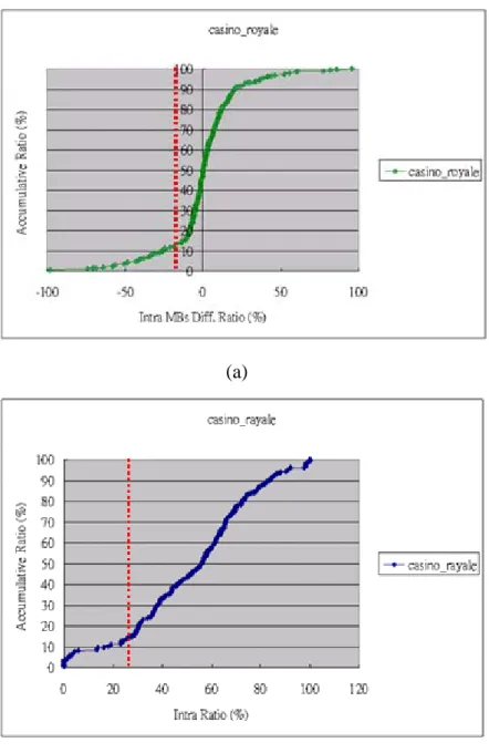
We calculated the IMDR value frame by frame. A frame is a start point candidate of a fade out shot transition if its IMDR value is within a predefined range. In order to decide an appropriate IMDR threshold for start point detection, we collect information from three sequences: “ johnrambo ”, ” rescue_dawn ”, and “ casino_royale ”. For each sequence, we calculate the IMDR values for each start point frame and conduct the start-point ratio for each IMDR value. The start-point ratio of a IMDR value, α,

)

2

(

#

#

−

−

−

−

−

−

−

−

−

−

−

−

=

i

frame

in

MBs

of

i

frame

in

MBs

Intra

of

i

IMR

)

1

(

1

,

1

=

−

−

−

−

−

−

−

−

−

−

−

−

−

−

t

IMR

t

IMR

t

t

IMDR

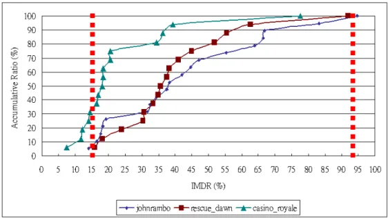
number of start point frames in the sequences. A IMDR value with a higher start-point ratio means that it has the higher probability to correctly detect the start point of a fade out shot transition. The statistical results are shown in figure 4, where it displays the accumulated start-point ratio as a function of IMDR values, ranging from 0 to 100. Therefore, we set the lower bound and upper bound of the IMDR to be 15 and 96 respectively. For a frame with 15<=IMDR<=96, it will be regarded as a potential start point of a fade out transition. The threshold range of IMDR is wide because we do not want to lose the precise position of start point in a fade out transition.

Figure 4: The experimental results of the start point of IMDR value for video sequences “johnrambo”, “rescue_dawn”, and “casino_royale” respectively.

(II) Brightness Change Analysis

Generally, most macroblocks of frames are coded using INTRA mode during a fade out shot transition because of the brightness variations. But in some situations like film shooting skills and video streaming content difference etc, it’s possible there

are not obvious brightness changes between two succeeding frames during the fade out shot transitions. However, across more frames, there are still obvious brightness change and are still in fade-out transition. Hence, we used IMDR and IMR to detect whether or not the frame has brightness changes during the fade out shot transition and there are two cases to be discussed as follows:

Case 1: There is an obvious brightness change between two adjacent frames.

In order to detect whether there is an obvious brightness change on current frame, we define two thresholds IMDR threshold (Thr_IMDR) and IMR threshold (Thr_IMR) if both inequality (3) and (4) hold, we assume that the Case 1 condition is satisfied for frame i. That is, the brightness variations are obvious between two adjacent frames and therefore, current frame i is regarded to be in the fade out transition. However, if inequality (3) is not hold, it means the brightness are not so obvious but the frame may have probabilities to be in fade out transition, so we will check the Case 2 condition. If both inequalities (3) and (4) are not satisfied, it represents that there are no brightness change between two adjacent frames, so, the previous start point fought by step 1 is incorrect and finds the next start point of the next fade out transition. The figure 5 is showed that the situation of Case 1 happened and the detail descriptions are shown in the flowchart of the figure 7.

)

3

(

_

,

1

i

Thr

IMDR

i

IMDR

₋

≥

)

4

(

_ IMR

Thr

i

IMR

≥

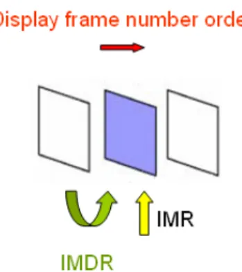
Figure 5: Case 1 is detected by using IMDR and IMR feature.

Case 2: Brightness variation can be observed only when across multiple frames.

In this case, the two adjacent frames may not produce obvious brightness variations and the frame distances of obvious brightness change exceed to one. So, if the inequality (3) is not satisfied, we set the preceding frame as a temp_frame and check for inequality (5) which is showed as follow.

, where m is called Thr_continuous_frame which denotes the upper bound for the number of the frames that an obvious brightness change must be detected across them; otherwise these frames are not in a gradual transition. If inequality (5) is satisfied for any i in between 1 and m, it means that an obvious brightness change is detected across i succeeding frames, and therefore, all these frames are in fade-out transition. Otherwise, there is no brightness change which is across succeeding frames and we assume there is no fade-out transition occurred, therefore, finds out the next one fade-out start point.

The figure 6 shows follow the situation of Case 1 and the detail descriptions are shown in the flowchart of figure 7.

)

5

(

1

_

,

temp

i

Thr

IMDR

for

i

m

temp

.

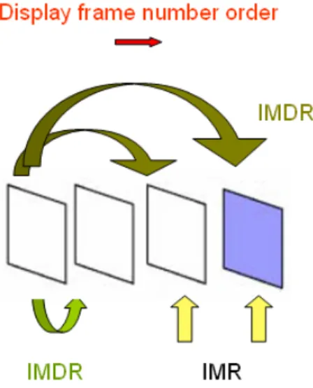
Figure 6: Case 2 is detected by using IMDR and IMR feature.

The flowcharts for Case 1 and Case 2 detection algorithm are shown in figure 7(a) and 8(b) respectively. The Case 2 preprocessing in Case 1, we set the preceding frame as a temp_frame in order to calculate the IMDR between the next frame F(t+1) and the previous frame F(t-1) and uses the threshold Thr_continous_frame to avoid false alarms.

Figure 7(b): The flowchart of Case 2 detection algorithm.

In figure 8(a), x-axis and y-axis which are denoted IMDR and accumulative ratio respectively and in order to observe IMDR change which is caused by brightness change, we use IMDR of adjacent frames in fade-out transitions for test sequence “casino_royale” to observe the distribution of IMDR during fade out transition. When Thr_IMDR = -26, there are 90% probabilities that the frame has an obvious brightness change.

In figure 8(b), x-axis and y-axis which are denoted IMR and accumulative ratio respectively. Similarly, when Thr_IMR = 24, there are almost 90% probabilities that the frame has an obvious brightness change.

(a)

(b)

Figure 8: (a), (b) The experimental results of IMDR ratio and IMR ration during fade out shot transitions.

(III) Edge Direction Similarity Detection

During a fade out shot transition period, the brightness variations are generated between the frames. However, when a frame is affected by brightness variations, the brightness variations are not uniform for each pixel on the affected frame because the film shooting skills and the difference of backgrounds. We used the local area features by dividing the frame image into 16 sub-images (or say windows), and dividing every macroblock into 16 4x4 sub_blocks

Generally, the edge information of the two frames which are affected by brightness variations is very similar. The intra prediction feature of H.264/AVC provides information for the edge direction information. Thus, we explored the intra prediction edge similarity (FADES_IPES) between two frames effected by brightness variations to detect fade out shot transition.

The conception of the FADES_IPES algorithm:

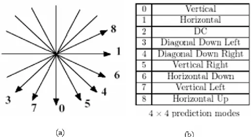
When a macroblock is INTRA 16x16 prediction mode, we assign the edge direction value of INTRA 16x16 prediction mode to each 4x4 sub_block. Otherwise, this macroblock is INTRA 4x4 prediction mode, the 16 4x4 sub_blocks have the same edge direction value of INTRA 4x4. The edge direction angle of each 4x4 sub_block is defined by arctan and showed in figure 9. There are nine modes for INTRA 4x4 prediction mode, so nine different edge direction angles are possible.

Figure 9: (a) The nine different edge direction slopes for INTRA 4x4 prediction modes. (b) The nine different INTRA 4x4 prediction modes.

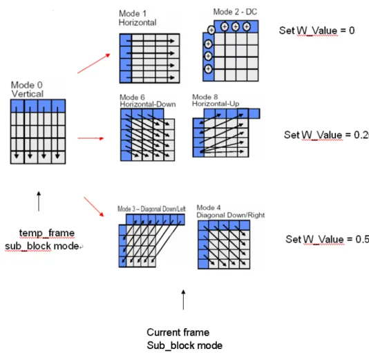
After the brightness change detection, we will detect the two frames which have obvious brightness variations. We compared the edge direction values of co-located 4x4 sub_blocks between the two frames by using the edge slope similarity. Firstly, if the co-located 4x4 sub_blocks of detected two frame are all INTRA prediction mode, it represents a matched pair.. For matched 4x4 sub_blocks, setting the weight value (W_Value) to {0, 0.25, 0.5, 0.75, 1} according the following rules. The bigger W_Value denotes the more edge slope similarity between the two matched 4x4 sub_blocks.

Rules for W_Value setting:

Rule 1: If anyone of a matched pair is INTRA 4x4 DC mode.

The INTRA 4x4 DC mode represents a non_edge prediction. Thus, if only one sub_block mode is INTRA 4x4 DC mode, we set W_Value to zero. Otherwise, the two sub_blocks of a matched pair are all INTRA 4x4 DC mode and we set W_Value to 1.

Set W_Value = 1 : The edge direction slope angle difference of a matched pair is 0. Set W_Value = 0.75: The absolute value of edge direction slope difference of a matched pair is 22.5.

Set W_Value = 0.5: The absolute value of edge direction slope difference of a matched pair is 45.

Set W_Value = 0.25: The absolute value of edge direction slope difference of a matched pair is 67.5.

Set W_Value = 0: The absolute value of edge direction slope difference of a matched pair is 90.

For example to set W_Value in figures 10 and 11:

Figure 11: The examples for W_Value setting

The steps of the FADES_IPES algorithm:

Step1: Set weight value (W_Value) for each matched sub_block pair

Firstly, we set W_Value by comparing the matched 4x4 sub_blocks of the two frames (temp_frame and current frame) which are detected in by brightness change detection step.

Step2: Calculate the average of the sum of W_Value (ASWV) for each windows After step1. the W_Values of matched 4x4 sub_blocks are all set. In order to take the feature of the local area into considerations, we calculate the average of the sum of W_Valure (ASWV) for 16 windows of the frame. The ASWV for the i-th window, say ASWVi, isdefined as following equation (6), and (8):

, where Ni_matched represents the number of matched 4x4 sub_blocks in ith window.

The calculated ASWV values represent the edge similarity between windows. The bigger ASWV value denotes higher edge similarity between windows.

Step3: Judge the edge similarity of frames

In this step, the two thresholds Thr_ASWV and Thr_window are used to decide whether the edge similarity of the two frames is high or not. For the 16 windows in the frame, we count the number of windows (windows_count) that meet condition (9). Then, if the windows_count is hold for the condition (10), it denotes the edge similarity of the two frames is high and passes the FADES_IPES algorithm. Otherwise, the edge similarity of the two frames is low and we judge that the current frame does not belong to a fade out shot transition. In order to choice appropriate Thr_ASWV and Thr_window thresholds, we collect ASWV and windows_count information from 28 fade out shot transitions in stream “casino_royale”. The statistical results are shown in figure 12 and 13, where almost ASWV ratios are higher than 46%, so we set Thr_ASWV to 46. Similarly, in figure 13 the experimental results shows that the windows_count of fade out shot frame are almost exceed to 6, so the Thr_window is set to 6.

)

8

(

_matched

N

i

SWV

i

i

ASWV

=

)

6

(

_

1

_

∑

=

=

matched

i

N

j

j

Value

W

i

SWV

casino_royale 0 10 20 30 40 50 60 70 80 90 100 0 1 2 3 4 5 6 7 8 9 10 11 12 13 14 15 16 windows_count A cc um ula ti ve R at io ( % ) casino_royale

Figure 12: The experimental results of the ASWV

Figure 13: The experimental results of the ASWV

)

10

(

_

_

)

9

(

_

window

Thr

count

Windows

ASWV

Thr

ASWV

≥

≥

(IV) End Point Detection

At the end of fade out period, the frame images became solid color images generally. There are two cases should be discussed as follows:

Case 1: Slow fade out shot transition

In this situation, frame images became solid color images slowly during the fade out period and the solid color images remain for more than one frames. In this case, it will produce a lot of P_SKIP mode macroblocks near the fade out end point. Thus, we used the P_SKIP MB Ratio (PMR) which is defined in equation (11) to detect the fade out end point.

If a frame has passed the FADES_IPES algorithm, it represented that the edge similarity of this frame and some frame in the fade out transition is very high. This frame should belong to a fade out shot transition. Then, we compare the PMR value of this frame with a predefined threshold Thr_PMR. If the PMR value of this frame is equal or higher than Thr_PMR, the current frame is the fade out end point. In our experimental result, there are 90% probability that the PMR ratio will exceed to 95% at the end point of a fade out shot transition. Thus, we set Thr_PMR to 90%.

)

11

(

_

number

MBs

total

number

MBs

SKIP

P

PMR

=

Case 2: Fast fade out shot transition

In this situation, frame images became to solid color images fast during the fade out period and the solid color images are even not obvious. That is, the fade out shot transition does not finish completely, and the fade out end point is not a solid color image. So, we cannot use the PMR feature to detect the fade out end point because of the P_SKIP mode MBs do not increase dramatically.

When a fade out end point occurred, the edge similarity is very low between the end point of the fade out shot transition and the first frame of the new shot. So, we used this feature. Firstly, we used a frame_num_array (array size is set to 4) to record the frame numbers which are candidate fade out frame numbers detected by FADES_IPES algorithm and updated it when any frame passed the FADES_IPES algorithm. Secondly, when a fade out start point is fought, execute the edge direction similarity detection frame by frame. Then, once the FADES_IPES algorithm failed for two adjacent frames, we check the contents of frame_num_array. If the frame number distance of all the two adjacent contents of the frame_num_array is smaller than 5, the fade out end point is detected. That is,

If current_frame>frame_num - frame_num_array[3] 4 and frame_num_array[3] - frame_num_array[2] 4 and

frame_num_array[2] - frame_num_array[1] 4 and frame_num_array[1] - frame_num_array[0] 4 and

start_point_frame_num frame_num_array[0] Then, a fade out end point is detected.

≤ ≤ ≤ ≤ ≤

3.2 The flowchart overview of fade out shot transition

detection algorithm:

The figure 14 is shown that the complete detail flowchart of the fade out shot transition detection algorithm..

3.3 Fade In Shot Transition Detection Algorithm

Similarly, the proposed fade in detection algorithm also has four steps start point detection, brightness change analysis, edge direction similarity check, and end point detection respectively. The functions of brightness change analysis and edge direction similarity check steps are the same with fade out shot detection algorithm. Thus, in this section, we only introduce start point detection and end pint detection steps.

Start Point Detection:

During the fade in shot transition, a shot gradually appears and end with a clear color image. In a general fade in transition, there are also brightness variations between the first frame and the second frame. So, the conception is the same as start point of fade out shot detection algorithm, we use the feature of IMDR to detect the start point in a fade in shot transition. In order to decide an appropriate IMDR threshold for fade in start point, we collect information from three sequences: “casino_royale”, “jihnrambo”, and “king_kong”. Similarity, for each sequence, we calculate the IMDR value for each fade in start point frame and conduct the start point ratio for each IMDR value. The statistical results are shown in figure 15 where it displays the accumulative start point ratio as a function of IMDR values, ranging from 0 to 100. When a fade in start point occurred, there are 75% probabilities that Thr_IMDR values, ranging from 26 to 98, Thus, we set 26 <= Thr_IMDR <= 98 for fade in start point detection.

Figure 15: The experimental results of the start point of IMDR value for video sequences “johnrambo”, “rescue_dawn”, and “casino_royale” respectively.

End Point Detection:

At the end of fade out period, frame images became to more and more clear successively. Because frames are more and more clear, the numbers of INTRA macroblocks are more and more decrease. It causes that the IMDR value dramatic decreases and be a negative value. Thus, we use IMDRi-1,i, IMDRi-2,i-1, and IMDRi-3,i-2

to detect the end point in fade out shot transition. The figure 16 shows the IMDRi-1,i,

IMDRi-2,i-1, and IMDRi-3,i-2.

Figure 16: The IMDRi-1,i, IMDRi-2,i, and IMDRi-3,i.

0 10 20 30 40 50 60 70 80 90 100 0 20 40 60 80 100 IMDR Ratio (%) A cu um ula tiv e R atio ( % ) casino_royale johnrambo king_kong

Firstly, we also use a frame_number_array (array size is set to 4) to record the frame numbers which are candidate frames of fade-in shot transition detected by FADE_IPES algorithm and updated when any frame passed the FADE_IPES algorithm. Secondly, when a fade in start point fought, to execute the edge direction similarity check frame by frame. Once the FADE_IPES algorithm failed for the two adjacent frames, we check the content of frame_num_array that has mentioned in the section of fade out end point detection. If check is meet and anyone of the following three inequalities (12), (13), and (14) is hold, the i-th frame is the end point of a fade in shot transition.

, where the Thr_IMDR1, Thr_IMDR2, and Thr_IMDR3 are predefined thresholds. In order to decide these three appropriate thresholds for end point detection, we collect information from the sequence “casino_royale”. For the sequence, we calculate the IMDRi-1,i, IMDRi-2,i-1, and IMDRi-3,i-2 values for each end point and

conduct the end-point ratio for each IMDR value. In figure 17, the experimental results show that there are 88%, 79%, and 65% probabilities that when IMDRi-1,i,

IMDRi-2,i-1, and IMDRi-3,i-2 values are smaller than -18, -9, and 4 respectively. Thus,

we set thresholds Thr_IMDR3 = 4, Thr_IMDR2 = -9, and Thr_IMDR = -18.

)

14

(

3

_

2

,

3

)

13

(

2

_

1

,

2

)

12

(

1

_

,

1

IMDR

Thr

i

i

IMDR

IMDR

Thr

i

i

IMDR

IMDR

Thr

i

i

IMDR

≤

−

−

≤

−

−

≤

−

Figure 17: The experimental results of IMDRi-1,i, IMDRi-2,i-1, and IMDRi-3,i-2 values.

3.3 Cut Shot Change Detection Algorithm

This section presents the proposed cut shot change detection algorithm, we combined the enhanced PHD methods with revised IPES algorithm (which is called CUT_IPES algorithm) There are two steps to detect the cut shot change:

Step 1: The enhanced PHD methods

The original PHD methods are mentioned in chapter 2. The conception of the original PHD methods utilized the features that the P_mode and B_mode macroblocks increase between the first and the second frame of the new shot. However, our enhanced cut shot change detection algorithm explores the features that the P_mode and B_mode macroblocks decrease between the first frame of the next new shot and the last frame of the current shot. Thus, we change the PHD threshold (Thr_PHD)

according to statistical information in figure 18. In figure 18, we counted the PHD values for three different test video sequences. When a cut change occurred, the PHD value is almost smaller than -0.39. We set the Thr_PHD to -0.39 and determined a frame, F(t), as a cut change candidate using following condition (15).

Figure 18: The experimental results of the PHD threshold.

Step 2: The edge direction similarity algorithm

In this step, we modify the proposed FADE_IPES algorithm mentioned in fade out shot transition algorithm to detect the cut shot change. When a new cut shot change occurred, there are many differences with the content texture. Thus, after a cut candidate decided by step 1, the edge direction similarity algorithm is executed to detect the cut candidate with the previous one frame. We count the number of

)

15

(

_

)

)

1

(

,

)

(

(

F

t

F

t

Thr

PHD

PHD

−

≤

that the edge of almost co-located areas are not the same, and the cut candidate, F(t), is decided as a cut shot frame. We change the Thr_ASWV and Thr_windows for cut shot change detection. Similarly, we collect ASWV and Windows_count information from the cut shot change in stream “casino_royale” in order to choice appropriate Thr_ASWV and Thr_window thresholds. The figures 19 and 20 show the statistical results of the thresholds Thr_ASWV and Thr_windows respectively. The figure 19 shows that the almost ASWV value are smaller than 50%, so we set Thr_ASWV to 50. Similarly, in figure 20, the experimental results shows that the windows_count of fade out shot frame are almost exceed to 9, so the Thr_window is set to 9.

Figure 19: The experimental results of the ASWV

)

17

(

_

_

)

16

(

_

window

Thr

count

Windows

ASWV

Thr

ASWV

≥

≤

Figure 20: The experimental results of the windows_count

Chapter 4 Experimental Results

4.1 Performance Evaluation Criteria

The section presents the experimental results of the proposed algorithm. The performance evaluation of shot change detection algorithms measured by comparing the output of the algorithm with the ground truth which is obtained manually by human eye’s inspection. The comparison is based on Recall NR and Precision NP

given by the following equations

, where Nc represents the number of correct shot detection Nc, Nm denotes the number

of missed shot detection, and Nf represents the number of false shot detection

Recall NR denotes the percentages of the number of the existing shots that are

detected, and Precision NP means that how many percentages of the detected shots are

correct.

However, for gradual shot transitions, the detection algorithm cannot be evaluated by using Recall and Precision because they can not describe how precisely a gradual shot transition is detected. For this reason, we have defined the Gradual Shot Transition Recall GR and the Gradual Shot Transition Precision GP, both are

defined in the following equations:

%

100

*

f

N

c

N

c

N

p

N

+

=

%

100

*

m

N

c

N

c

N

R

N

+

=

,

where NCGi stands for the number of correctly detected frames in the gradual shot Gi,

NmGidenotes the number of missing frames in the gradual shot Gi , and NfGirepresents

the number of false detected frame in the gradual shot Gi .

4.2 Test Video Sequence and Evaluation

Enviroments

We compared our fades shot detection algorithm and cut shot detection algorithm with K.Schoffmann et al. [11] algorithm, Bohyun Hong et al. [12] algorithm, and J. Sastre et al. [14] algorithm respectively. All the algorithms are implemented by modifying H.264/AVC JM 13.1. GOP structure is set IPPP, frame rate is set 30 frames/sec, frame resolution is set 4CIF (704x576), QP is set 28, and Multiple Reference Frame number is set to five. The video sequences used in our experiments include five movie-trailers “rescure_dawn”, “casino_royale”, “johnrambo”, “kingkong”, and “300P” which are easily downloaded from some movie trailers websites and one test video sequence “A” which is captured from the movie “sexual emergency” for 136 second. The number of shots and the shot types in these

∑

=

+

=

N

c

i

Gi

N

_m

Gi

c

N

Gi

c

N

of

average

R

G

1

∑

=

+

=

N

c

i

Gi

f

N

Gi

c

N

Gi

c

N

of

average

P

G

1

sections are summarized in Table 4. In order to show the effectiveness and robustness of the proposed fades shot transition algorithm, the test video sequences are encoded various bit-rates by adjusting the QPs which are set to 28, 30, and 32 respectively to detect fades shot transition.

Table 3: The number of shots and the shot types

4.3 Performance Comparison with

Different Fades Detection Methods

We compared our fades shot transition algorithm with K.Schoffmann et al. [11] algorithm. The experimental results for each test sequence are shown in Table 5. From the experimental results, it is observed that although K. Schoffmann et al. algorithm can detect the boundaries of fades shot transitions, the Recalls and Precisions are not good effectiveness enough and the Recalls are even worse.

On the other hand, our proposed fades shot transitions algorithm can detect those fades shot transitions well and is able to identify the shot types, the fade in/out from fades shot transitions. The average Recall and Precision of our proposed algorithm are 88.96% and 84.382% respectively. The average Gradual Recall GR and Gradual

Precision GP are respective 90.892% and 83.49%. The missing fades shots are caused

by very slow fades shot transitions and some incomplete fades shot transitions which denoted that the last frame of a fade-out shot is not a solid image or the last frame of fade-in shot is an unclear image. The false alarm of fades shots are caused by cut shots of the very high motion and some kind of dissolves shot transitions.

Table 5 (a): The experimental results of proposed fade out/in detection algorithms.

Table 5(b): The experimental results of K. Schofmann et al. proposed different fade shot transitions algorithms.

P

G

R

G

R

G

G

_P

4.4

Performance Comparison with

Different Shot Change Detection

Methods

In this subsection, we compared our proposed cut shot detection algorithm and fades shot transitions algorithm with the methods proposed by Bohyun Hong et al. [12], J. Sastre et al. [14], and K. Schofmann et al. [11]. From Table 6, the average Recall and Precision of our proposed algorithms are almost higher than the other algorithms. Although the average Recall of the proposed algorithm by Sastre is a little larger than our proposed algorithm, its average Precision is very low. Because of Sastre proposed algorithm doesn’t have meticulous method to eliminate false alarms generated by the adaptive threshold detection. This situation caused Recall and Precision that can’t attain a good trade-off. The average Recall and Precision of our algorithm are 87.68% and 90.58% respectively, this results show our proposed algorithms can detect shot change very well. Moreover, the proposed algorithm can identify mark the type of a shot and the boundaries of a shot clearly, but the other algorithms can’t.

(a)

(b)

Table 6: (a), (b), (c), and (d) are the experimental results of shot change algorithms proposed by Bohyun, Sastre, Klaus, and us respectively.

4.5 Performance Comparison between

Different Shot Detection Methods and

our enhanced Shot change Detection

Methods

We combine the proposed fade out/in shot detection algorithm and CUT_IPES algorithm with the Bohyun Hong et al. [12] methods, and J. Sastre et al. [14] methods respectively. We execute the proposed fade out/in shot detection algorithm to find the fade shot transition frames, then, performs the Bohyun Hong et al. [12] methods, and J. Sastre et al. [14] methods with proposed CUT_IPES algorithm for the remaining frames. Table 7 shows that by incorporating Sastre’s and Bohyun’s methods with the proposed CUT_IPES algorithm, the average Recall and Precision improve dramatically, with the increase of the Precision up to 19%. Because the proposed CUT_IPES algorithm which judges the edge similarity very precise and works on shot change detection algorithm efficaciously. So, the proposed CUT_IPES

produce ambiguous results.

(a): The experimental results of Sastre’s methods with and without proposed CUT_IPES algorithm

CUT_IPES algorithm

(c)

charts of Recall and Precision by comparing with different shot change detection algorithm.

4.6 Performance Evaluation for the

Video Sequences with Different

Bit-Rates

In order to manifest the effectiveness and robustness of the proposed fades shot detection algorithms, each of the test video sequences is encoded into three different various bit-rates by adjusting the values of quantization parameter in the encoder of H.264/AVC. The experimental results of the proposed fade out/in detection algorithms in various bit-rates for two different video sequences which are shown in Table 8. It demonstrates that performs good effects under various bit-rates conditions.

(b)

Table 8: (a), (b) The experimental results of different video test sequences under various different bit-rates.

Chapter 5. Conclusion and Future Works

In this thesis, we have proposed an efficient and robust shot change detection method for H.264/AVC video bitstreams. The method includes two different types shot change detection algorithms: the fades shot detection algorithm and the cut shot detection algorithm respectively. Fades shot detection algorithm explored some features likes the INTRA MBs difference ratio, INTRA MBs ratio and edge direction similarity to detect fade in/out shot transitions. Cut shot detection algorithm used PHD (partition histogram difference) and edge direction similarity to precisely detect cuts change.

By the comparison with other shot change detection methods on several video sequences, the experimental results showed the effectiveness of our proposed shot

proposed shot change detection method still worked effectively and robustly.

Future works are shown as follows:

1. Improve the false alarms false caused by the very high motion cut shots and some kind of dissolves shot transitions.

2. Research the other types of shots such as dissolves shot transition.

Bibliography

[1] H. J. Zhang, J. Wu, D. Zhong, and S. Smoliar, “An integrated system for content-based video retrieval and browsing,” Pattern Recognit., vol.30, pp. 643–658, 1997.

[2] Huang, C.L., and Liao, B.Y.: A Robust Scene-Change Detection Method for Video Segmentation, IEEE Transactions on Circuits and System for Video Technology, vol. 11, no. 12, (2001) 1281-1288

[3] P.N. Hashimah, L. Gao, R. Qahwaji, J. Jiang: An Improved Algorithm for Shot Cut Detection. In: Proc. of VCIP: Visual Communications and Image Processing, Vol. 5960, Bellingham, WA (2005) 1534-1541

[4] B.T. Truong, Ch. Dorai, S. Venkatesh: New Enhancements to Cut, Fade, and Dissolve Detection Processes in Video Segmentation. In: Proc. of the 8th ACM international conference on Multimedia, Marina del Rey, California, United States (2000) 219 - 227

[5] S. Porter, M. Mirmehdi, B. Thomas: Detection and Classification of Shot Transitions. In: British Machine Vision Conference (BMVC) (2001) 73-82

[6] S. C. Pei and Y. Z. Chou, “Efficient MPEG compressed video analysis using macroblock type information,” IEEE Trans. Multimedia, vol. 1, no. 4, pp. 321–333, Dec. 1999.

[7] A. Akutsu, “Video indexing using motion vectors,” in Proc. SPIE Vis. Commun. Image Process., 1992, vol. SPIE 1818, pp. 1522–1530.

[8] B. L. Yeo and B. Liu, “Rapid scene analysis on compressed video,” IEEE Trans. Circuits Syst. Video Technol., vol. 5, no. 6, pp. 533–544, Dec. 1995.

[10] Bita Damghanian1, Mahmoud Reza Hashemi2, and Mohammad Kazem Akbari1: A Novel Fade Detection Algorithm on H.264/AVC Compressed Domain, LNCS 4903, Springer-Verlag Berlin Heidelberg 2008 pp. 1159 – 1167

[11] Klaus Sch¨offmann and Laszlo B¨osz¨ormenyi: Fast Segmentation of H.264/AVC Bitstreams for On-Demand Video Summarization, LNCS 4903, Springer-Verlag Berlin Heidelberg 2008 pp. 265–276

[12] Bohyun Hong, Minyoung Eom, Yoonsik Choe: Scene Change Detection using Edge Direction based on Intra Prediction Mode in H.264/AVC Compression Domain,in Proc.IEEE INT. Region 10 Conference 2006

[13] B. S. Manjunath, Philippe Salembier, Thomas Sikora, "Introduction to MPEG-7 Multimedia Content Description Interface", Wiley

[14] J. Sastre, P. Usach, A. Moya, V. Naranjo, and J. Lopez. Shot Detection Method For Low Bit-Rate H.264 Video Coding. In Proceedings of the 14th European Signal Processing Conference, Eusipco 2006, Florence, Italy, September 2006

[15] S. C. Pei and Y. Z. Chou, “Efficient MPEG compressed video analysis using macroblock type information,” IEEE Trans. Multimedia, vol. 1, no. 4, pp. 321–333, Dec. 1999.

[16] P. Bouthemy,M. Gelgon, and F. Ganansia, “A unified approach to shot change detection and camera motion characterization,” IEEE Trans. Circuits Syst. Video Technol., vol. 9, no. 7, pp. 1030–1044, Oct. 1999.

[17] K. Shen and E. J. Delp, “A fast algorithm for video parsing using MPEG compressed sequences,” in IEEE Int. Conf. Image Process., Oct.1995, pp. 252–255.