利用虛擬實境駕駛模擬進行雙重任務下分心之腦波反應研究

(1)

國立交通大學

電機與控制工程學系

碩士論文

利用虛擬實境駕駛模擬進行雙重任務下分心之

腦波反應研究

EEG Dynamics in Response to Distraction in

Virtual Reality Driving Simulation

研究生：林弘章

指導教授：林進燈博士

陳右穎博士

(2)

利用虛擬實境駕駛模擬進行雙重任務下分心效應之

腦波反應研究

EEG Dynamics in Response to Distraction in Virtual Reality

Driving Simulation

研究生：林弘章 Student：Hong-Zhang Li

n

指導教授：林進燈博士

Advisor：Dr. Chin-Teng Lin

陳右穎博士

Dr. Yu-Ying Chen

國立交通大學

電機與控制工程學系

碩士論文

A Thesis

Submitted to Department of Electrical and Control Engineering

College of Electrical and Computer Engineering

National Chiao Tung University

in Partial Fulfillment of the Requirements

for the Degree of Master

in

Electrical and Control Engineering

June 2007

Hsinchu, Taiwan, Republic of China

(3)

利用虛擬實境駕駛模擬進行雙重任務下分心之

腦波反應研究

學生：林弘章

指導教授：林進燈博士

陳右穎博士

國立交通大學電機與控制工程研究所

中文摘要

駕駛者分心已經證實是造成車禍發生的重大原因之一。因此，本論文以腦電波(Electroencephalogram, EEG)來探討駕車行為下人類分心效應的腦部反應變化。研究中使用虛擬實境技術之動態駕車裝置，來模擬真實之駕車環境。在此實驗中，我們設計非預期性的車子偏移與數學問題的出現，來探討雙重任務所造成的分心效應。同時，為了進一步探討偏移和數學此二種任務在不同時間出現下的相互影響程度，我們設計了五個在事件出現時間點上有差異的狀況，並找出二種任務在不同的出現時間點，所造成腦電波上分心效應的反應變化。EEG 訊號經過獨立成份分析(Independent Component Analysis, ICA)後分離成數個獨立的訊號源，再利用事件相關頻譜擾動(Event Related Spectral Perturbation, ERSP) 來計算事件發生前與後的頻譜變化，並經由此來觀察腦不活動在不同時間點上的頻譜差異。結果發現在額葉的區域，Theta 頻帶 (5~7.8 Hz) 和 Beta 頻帶 (12.2~17 Hz) 的能量會因為分心效應而增強。在枕葉區域，觀察到因為視覺刺激所誘發的反應現象以及因為回答數學問題按按鍵所產生的放鬆現象。在運動皮質區觀察到在 Alpha 頻帶因為事件誘發的能量抑制。以上所發現的腦部活化結

(4)

果在不同受測者均可以觀察到相同的反應。由以上這些結果我們能證明在駕駛事件與數學題目出現時間點有差異的狀況下，行為反應和腦波反應也相對應有變化。此一實驗結果也發現在額葉區域的 Theta 頻帶能量增強變化可以作為日後偵測駕駛者在實際駕駛中是否有分心的指標。關鍵字：分心、雙重任務、腦電波、額葉、Theta 頻帶、數學、事件相關頻譜擾 動、獨立成份分析

(5)

EEG Dynamics in Response to Distraction in

Virtual Reality Driving Simulation

Student:

Hong-Zhang Lin

Advisor: Dr. Chin-Teng Lin

Dr. Yu-Ying Chen

Department of Electrical and Control Engineering

National Chiao Tung University

Abstract

Driver distraction has been recognized as a significant cause of traffic incidents. Therefore, the aim of this study was to investigate Electroencephalography (EEG) dynamics in response to distraction during driving. To study human cognition under specific driving task, we used Virtual Reality (VR) based driving simulation to simulate events including unexpected car deviations and mathematics questions (math) in real driving. For further assessing effects of the stimulus onset asynchrony (SOA) between the deviation and math presented on the EEG dynamics, we designed five cases with different SOA. The scalp-recorded EEG channel signals were first separated into independent brain sources by Independent Component Analysis (ICA). Then, the Event-Related-Spectral-Perturbations (ERSP) measuring changes of EEG power spectra was used to evaluate the brain dynamics in time-frequency domains. Results showed that increases of theta band (5~7.8 Hz) and beta band (12.2~17 Hz) power were observed in the frontal cortex. For occipital components, we found the pattern of visual induced brain activities and rebounds from the button press. In motor components, we found alpha suppressions time-locked to event onsets. All the above results were consistently observed across 11 subjects. Results demonstrated that

(6)

reaction time and multiple cortical EEG sources responded to the driving deviations and math occurrences differentially in the stimulus onset asynchrony. Results also suggested that the phasic theta increase in frontal area could be used as the distracted indexes for early detecting driver’s inattention in the real driving in the future.

Keyword: Distraction, Dual task, Frontal lobe, Theta band, Mathematics, Mental

(7)

誌謝

本論文的完成，首先要感謝指導教授林進燈博士以及共同指導教授陳右穎博士這兩年來的悉心指導，讓我學習到許多寶貴的知識，在學業及研究方法上也受 益良多。另外也要感謝口試委員們的建議與指教，使得本論文更為完整。 特別感謝美國加州聖地牙哥大學的鐘子平教授、段正仁教授及黃瑞松學 長，給予我研究上最大的協助，從實驗設計、實驗分析、實驗結果討論到論文撰 寫，給我最專業的意見跟看法。 另外，我要感謝腦科學研究實驗室的全體成員，沒有他們也就沒有我個人的 成就。特別感謝曲在雯博士、梁勝富教授、蕭富仁、林文杰教授給予我在各方 面的指導，無論是研究上疑難的解答、研究方法、寫作方式、經驗分享等惠我良多。另外要感謝明達、仲良、俊傑、智文、德瑋、林玫同學，在過去兩年研究生活中同甘共苦，相互扶持。此外，我也要感謝陳玉潔學姊、林君玲學姐、柯立偉學長、趙志峰學長、陳世安學長與黃騰毅學長在研究上的幫助，還有感謝德正、尚文、青甫、柏銓、玠瑤、孟修、依伶，在過去這一年中的相伴。同樣地也感謝 實驗室助理 Amy 、Apple、May 在許多事務上的幫忙。 謹以本文獻給我親愛的家人與親友們，以及關心我的師長，願你們共享這份 榮耀與喜悅。

(8)

List of Tables

Table-1: The Specification of driving simulator ...8

Table-2: Specifications of NuAmps...11

Table-3: The normalized response time to deviation and math ...32

(11)

List of Figures

Fig. 2-1: The illustration of the experimental setup including the dynamic VR driving

environment and the EEG-based physiological measurement system. ...5

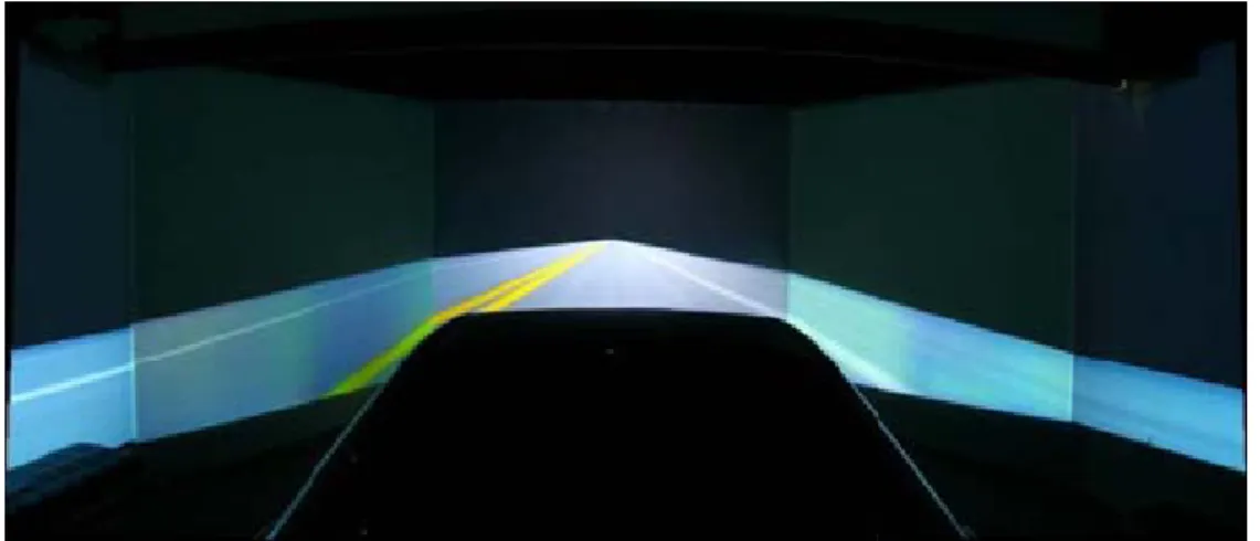
Fig. 2-2: Pictures showed the dynamic VR driving environment, in the Brain Research Center of National Chiao Tung University, Taiwan, and ROC...7

Fig. 2-3: The picture showed the configuration of the 3D surrounded scene...8

Fig. 2-4: The picture showed the overview of surrounded VR scene...9

Fig. 2-5: Schematic pictures showed the lateral (A) and top view (B) of international 10-20 system of electrode placement [24]. ...9

Fig. 2-6: The picture showed the setup of the physiological recording containing the NuAmps EEG amplifier and the electrode cap...10

Fig. 2-7: The picture showed the Fastrak 3D Digitizer...11

Fig. 2-8: The photomicrograph showed the simulated high way scene...12

Fig. 2-9: The illustration of the high way scene.. ...13

Fig. 2-10: The illustration of the experimental paradigm.. ...14

Fig. 2-11: The illustration of the deviation event...14

Fig. 2-12: The illustration of the relationship between the deviation onset and math occurred...15

Fig. 3-1: The flowchart of analyzing the behavioral data...18

Fig. 3-2: The flowchart showed the EEG signal processes...19

Fig. 3-3: The illustration of the ERP analysis.. ...20

Fig. 3-4: Illustration of the concept of ICA process...21

Fig. 3-5: The picture showed the typical example of scalp topography of ICA decomposition...22

Fig. 3-6: The illustration of procedures in ERSP analysis. ...25

Fig. 3-7: The flowchart of component clustering by using K-means algorithm...27

Figure 3-8: The typical example of the component clustering result. ...27

Fig. 4-1: Bar charts of the averaged response time to the deviation (A) or the math (B) onsets between four cases. ...29

Fig. 4-2: Bar charts of normalized response time to the deviation (A) and math (B) presented between 5 cases across 11 subjects...31

Fig. 4-3: Scalp map topographies of ICA decomposition of subject-4...33

Fig. 4-4: The illustration of the component maps and their corresponded dipole locations ...34

Fig. 4-5: Illustration of the typical example of six ICs and their power spectra from five different cases ...36

(12)

Fig. 4-6: Single subject data. The comparison of total power spectra between single- and dual-task in the central midline component. ...37 Fig. 4-7: Single subject data. The comparison of power spectral baselines between

single- and dual-task cases in the motor component. ...38 Fig. 4-8: Single subject data. The comparison of power spectra between single- and

dual-task cases in the parietal component...38 Fig. 4-9: Single subject data. The comparison of power spectra between single- and

dual-task cases in the frontal component...39 Fig. 4-10: Single subject data. The ERSP plots of the single-task cases in the frontal

component...41 Fig. 4-11: Single subject data. The ERSP plots of the dual-task cases in the frontal

component...42 Fig. 4-12: Single subject data. The ERSP plots of the five cases in the frontal

component...43 Fig. 4-13: Single subject data. The ERSP plots of the single-task cases in the motor

component...44 Fig. 4-14: Single subject data. The ERSP plots of the five cases in the motor

component (p<0.05)...45 Fig. 4-15: Single subject data. The ERSP plots of the five cases in the parietal

component (p<0.05)...46 Fig. 4-16: Single subject data. The ERSP plots of the five cases in the occipital

component (p<0.05)...48 Fig. 4-17: The scalp maps...49 Fig. 4-18: The grand mean of total power spectra for epochs from five cases in the

frontal cluster across 10 subjects. ...51 Fig. 4-19: The comparison of the averaged power around the 5~7.8 Hz and 12.2~17

Hz between the single task and dual tasks across 10 subjects in the frontal

component...52 Fig. 4-20: The grand mean of the total power spectra for epochs from five different

cases in the right motor cluster across 6 subjects. ...53 Fig. 4-21: The comparison of the averaged alpha power between the single tasks and

dual tasks in the motor cluster...54 Fig. 4-22: The ERSP images of frontal cluster for five cases...55 Fig. 4-23: The comparison of total power in cross-subject averaged ERSP images in

frontal component between cases. ...56 Fig. 4-24: Effects of distraction on onsets of theta and beta increases. ...57 Fig. 4-25: The grand mean of cross-subject averaged ERSP images ...57 Fig. 4-26: The comparison of total power in cross-subject averaged ERSP images ...58

(13)

Fig. 4-27: The distracted effects on latencies of alpha suppression measured averaged ERSP images of the motor components...59 Fig. 4-28: The grand mean of averaged ERSP images ...59 Fig. 4-29: The averaged ERPs of the left (left block: 7 subjects) and right (right block: 5 subjects) occipital clusters for five cases. ...60 Figure 5-1: Picture showed the principle fissures and lobes cerebrum ...63

(14)

1 I. Introduction

Distraction and inattention of drivers have been identified as the main leading causes of car accidents. The U.S. National Highway Traffic Safety Administration has identified driver distraction as a high priority area about 30% [1]. Driver distraction by whatever cause is a significant contributor to road traffic accidents [2] [3]. Driving is a complex task in which several skills and abilities are involved simultaneously. Monitoring drivers’ attention related brain resources is still a challenge for researchers and practitioners in the field of cognitive brain research and human–machine interaction.

Reasons of distractions found during driving were quite widespread, including eating, drinking, talking with passengers, use of cell phones, reading, fatigue, problem-solving, and using in-car equipment. Recently, commercial vehicle operators with complex in-car technologies (such as navigation, road traffic information, mobile telephones and in-vehicle entertainment systems) are also at increased risk since drivers may become increasingly distracted in the years to come, thus making it likely that the problem of driver inattention [4] [5]. Some literatures studied the behavioral effect of driver’s distraction in car. Tijerina’s study was based on measurement of the static completion time of an in-vehicle task [6]. Similarly, the distraction effect caused by cellular phones during driving has been a focal point of recent in-car applications [7] [8] [9]. Experimental studies have been conducted to assess the impact of specific types of driver distraction on driving performance. While these studies have generally reported significant driving impairment [10] [11], simulator studies cannot provide information about the impact of these decrements on the occurrence of crashes

(15)

resulting in hospital attendance by the driver. Therefore, in order to provide information before the occurrence of crashes we try to investigate the drivers’ physiological responses.

To the aspect of neural physiological investigation, some literatures focused on the brain activities of “divided attention” referring to attention divided between two or more sources of information, such as visual, auditory, shape, and color stimuli. Madden et al. [12] investigated brain activation when subjects were instructed to divide their attention among the display positions within the visual modality. Regional cerebral blood flow (rCBF) activation was found in occipitotemporal, occipitoparietal, and prefrontal regions. And Positron emission tomography (PET) measurements were taken while subjects discriminated between shape, color, and speed of a visual stimulus under conditions of selective and divided attention. The divided condition activated the anterior cingulated and prefrontal cortex in the right hemisphere [13]. In another study, functional magnetic resonance imaging (fMRI) was used to investigate the brain activity during a dual-task (visual stimulus) experiment. This found activation in the posterior dorsolateral prefrontal cortex and lateral parietal cortex [14]. Similarly, the study used electroencephalogram (EEG) to investigate mental arithmetic-induced workload increasing, the finding is power increase in theta band in the region of frontal lobes [15]. And, several neuroimaging studies showed the

importance of the prefrontal network in dual-task management [16] [17]. However,

the above-mentioned studies just investigated the brain activity of dual-task interaction without considering the stimulus onset asynchrony (SOA) problem during driving and the effect of different temporal relationship of stimuli.

The current investigation utilized an array of methodological assessment techniques and compared the sensitivity of each to changes in attention processing requirements as a function of driving task demand. Some literatures of investigated

(16)

the traffic record the electroencephalogram (EEG) to compare the P300 amplitude [18]. During simulated traffic scenarios, resource allocation was assessed through as event-related potential (ERP) novelty oddball paradigm [19]. However, these are just to analyze in time course, we can take one step to analyze the relation between time and frequency course.

The electroencephalogram (EEG) has been used for 80 years in clinical practices as well as basic scientific studies. Nowadays, EEG measurement is widely used as a standard procedure in researches such as sleep studies [20], epileptic abnormalities, and other disorders diagnoses. Comparing to another widely used neuroimaging modality, functional Magnetic Resonance Imaging (fMRI), EEG is much less expensive and has the superior ability of temporal resolution for us to investigate the SOA problems. Furthermore, to avoid the interference and risks of operating an actual vehicle on the road, the use of driving simulation for vehicle design and studies of driver’s behavior and cognitive states is also expanding rapidly [21] [22]. The static driving simulation may be difficult to approach the realistic driving condition, such as the vibrations that would be experienced when driving an actual vehicle on the road. The VR technique allows subjects to interact directly with a virtual environment rather than monotonic auditory and visual stimuli. Integrating realistic VR scenes with visual stimulus is easier to study the brain response to visual attention during driving. Therefore, in recent years, the VR-based simulation combined with electroencephalogram (EEG) monitoring is an innovation in cognitive engineering research [20] [23].

The main goal of this study is to investigate the brain dynamics related to distraction by using EEG and VR-based realistic driving environment. Unlike the previous studies, our experiment has three main characteristics. First, the stimulus onset asynchrony (SOA) experimental design, the different appearance time of dual

(17)

tasks (mathematical questions and unexpected car deviation), has the benefits for us to investigate the driver’s behavioral and physiological response under multiple conditions and multiple distracted levels. Second, the ICA-based advanced signal analysis methods were used to extract the artifact-free brain responses and related cortical location related to the single/dual task. Third, compared with single task, the interaction and effect of dual-task-related brain activities was also investigated. The detailed contents are described in the following sections.

The thesis was organized in 6 chapters. Chapter 1 briefly introduced current knowledge in vestibular system and the goal of the study. Chapter 2 detailed the apparatus and materials of the study. Chapter 2 also described the details of experimental setup, including the time course of event onset asynchrony setup. In chapter 3, we explored the EEG with innovative methods by combining Independent Component Analysis (ICA), time-frequency spectral analysis, power spectrum and component clustering. Chapter 4 showed the results. Chapter 5 discussed and compared our finding with previous studies, and finally we concluded in Chapter 6.

(18)

2 II. Experimental Apparatus

The main purpose of this research was to investigate the EEG features related to distraction in a dual-task experiment. The most concerned issue in dual-task studies was the effect of distraction on driving because it directly related to public safety. For example, using cell-phone, tuning radio or looking at the road-sign could distract the drivers from their driving task and cause serious traffic accidents. However, the driving experiments were very dangerous if they were took place on road. With combining the technology of virtual reality (VR), a driving environment was constructed for the safety of driving experiments in our lab. The VR-based dynamic environment could provide realistic visual and motion stimuli to the subjects. The environment was employed in the setup of dual-task experiment as shown in Fig. 2-1.

Fig. 2-1: The illustration of the experimental setup including the dynamic VR driving environment and the EEG-based physiological measurement system.

(19)

There were three major parts of the architecture: (1) a 3D highway driving scene based on the VR technology, (2) a real vehicle mounted on a 6-DOF motion platform, (3) a physiological signal measurement system with 36-channel EEG/EOG/ECG sensors. The subjects were asked to sit in a real car mounted on the 6-DOF motion platform with their hands holding the steering wheel to control the simulated car in the VR scene. The 30-channel scalp EEG and 4-channel EOG were simultaneously recorded at 1 KHz sampling rate. The details of the experimental setup would be presented in the following sections.

2.1 Dynamic Driving Environment

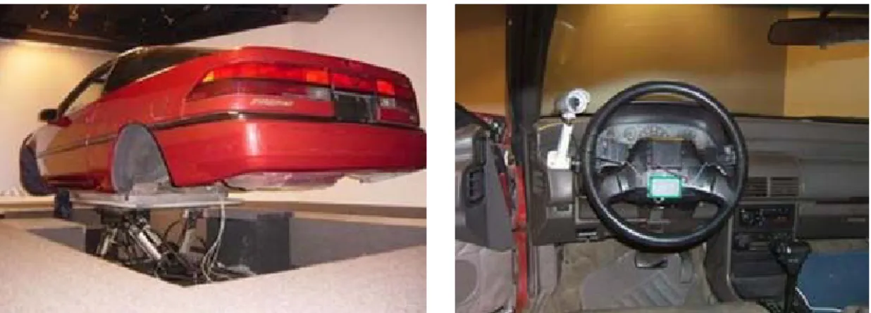
A virtual-reality (VR) based highway-driving environment was used to investigate the changes on drivers’ distraction effect. The VR driving environment includes 3D surround scenes projected by seven projectors and a real car mounted on a 6-degree-of-freedom (as showed in Fig. 2-2) Stewart platform to provide the kinesthetic stimuli. The dynamic driving environment provided a safe, time saving and low cost approach to study human cognition under realistic driving events. The subjects could interact directly with the environment and receive the most realistic driving conditions during the experiments.

(20)

Fig. 2-2: Pictures showed the dynamic VR driving environment, in the Brain Research Center of National Chiao Tung University, Taiwan, and ROC. A real car in the 3D VR environment was showed in the left picture. The experimental setup around the steering wheel was showed in the right picture.

In this study, the VR scene was generated by the Virtual- Reality technology with a World Tool Kit (WTK) library. The C program including the WTK library was used and its library function was called up to move the three-dimensional models. The 3D view was composed of seven identical PCs running the same VR program. Seven PCs were synchronized by LAN so all scenes were going at exactly same pace. The VR scenes of different viewpoints were projected on corresponding locations. Fig. 2-3 showed the layout of our simulator. The front screen marked 1 and 2 was overlapped by two polarized frames to reach the binocular parallax. The frames for the left and right eyes were projected onto the frontal screen with two projectors, respectively. By wearing special glasses with a polarized filter, the configuration provided a stereoscopic VR scene for a 3D visualization. In our VR scene, the surrounded screens covered 206° frontal FOV and 40° back FOV, as shown in Fig. 2-4. Frames projected from 7 projectors were connected side by side to construct a surrounded VR scene. The size of each screen had diagonal measuring 2.6-3.75 meters. The vehicle was placed at the center of the surrounded screens. Detailed information was shown in Table-1.

(21)

Fig. 2-3: The picture showed the configuration of the 3D surrounded scene. The 3D VR scene consisted of 7 projectors, creating a surrounded view. The frontal screen was overlapped by 2 projector frames in different polarizations, providing a stereoscopic VR scene for 3D visualization.

Table-1: The Specification of driving simulator

Screen Number or Location Dimension

Screen Number 1, 2, 3, 4 (FOV 42°) (W)×(H) = (300 cm)×(225 cm)

Screen Number 5, 6 (FOV 40°) (W)×(H) = (270 cm)×(202 cm)

Screen Number 7 (FOV 40°) (W)×(H) = (210 cm)×(157 cm)

Vehicle Dimension (L)×(W)x(H) =

(430 cm)×(155 cm)×(140 cm)

Driver to Front Screen (1, 2) 370 cm

Driver to Left and Right Screen (5, 6) 220 cm (Left) and 300 cm (Right)

(22)

Fig. 2-4: The picture showed the overview of surrounded VR scene. The VR-based four-lane highway scenes were projected into surround screen by seven projectors.

2.2 EEG Signal Acquisition

An electrode cap was mounted on the subject’s head for signal acquisition as shown in Fig. 2-5. A standard for the placement of EEG electrodes proposed by Jasper in 1958, which is known as the 10-20 International System of Electrode Placement [24] is used in the electrode cap. An illustration of the 10-20 system is shown in Fig. 2-5, the electrodes are named according to the location of an electrode and the underlying area of cerebral cortex.

A B

Fig. 2-5: Schematic pictures showed the lateral (A) and top view (B) of international 10-20 system of electrode placement [24].

(23)

The letters F, C, T, P, and O were refer to the frontal, central, temporal, parietal, and occipital cortical regions on the scalp, respectively. The term “10-20” means 10% and 20% of the total distance between specified skull locations. The percentage-based system allowed differences in skull locations. The physiological data acquisition used 30 sintered Ag/AgCl EEG/EOG electrodes with a unipolar reference at right earlobe and 2 ECG channels in bipolar connection placed on the chest.

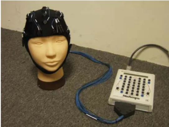
The 36 electrodes including 34 EEG/EOG channels , 2 ECG channels (bipolar connections between the right clavicle and left rib), and one 8-bit digital signal produced form VR scene were simultaneously recorded by the Scan NuAmps Express system (Compumedics Ltd., VIC, Australia) shown in Fig. 2-6. It was a high-quality 40-channel digital EEG amplifier capable of 32-bit precision sampled at 1000 Hz. Table-2 showed the specifications of the NuAmps amplifier. Before acquiring EEG data, the contact impedance between EEG electrodes and skin was calibrated to be less than 5kΩ by injecting NaCl based conductive gel. The EEG data were recorded with 16-bit quantization levels at a sampling rate of 500 Hz in this study. All EEG data were preprocessed using a low-pass filter with a cut-off frequency of 50 Hz in order to remove the power line noise and other high-frequency noise. Similarly, a high-pass filter with a cut-off frequency at 0.5 Hz was applied to remove baseline drifts.

Fig. 2-6: The picture showed the setup of the physiological recording containing the NuAmps EEG amplifier and the electrode cap.

(24)

2.3 3D Position Measurement of EEG Electrodes

The Fastrak 3D Digitizer is an accurate electromagnetic tracking system we used for localization of electrodes. With the 3D digitizer, it became possible to construct accurate anatomical/functional images from the surface measured potentials. Fastrak is controlled by software named Locator, which acquires and displays 3D position measurements for electrodes. It includes a System Electronics Unit (SEU), a power supply, three cube receivers, one stylus and one standard transmitter (as showed inFig. 2-7). Used the hardware and software necessary to generate and sense the magnetic fields, compute position and orientation for digitizing electrode locations of subject’s head.

Fig. 2-7: The picture showed the Fastrak 3D Digitizer.

Table-2: Specifications of NuAmps

Analog inputs 40 unipolar (bipolar derivations can be computed)

Sampling frequencies 125, 250, 500, 1000 Hz per channel

Input Range ±130mV

Input Impedance Not less than 80 MOhm

(25)

2.4 Experimental Design

To investigate the effect of stimulus onset asynchrony (SOA) on the behavioral performance and differences on brain activities between single- and dual- task condition in a virtual environment, we designed two tasks: unexpected car deviation, mathematical questions. We used the combinations of these two tasks to provide different distracted effects to the subjects.

We developed a VR highway environment with a monotonic scene as shown in Fig. 2-8 and eliminated all unnecessary visual stimuli. The four lanes from left to right were separated by a median strip in the VR-based scene. The distance from the left side to the right side of the road was equally divided into 256 points for outputting digital signal from WTK program, and the width of each lane and the car was 60 units and 30 units, respectively (as showed in Fig. 2-9). In the VR scene, the simulated driving speed was controlled by a scheduled program, thus subjects need not to step on paddles, to prevent large muscle activity on the throttle or brake.

Fig. 2-8: The photomicrograph showed the simulated high way scene. The

(26)

Fig. 2-9: The illustration of the high way scene. The width of highway from the left to right side was equally divided into 256 units and the width of the car was 32 units.

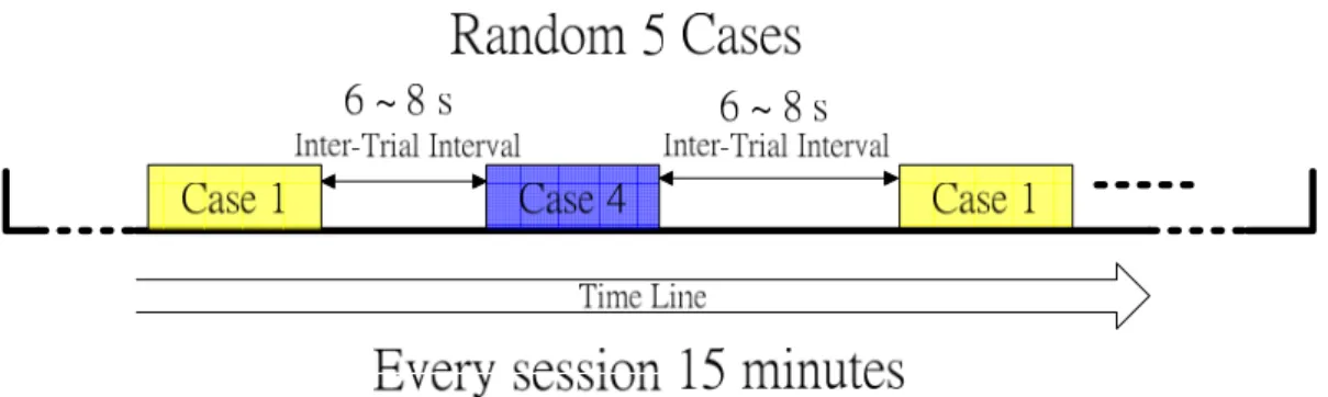
There would be four 15-minute sessions (5~10 minutes break between sessions to avoid the subject get drowsy) in one driving simulation experiment for each subject. To avoid anticipative effect for subjects the events were presented to the subjects randomly, as shown in Fig. 2-10. The inter-trial intervals were set from 6 to 8 seconds in order to avoid interaction between trial and trial. Thus a total of 100 events could be presented to the subject in each session to ensure the number of events is enough for statistical analysis.

(27)

Fig. 2-10: The illustration of the experimental paradigm. Five cases were randomly appeared and the inter-trial intervals were varied from six to eight seconds. There were four sessions (15 minutes / per session) in each experiment.

Since the main purpose of this experiment was to investigate the distracted effect in dual-task conditions. Therefore, two driving tasks were designed including the car unexpected deviation and the mathematical questions. The car would randomly drift from the middle of the road in a deviation task. When the event was occurred, subjects had to control the steering wheel to keep car in the third lane (as showed in Fig. 2-11). Response time was recorded

A

B

C

D

Response time was recorded Response time was recorded Response time was recorded Response time was recorded

A

B

C

D

Fig. 2-11: The illustration of the deviation event. (A) Vehicle moving in straight line; (B) the onset of deviation event; (C) response to the deviation and (D) vehicle back to middle lane.

(28)

Two digits addition equations were presented to the subjects in the mathematics task. The answers of the equations were already designed to present with the equations but they could be either right or wrong. The subjects were asked to press the right bottom on the steering wheel when the equation is correct, and to press the left bottom when it was wrong. The event allotment ratios were 50% and 50% for right and wrong equations, respectively.

A

B

C

D

E

Mathematical Question (before D 400ms) Case 1 400ms

Case 1 Case 2 Case 3

400ms Case 5 Case 4 Mathematical Question Case 2 Mathematical Question (after D 400ms) Case 3 Only deviation Case 5 Math Only Mathematical Question Case 4

A

B

C

D

E

Mathematical Question (before D 400ms) Case 1 400ms

Case 1 Case 2 Case 3

400ms Case 5 Case 4 Mathematical Question Case 2 Mathematical Question (after D 400ms) Case 3 Only deviation Case 5 Math Only Mathematical Question Case 4 Mathematical Question (before D 400ms) Case 1 Mathematical Question (before D 400ms) Case 1 400ms

Case 1 Case 2 Case 3

400ms Case 5 Case 4 Mathematical Question Case 2 Mathematical Question Case 2 Mathematical Question (after D 400ms) Case 3 Mathematical Question (after D 400ms) Case 3 Only deviation Case 5 Only deviation Case 5 Math Only Mathematical Question Case 4 Math Only Mathematical Question Case 4

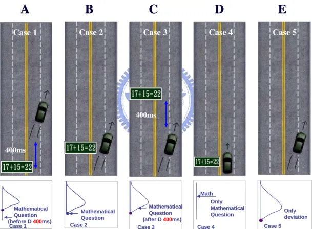
Fig. 2-12: The illustration of the relationship between the deviation onset and math occurred. (A) Case 1: math was presented at 400ms before the deviation onset. (B) Case 2: math and deviation occurred at the same time. (C) Case 3: math presented at 400ms after the deviation onset. (D) Case 4: only math presented. (E) Case 5: only deviation occurred.

The combinations of these two tasks were used to provide different distracted conditions to the subjects. Five conditions were developed to study the interaction of

(29)

the two tasks, they are: (A) math was presented at 400ms before deviation (math-400ms-deviaiton), (B) two tasks were presented at the same time (math-deviation) (C) math was presented at 400ms after deviation (deviation-400ms-math), (D) only math presented (single-math) and (E) only deviation occurred (single-deviation). The illustrations of the five conditions were shown in Fig. 2-12. A pilot study was designed to determine the time of stimulus onset asynchrony, i.e., the time interval between two tasks in case 1 and 3. Three different time values were tested including 400ms, 800ms and 1200ms. The behavioral data was collected from 8 subjects in the pilot study. The result suggested the interaction between tasks is significant with 400ms time interval. Thus, we adopted 400ms as the time of stimulus onset asynchrony.

2.5 Subjects

Eleven healthy volunteers (all males) with no history of gastrointestinal, cardiovascular, or vestibular disorders participated in the experiment of the motion-sickness study. The subjects are ages from 20 to 28 years old, with a mean of 24 years. They were requested not to smoke, drink caffeine, use drugs, or drink alcohol, all of which could influence the central and autonomic nervous system for a week prior to the main experiment.

(30)

3 III. Data Analysis

After the recording of the multi-channel EEG signals and behavior data, the data were analyzed for the study of distracted effect. The software of Statistical Package for Social Science (SPSS) was used to estimate the significant testing of behavior data. EEG epochs were extracted form the recorded EEG signals after down sampling, filter and artifact removal. We used Independent Component Analysis (ICA) [25] to separate independent brain sources. The Event Related Potential (ERP) was first used to study the EEG potential responses in time domain. The Event Related Spectral Perturbation (ERSP) technology was then applied to the ICA component signals to transfer the signal into time-frequency domain for the event-related frequency study. The stability of component activations and scalp topographies of meaningful components were finally investigated with component clustering technology.

3.1 Analysis of the Behavior Data

The response time of the tasks (the deviation and the math) was analyzed to study the behavior of the subjects in the experiments. By using one way analysis of variance (ANOVA), the significance of the behavior data were tested for every subject and the nonparametric test to study the trend of the behavior data. Fig. 3-1 showed the flowchart of analysis behavior data. First, we had to remove the outliners by using the criterion of mean±3D (mean: average the response time, D: standard deviation). Then we choose the minimal trial in all cases to make benchmark. And we used the benchmark to select randomly the same trials in other cases. Single task was baseline, and choose the minimal value as denominator. To normalize the behavior data was [Xi

(31)

／(Xmean)] (Xi: Every response time of trial, Xmean: mean response time in single case). Because several extremely large scores significantly skewed, so nonparametric analysis was used. A Friedman ANOVA was conducted to test for difference in R-values (Xi／(Xmean)) among the five in-vehicle tasks.

Fig. 3-1: The flowchart of analyzing the behavioral data. First, we removed the outliers and normalized the behavioral data by [Xi／(Xmean)] (Xi: Every response time of trial, Xmean: mean response time in single case) and then we used the Friedman test to examine the significance of R-values (Xi／(Xmean)). Finally, the Student-Newman-Keuls test was used to assess the significant within all cases.

(32)

3.2 The Procedures of EEG Data Analysis

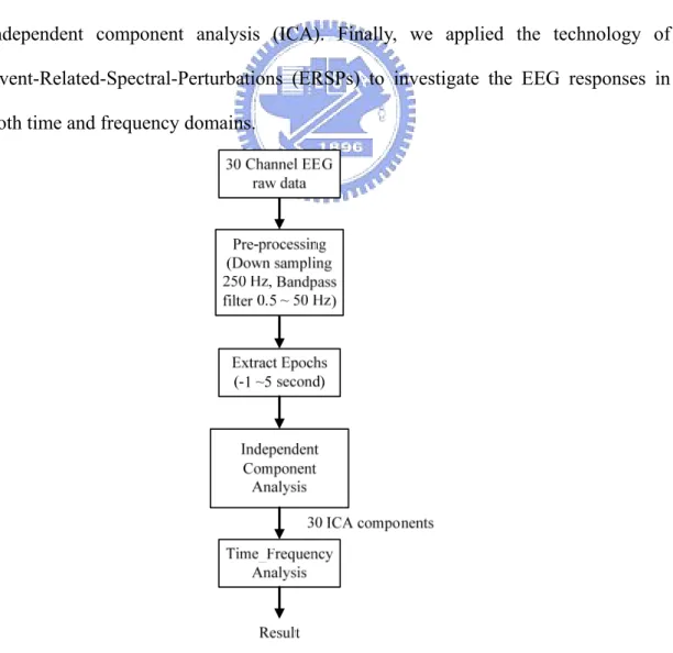
Fig. 3-2 showed the flowchart of the proposed data analysis procedure for EEG signals. The EEG data were recorded with 16-bit quantization level at a sampling rate of 500 Hz and the recording were down-sampled to sampling rate (SR) =250 Hz for the simplicity of data processing. The EEG data were then preprocessed using a simple low-pass filter with a cut-off frequency of 50 Hz to remove the line noise (60 Hz and its harmonic) and other high-frequency noise for further analysis. A simple high-pass filter with a cut-off frequency of 0.5 Hz was used to remove the DC drift. Then we extracted epochs from continuous EEG data and combine all epochs to run independent component analysis (ICA). Finally, we applied the technology of Event-Related-Spectral-Perturbations (ERSPs) to investigate the EEG responses in both time and frequency domains.

(33)

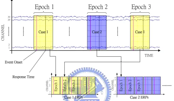
Since we had designed different cases with the combinations of the driving and the mathematic tasks, thus the EEG response related to different cases should be extracted from the original EEG signals for further analysis. The event-related potentials (ERPs) were extracted from the EEG signal as shown in Fig. 3-3.

Fig. 3-3: The illustration of the ERP analysis. The case-related ERPs were extracted from raw EEG signals. Each epoch was extracted with the duration of 1 second

before and five seconds after first event onset. The onset of first event was the

occurrence of either the math or the deviation event depended on the case was presented.

3.3 Independent Component Analysis (ICA)

In order to extract the electroencephalographic (EEG) source segregation, identification, and localization were very difficult. Because the EEG data collected from any point on human scalp induces activity generated within a large brain area. Although the conductivity between the skull and brain was different, the spatial smearing of EEG data by volume conduction did not cause significant time delay and

(34)

it suggests that the ICA algorithm is suitable for performing blind source separation on EEG data. The ICA methods were extensively applied to blind source separation problem since 1990s [26]-[33]. The reports of study [34]-[41] demonstrated that ICA was a suitable solution to solve the problem of EEG source separation, identification, and localization. They assumed that: (a) the conduction of the EEG sensors is instantaneous and linear such that the measured mixing signals are linear and the propagation delays are negligible. (b) The signal source of muscle activity, eye, and, cardiac signals are not time locked to the sources of EEG activity which is regarded as reflecting synaptic activity of cortical neurons.

) t ( ) t ( As x = (1)

Where A is a linear transform called a mixing matrix and the s are statistically i

mutually independent. The ICA model estimates a linear mapping W such that the unmixed signals u(t) are statically independent (as showed in Fig. 3-4) (The detail was in Appendix ). ) t ( ) t ( Wx u = . (2)

Fig. 3-4: Illustration of the concept of ICA process. EEG signals recorded from the brain were mixed with multiple sources [62]. By training the unmixing matrix, the mixed EEG signals were separated into independent components which may have specific meanings, and then scalp maps was plotted according to the weight of unmixing matrix.

(35)

In this study, we attempted to completely separate the twin problems of source identification and source localization by using a generally applicable ICA. Thus, the artifacts including the eye-movement (EOG), eye-blinking, heart-beating (EKG), muscle-movement (EMG), and line noises can be successfully separated from EEG activities. Fig. 3-5 showed a result of the scalp topographies of ICA weighting matrix

W corresponding to each ICA component by projecting each component onto the

surface of the scalp, which provided evidence for the components' physiological origins, e.g., eye activity was projected mainly to frontal sites, and the drowsiness-related potential was on the parietal lobe and occipital lobe [20], motor related potential will locate at left and right side of front parietal lobe, etc. We could see that most of artifacts and channel noises were effectively separated into independent components 1 and 20.

Fig. 3-5: The picture showed the typical example of scalp topography of ICA decomposition. The scalp topographies showed the ICA weighting matrix W projected to its corresponded component onto the surface of the scalp. The color bar was the amplitude of component signals.

(36)

3.4 Power Spectrum Analysis

Analysis of changes in spectral power and phase can characterize the perturbations in the oscillatory dynamics of ongoing EEG. Applying such measures to the activity time courses of separated independent component sources can avoid the confounds caused by misallocation of positive and negative potentials from different sources to the recording electrodes, and by misallocation to the recording electrodes activity that originates in various and commonly distant cortical sources. The spectral analysis for each ICA component decomposed from 30 channels of the EEG signals. The FFT processes for each ICA component data decomposed from 30 channels of the EEG signals and the processes are described as following. The sampling rate of EEG is 250Hz. The power spectrum density (PSD) of each ERP is evaluated with the spectral analysis process. The activity power spectrum of the ERP is calculated by averaging the PSDs. The ICA data power spectrum time series for each session consisted of ICA data power estimates at 50 frequencies (from 1 to 50 Hz).

The input EEG signal is x

[ ]

n . And we can consider computing X

[ ]

k by

separating x

[ ]

n into two (N/2)-point sequences consisting of the even-numbered

points in x

[ ]

n and the odd-numbered points in x

[ ]

n . 2 / ) 2 / ( 2 ) / 2 ( 2 2 N N j N j N e e W W = − π = − π = (3)

The PSDs was calculated as following equations:

[ ]

_∑

[ ]

_∑

−

[

]

= − = + + = ( /2)1 0 2 / 1 ) 2 / ( 0 2 / 2 1 2 N r rk N k N N r rk N W x r W W r x k X

[ ]

k W H

[ ]

k, G + _Nk = k =0,1,...,N −1, (4)

(37)

3.5 Event Related Spectral Perturbation Analysis

The Event Related Spectral Perturbation, or ERSP, was first proposed by Makeig [42]. ERSP, we are able to observe time-locked but not necessary phase-lock activities. It is different from the limitation of ERP.ERP must be coherent time-and-phase-locked activities. The ERSP measures average dynamic changes in amplitudes of the broad band EEG spectrum as a function of time following cognitive events.

The processing flow is shown in Fig. 3-6. The time sequence of EEG channel data or ICA activations are subject to Fast Fourier Transform (FFT) with overlapped moving windows. Spectrums in each epoch were smoothed by 3-windows (768 points) moving-average to reduce random error. Spectrums prior to event onsets are considered as baseline spectra for every trial. The mean baseline spectra were converted into dB power and subtracted from spectral power after stimulus onsets so that we can visualize spectral ‘perturbation’ from the baseline. This procedure is applied to all the epochs, the results are then averaged to yield ERSP image. The ERSP image mainly shows spectral differences after event, since the baseline spectra prior to event onsets have been removed.

After performing bootstrap analysis (usually 0.01 or 0.03 or 0.05, here we use 0.05) on ERSP, only statistically significant (p<0.05) spectral changes will be shown in the ERSP images. Non-significant time/frequency points are masked (replaced with zero). Any perturbations in frequency domain become relatively prominent.

(38)

Fig. 3-6: The illustration of procedures in ERSP analysis. FFT was applied in each window with 256 samples, and there was 244-sample overlap of two adjacent windows. The time-dependent ERSP image was composed of the spectra of each window, and smoothed by 3-window moving average. In the final step, the significant parts of ERSP image were extracted by using bootstrap method. The pink dashed lines: the first event onset. The blue dashed lines: the averaged reaction time to the deviation. The red dashed lines: the averaged response time to math. The black dashed lines: averaged response time for the car returning to the third lane. Color bars showed the magnitude of ERSPs.

(39)

3.6 Component Clustering

To study the cross-subject component stability of ICA decomposition, components from multiple subjects were clustered based on their spatial distributions and EEG characteristics. But, components from different subjects thus may differ in many ways such as scalp maps, power spectra, ERPs and ERSPs. [43] [44] [45] attempted to solve this problem by calculating the similarities (distance) among different independent components. Components from multiple subjects were clustered in terms of their scalp maps and activation power spectra. Individual component clusters were characterized by their mean cluster map and activity spectrum. This method was also known as component clustering.

In this study, we attempt to completely components cluster. We used the K-means algorithm (EEGLAB 4.3) to analyze (as shown in Fig. 3-7). To cluster these components into small number (for instance, 10) of groups, one approach is to apply K-means on their scalp map and power spectral. In practice, we could hardly achieve such clean clusters if we relied entirely on K-means to classify components, since less then half of components were meaningful after ICA decomposition, others were usually account for noises. These components might confuse K-means algorithm and reduce the consistency of each clusters. Another problem arose from combining scalp map and power spectral information for K-means classification. It remained an open question how to weight the spatial information (scalp maps) and source activity, accounted for by power spectra in the K-means clustering. Therefore, we selected stable components which were classified iteration by K-means algorithm into 16 clusters in terms of component scalp maps (EEG.icawinv). Then we grouped 16 clusters into 7 significant clusters and discarded some non-significant clusters

(40)

manually based on power spectra of the components. The resultant clusters are named according to the source locations of components (as shown in Fig. 3-8).

Components from 1 subject

Com

ponent Pool

C

omponent

Clusters

Components from 1 subject

Com

ponent Pool

C

omponent

Clusters

Fig. 3-7: The flowchart of component clustering by using K-means algorithm. Components from 11 subjects were classified into several significant clusters according to their K-means.

Fig. 3-8: The typical example of the component clustering result. The mean of scalp map was averaged across 11 subjects.

(41)

4 IV. Results

The EEG signals collected from 11 subjects were analyzed for the study of distraction. Each experiment included 4 sessions and each session lasted 15 minutes. Every session presented five cases randomly (designed with different time intervals between tasks). The influence of stimulus onset asynchrony in the subjects’ behavior performance was studied in the first section. Then we characterized changes of dynamic brain activities from the independent component clusters and the power spectrum and the event-related spectral perturbations (ERSPs) under different cases. The following paragraphs showed detailed results.

4.1 Behavior Performance

The response time of the tasks (the deviation and the math) was collected to study behavior of the subjects in the experiments. The outliers were first removed from the 11 subjects’ behavior data. By using one way ANOVA, the significance of the behavior data were tested for every subject. The testing results were showed in Fig. 4-1. The response time to deviation was given in Fig. 4-1(A). The blue bars were in the figures represented the case of math-400ms-deviation (case-1), the light blue bars were represented the case of math-deviation (case-2), the yellow bars were represented the case of deviation-400ms-math (case-3), and the red bars were represented the case of single-deviation (case-5).

The response time to deviation in case-5 (single deviation) was significantly larger than that in the case-1 (math present 400 ms before deviation) for most of the subjects (8 out of 11). The response time to deviation in case-5 (single deviation) was

(42)

significantly larger than that in the case-2 (two tasks present at the same time) for four subjects. And, the response time to deviation in case-5 (single deviation) was significantly larger than that in the case-3 (deviation present 400 ms before math) for only one subject. These results were shown in Fig. 4-1(A). This meant it take longer time for the subjects to reply to the driving task in single deviation case. Because when the deviation task appeared in the case-1 subjects were in order to continuously resolve the mathematical equations, they had to firstly and rapidly response to the deviation task to avoid hitting the wall.

The Responses to Deviation

Time (ms)