VOLUME 15, NUMBER 3 HVAC&R RESEARCH MAY 2009
461
Performance Analysis and Optimized Design of
Backward-Curved Airfoil Centrifugal Blowers
Chen-Kang Huang, PhD
Mu-En Hsieh
Received October 21, 2008; February 15, 2009
In this study, backward-curved airfoil centrifugal blowers were numerically simulated and com-pared with experimentally measured data. Simulation settings and boundary conditions are stated, and the measurements follow ANSI/AMCA Standard 210-07/ANSI/ASHRAE Standard 51-07, Laboratory Methods of Testing Fans for Certified Aerodynamic Performance Rating (AMCA/ASHRAE 2007). Comparing simulation results with measured data, it was found that the deviation of the static pressure curve at each specified flow rate was within 4.8% and the deviation of the efficiency curve was within 15.1%. After the simulation scheme was proven valid, the effects of blade angle, blade number, tongue length, and scroll contour were dis-cussed. Several parameter changes are suggested based on these simulations. An optimized design is presented with a 7.9% improvement in static pressure and a 1.5% improvement in effi-ciency. Overall, the whole process simulates backward-curved airfoil centrifugal blowers effec-tively and is a powerful design tool for blower development and improvement.
INTRODUCTION
A blower is a gap pump that is capable of providing moderate to high pressure rise and flow rate. Blowers are utilized widely in all kinds of engineering applications, such as building venti-lation, air-supply in processes, and consumer electronics. There are three main types of blowers used for moving air: axial, centrifugal, and mixed flow. Among the three main types, centrifu-gal blowers (shown in Figure 1) are commonly applied to general heating, ventilating, and air-conditioning applications. They are usually only applied to larger systems, which may be low-, medium-, or high-pressure applications, and large, clean-air industrial operations for sig-nificant energy saving. Depending on the blade design, centrifugal blowers can be categorized into forward-curved, backward-curved, radial, and airfoil types. While the first three types are relatively easy to manufacture, centrifugal blowers with airfoil type blades exhibit the following characteristics (ASHRAE 1996; Cengel and Cimbala 2006):
• highest efficiency of all centrifugal blower designs
• blade of airfoil contour curved away from direction of rotation • air leaves impeller at velocity less than tip speed
• scroll-type design for efficient conversion of dynamic pressure to static pressure • maximum efficiency requires close clearance and alignment between wheel and inlet
• highest efficiencies occur at 50% to 60% of wide open volume; the pressure characteristics around the peak efficiency point are still efficient
• power reaches maximum near peak efficiency and becomes lower, or self-limiting, toward free delivery
Chen-Kang Huang is an assistant professor in the Department of Bio-Industrial Mechatronics Engineering, National
Taiwan University, Taipei, Taiwan. Mu-En Hsieh is a graduate student in the Institute of Mechatronic Engineering, Na-tional Taipei University of Technology, Taipei, Taiwan.
Including the centrifugal blowers we focus on in this study, blowers can be analyzed theoreti-cally, then some basic performance characteristics can be derived and calculated from simple equations (Logan 1993; Fox and McDonald 1998). The horsepower, which is the useful power actually delivered to the fluid, can be written as Equation 1:
(1) where ρ is the fluid density, g is the gravitational acceleration constant, Q is the volume flow rate, and H is the net head of the blower. The external power supplied to the pump is the brake horsepower (bhp). Equation 2 provides the definition of brake horsepower:
(2) where ω is the rotational speed of the shaft and Tshaft is the torque supplied to the shaft. The blower efficiency, usually abbreviated as ηpump, then can be defined as follows:
(3)
The idealized velocity tangential and normal components are shown in Figure 2. The fluid is assumed to enter the impeller wheel at radius r1 with uniform absolute velocity V1 and to leave the impeller wheel at radius r2 with uniform absolute velocity V2. The rate of work done on an impeller wheel can be written as
, (4)
where U is the tangential speed of the impeller wheel at radius r and is the mass flow rate. The head added to the flow, which is the dimension of length, can be written as
. (5)
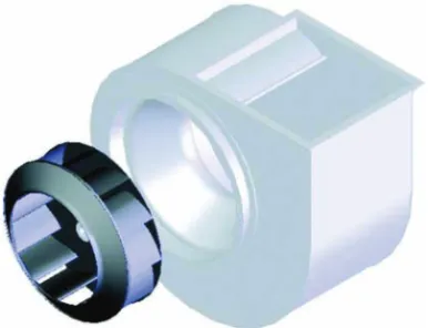
Figure 1. Explosion view of a typical centrifugal blower.
W·horsepower = ρ g Q H⋅ ⋅ ⋅ bhp = W·shaft = ω T⋅ shaft ηpump W·horsepower bhp --- ρ g Q H⋅ ⋅ ⋅ ω T⋅ shaft ---= = bhp ω T⋅ shaft ω r2 Vt 2–r1⋅Vt1 ⋅ ( ) ⋅ ⋅m· U2 Vt 2–U1⋅Vt1 ⋅ ( ) m·⋅ = = = m· H bhp m· g⋅ --- 1 g --- U2 Vt 2–U1⋅Vt1 ⋅ ( ) = =
If the fluid enters the impeller with purely radial absolute velocity, . The increase in head becomes
. (6)
Observing the exit velocity triangle in Figure 2, it can be found that
. (7)
Then
, (8)
where represents the ideal flow rate for an impeller of width w. The theoret-ical derivations in Equations 1–8 estimate the performance of ideal blowers. But, these equa-tions cannot investigate several effects on actual blower performance, such as number of blades and scroll contour. More powerful tools are necessary to take more design parameters into account to better estimate the blower performance and facilitate the design process.
Computational fluid dynamics (CFD) packages have progressed to the point where they can produce accurate predictions for thermal and fluid applications (Gonzalez et al. 2002; Kim and Seo 2004; Medvitz et al. 2002; Tsai and Wu 2007; Velarde-Suarez et al. 2001). Subhash and Majumder (2007) used FLUENT (Fluent 2005a) to solve a large eddy simulation (LES) model for the film cooling problem. After the time-dependent analysis, they obtained the temperature, pressure, and velocity distributions. Numerous researchers have used CFD simulations to study turbo-machinery. Calvert and Ginder (1999) studied transonic fans and compressors. In their
Figure 2. Velocity vector diagram of impeller wheel in a backward-curved blower.
vt 1 = 0 H U2 Vt 2 ⋅ g ---= Vt 2 = U2–Vn2cot( )β2 H U2 2 U 2 – ⋅Vn2cot( )β2 g --- U2 2 g --- U2⋅cot( )β2 2π r⋅ 2⋅ ⋅w g ---Q – = = Q = 2π r⋅ 2⋅ ⋅w Vn2
study, the evolution of transonic compressor designs and methods was outlined, followed by more detailed descriptions of current compressor configurations and requirements and modern aerodynamic design methods and philosophies. Detailed quasi-dimensional and three-dimensional computational fluid dynamics analyses were employed to refine the design. Lin and Huang (2002) numerically simulated the internal flow for a forward-curved centrifugal fan used in notebook PC cooling. In their study, an integral solution, including design powered by CFD, prototype manufacturing, and experiment verification, was presented. With results from CFD simulation, they concluded the optimum inlet angle design to smooth the airflow around the inlet. Thakur et al. (2002) used a CFD-based computational tool to analyze fluid flow in a cen-trifugal blower. Global quantities such as static pressure rise, horsepower, and static efficiency were compared between calculation results and measured data. They concluded that the overall CFD predictions are satisfactory. Yu et al. (2005) carried out numerical simulation for a whole centrifugal fan and derived the optimum design. A sample fan was manufactured and tested, and the numerical prediction agrees well with the tested data. Katsumi and Tetsouo (1999) investi-gated the form of volute tongue that affects the characteristics of a centrifugal blower. They pre-sented visualized experiments and numerical calculations for the tongue shape of three types and clarified the flow characteristics of the flow near the tongue in a centrifugal blower. It was con-cluded that the behavior of the flow near the tongue agrees with that obtained by flow visualiza-tion experiments and that the stagnavisualiza-tion point moves around the tongue when changing the mass flow. Dilin et al. (1998) presented a detailed experimental study of the performance of two radial-flow fan volutes. Their research included a volute with a full tongue and the same volute with the tongue cut back to allow flow recirculation. A computational model, using the k–ε tur-bulence model, was used to predict the internal flow of both volutes. The performance of the volutes was discussed, and the CFD analysis was used to recommend design improvements for the volute.
NUMERICAL SIMULATION
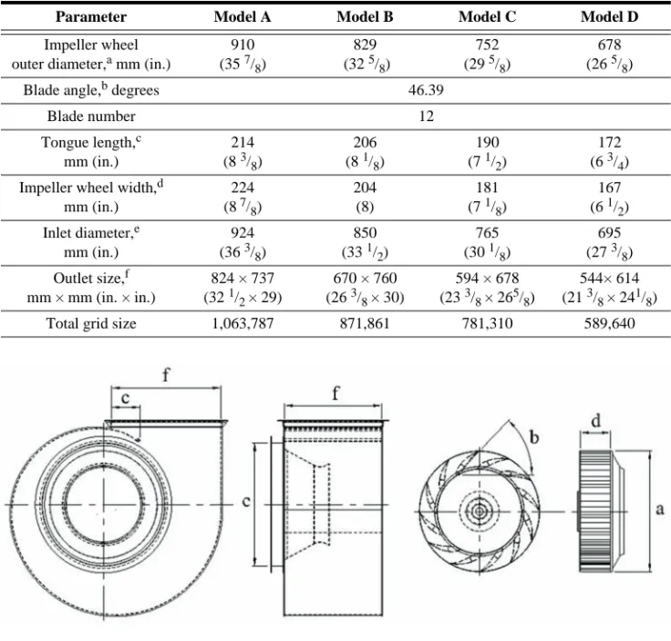
In this study, the commercial CFD package FLUENT is used to simulate four backward-curved airfoil centrifugal blowers. The primary parameters of the four blowers are listed in Table 1. FLUENT solves the Navier-Stokes equation using the finite volume method (FVM), which has been applied widely in fluid mechanics and engineering applications. It has been shown that the FLUENT quasi-steady simulation can be used to predict blower performance. The simulation results are compared with the measured results to verify the validity. This sec-tion states code verificasec-tion, grid system generasec-tion, and boundary condisec-tion settings of this study. For more details about the simulation scheme, please refer to the study by Hsieh (2007).
Model Construction
For this study, the three-dimensional blower models were first created in computer-aided design (CAD) software (as shown in Figure 1) and exported into STEP files (ISO 2002). The STEP files were then imported into GAMBIT (Fluent 2005b), the mesh generator. In GAMBIT, model construction and split were processed. The fluid volume was split into a rotating fluid volume, a scroll volume, an inlet cone volume, and an inlet/outlet duct volume. The inlet and outlet ducts were intentionally set to simulate the actual measuring situation and to provide bet-ter boundary conditions for simulations. In this study, the length of the inlet duct was set to 10 times the diameter of the inlet duct and the outlet duct length was set to 15 times the diameter of the outlet duct. Consequently, the flow was assumed fully developed when leaving the inlet and outlet ducts. The impeller wheel volume was defined as a rotating reference frame with constant rotational speed, and other blocks were defined in a stationary frame. This setup is referred to as a “frozen rotor” model in other literature.
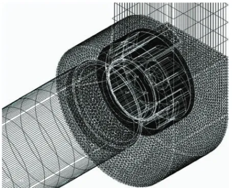
Grid Generation
According to official GAMBIT technical documents (Fluent 2005b), the system automati-cally chooses the most suitable elements for complex geometry. The rotating fluid and scroll volumes were defined by tetrahedral/hybrid elements, and hex/wedge elements were selected for the inlet cone and inlet/outlet duct volumes. A typical grid system is shown in Figure 3. Grid independency tests were performed for each model discussed in this study. To ensure the grid system was appropriate for high-speed flow, free delivery was selected to be the operating con-dition for the grid independency test. The inlet flow rate was then given as the inlet boundary condition. The outlet boundary condition was set as static pressure equal to the atmospheric pressure. If the difference of the outlet flow rate caused by further increasing grid size was below 1%, the grid size was taken to perform all simulations for the model. The records of grid independency testing for Model A are shown in Figure 4. For each model, the same process and judging philosophy were applied to choose the suitable grid size. The grid sizes for the four models discussed in this study are listed in the row titled “Total grid size” in Table 1.
Table 1. Primary Parameters of Blowers Discussed in This Study*
Parameter Model A Model B Model C Model D
Impeller wheel outer diameter,a mm (in.)
910 (35 7/8) 829 (32 5/8) 752 (29 5/8) 678 (26 5/8)
Blade angle,b degrees 46.39
Blade number 12 Tongue length,c mm (in.) 214 (8 3/8) 206 (8 1/8) 190 (7 1/2) 172 (6 3/4) Impeller wheel width,d
mm (in.) 224 (8 7/8) 204 (8) 181 (7 1/8) 167 (6 1/2) Inlet diameter,e mm (in.) 924 (36 3/8) 850 (33 1/2) 765 (30 1/8) 695 (27 3/8) Outlet size,f mm × mm (in. × in.) 824 × 737 (32 1/2 × 29) 670 × 760 (26 3/8 × 30) 594 × 678 (23 3/8 × 265/8) 544× 614 (21 3/8 × 241/8) Total grid size 1,063,787 871,861 781,310 589,640
Assumptions and Numerical Model
In this study, several assumptions were made to facilitate the simulations: 1. incompressible flow
2. no-slip boundary condition 3. gravity effects are negligible
4. fluid properties are not functions of temperature
Turbulence modeling is a key issue in most CFD simulations. Most engineering applications are turbulent and require a turbulence model to facilitate the calculation. In the past decades, algebraic models, one- and two-equation models, non-linear eddy viscosity models, algebraic stress models, Reynolds stress transport models, detached eddy simulations, LESs, and direct numerical simulations have been proposed to model the random nature. Among these models,
Figure 3. Grid system.
Figure 4. Grid independency tests for Model A: a) SI units, b) I-P units.
two-equation turbulence models are one of the most common turbulence models. Two-equation models include two extra transport equations to represent the turbulent properties of the flow. This allows a two-equation model to account for effects of convection and diffusion of turbulent energy. One of the transported variables is the turbulent kinetic energy, k, which determines the energy in the turbulence. The second transported variable is the turbulent dissipation, ε, which can be thought of as the variable that determines the length scale of the turbulence. The k-ε model has become one of the industry standard models and is commonly used for most types of engineering problems. In this study, the standard k-ε model with standard wall functions was chosen in the Viscous Model menu of the FLUENT solver. The SIMPLE numerical algorithm was used (Fluent 2005a). In addition, the pressure parameter was discretized by second-order central difference, and the parameters of k and ε were discretized by second-order upwind scheme.
Boundary Conditions
The boundary conditions for blowers discussed in this study consisted of inlet, outlet, and impeller wheel boundary conditions. At the beginning of this study, the total pressure at the entrance of the inlet was given as the inlet boundary condition. It was found that this method encountered some difficulties in converging in the low flow rate region of the performance curve. The inlet flow rate was then given as the inlet boundary condition. The outlet boundary condition was set as static pressure equal to the atmospheric pressure. Motion wall type was selected to be the impeller wheel boundary condition, and the relative velocity between the impeller wheel and the rotational volume was assumed to be zero.
Converging Criteria
While the convergence criteria were usually set at 10–5 for the residuals of all quantities, it was observed that the residuals remained around 10–2 for high pressure/low flow rate condi-tions. For some other cases in this study, the numerical results could not converge to 10–5 but changed periodically within a range around 10–3 to 10–4. This has also been observed by other researchers (Yu et al. 2005), and the unsteady nature in centrifugal fans could be one of the rea-sons. Eventually, the convergence criteria were still set at 10–5, but the iterations were intention-ally stopped if periodical phenomenon occurred. The actual achieved convergence levels (residuals of continuity) are listed in Table 2.
The higher convergence levels imply that the result may be slightly away from the exact one and may lead to imprecise simulation results. It should be noted that the convergence level is higher around free delivery and shutoff conditions. Fortunately, the two extreme conditions are not usually utilized in engineering applications. Comparing Model A to Model D in Table 2, it can be found that the convergence level of the smaller blower (Model D) is higher. This trend confirms the simulation results presented in the Results and Discussion section of this paper.
Table 2. Continuity Convergence Levels of Blowers Discussed in This Study
Model Flow Rate
Low High
A 1.45×10⁻³ 3.52×10⁻⁵ 1.75×10⁻³ 1.25×10⁻³ 1.3×10⁻⁵ 1.07×10⁻⁵ 9.98×10⁻⁶ 7.21×10⁻⁶ 6.26×10⁻⁴ B 4.44×10⁻³ 6.56×10⁻⁴ 3.75×10⁻³ 5.56×10⁻⁵ 3.62×10⁻⁵ 2.62×10⁻⁵ 1.88×10⁻⁴ 6.03×10⁻⁴ 8.17×10⁻⁴ C 1.94×10⁻³ 3.44×10⁻⁴ 1.50×10⁻³ 8.27×10⁻⁴ 2.0×10⁻⁵ 1.97×10⁻⁵ 9.12×10⁻⁶ 7.72×10⁻⁶ 2.16×10⁻³ D 1.23×10⁻³ 2.11×10⁻⁴ 9.55×10⁻⁴ 2.5×10⁻³ 3.84×10⁻⁵ 1.52×10⁻⁵ 2.0×10⁻⁴ 5.49×10⁻⁴ 1.49×10⁻³
The shaft power was calculated using Equation 2. FLUENT can compute and report moments about a specified center for selected wall zones. The total moment vector about a specified cen-ter is computed by summing the cross products of the pressure and viscous force vectors for each face with the corresponding moment vector, which is the vector from the specified moment center to the force origin. Eventually, the efficiency can be calculated using Equation 3.
While the acoustic performance of the blower is important as well, its corresponding simula-tion is tougher and more time consuming. The CFD simulasimula-tion process has to begin with a steady flow analysis, which includes all tasks described in this section. Thereafter, an unsteady calculation is then performed using a sliding mesh. During the unsteady calculation, oscillating values of pressure and velocity at several monitoring points located behind the rotating impeller wheel can be acquired. The periodic time histories of the pressure and the velocity values can be used to indicate when the unsteady flow calculation is fully developed. Only after this stage has been reached is an unsteady acoustic analysis performed. For each case, the time needed to per-form an unsteady acoustic analysis can be weeks using a state-of-the-art system. Therefore, the acoustic analysis has not yet been performed in this research at this point.
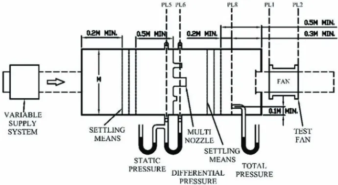
EXPERIMENTAL VALIDATION
In this study, four blowers were tested in the Ventilation Systems Laboratory at the Industrial Technology Research Institute, Hsin-Chu, Taiwan. The laboratory possesses the facility for fan or blower performance tests in accordance with the requirements of ANSI/AMCA Standard 210-07/ANSI/ASHRAE Standard 51-07, Laboratory Methods of Testing Fans for Certified Aerodynamic Performance Rating (AMCA/ASHRAE 2007). The apparatus complied with AMCA 120/ASHRAE 51 (Figure 5). The wind tunnel is used to determine the aerodynamic per-formance of a fan or blower. The main components include the main structure (rectangle or round section is most seen), auxiliary supply system, grid, settling means, and multiple nozzles to vary the airflow rate. The apparatus performs one of the most common procedures for devel-oping the characteristics of a blower tested from shutoff conditions to nearly free delivery condi-tions, while various flow restrictions are placed on the opening of the inlet duct to simulate
various conditions on the blower. In some cases, measurements are done by restrictions placed on the outlet duct. For those cases, the static pressure at the inlet is lower than the atmospheric pressure. The performance curves are obtained from sufficient points defined by the correspond-ing flow rate and static pressure rise. The static pressure rise, flow rate, and shaft power of the blower are obtained by measurement. The total pressure rise is obtained by the static pressure plus the averaged dynamic pressure head.
In this study, the uncertainty in the flow rate and the pressure measurements is ±2.5%. More-over, the fan input power obtained is within ±5%. Outlet velocity uniformity results obtained are not different by more than ±7.5%. Velocity profile results obtained are not different by more than ±7.5%. The rotational speed variation during the test is controlled within ±1%. Twenty-four measurements were made to derive the velocity profile and the corresponding flow rate.
When performing the blower tests, long ducts that are at least ten times the tube diameter are installed at the suction and discharge sides of the testing blower. As described previously, the installation of long inlet and outlet ducts was considered in our simulation.
RESULTS AND DISCUSSION
For each model discussed in this study, the simulation and measured results are shown in two plots, where the x-axes are both the input flow rate and the y-axes are static pressure and effi-ciency. Error bars for measurement data represent the measurement uncertainty acquired from the test facility. Error bars for simulation data are from additional simulations with maximum allowable rotational speeds when the measurement uncertainty is considered. However, the error bars in Figure 10 are not from rotational speed variation since the results of two rotational speeds are shown; those error bars are from additional simulations with maximum allowable geometry variation, which is ±2% enlargement or shrinkage on all parts.
From the manufacturer’s point of view, the four models belong to the same family (with the same blade angle and blade number) and are mainly different in size. The blower size decreases from Model A to D. For Model C, two rotational speeds were simulated to check the effective-ness of the simulation at different rotational speeds. For the other three models, only one rota-tional speed was simulated. By observing the results from all four models, the effects of blower size on simulation effectiveness can be found. By comparing the Model C results from two rota-tional speeds, the effects of blower rotarota-tional speed on simulation effectiveness can be found.
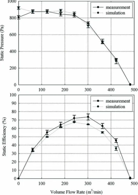
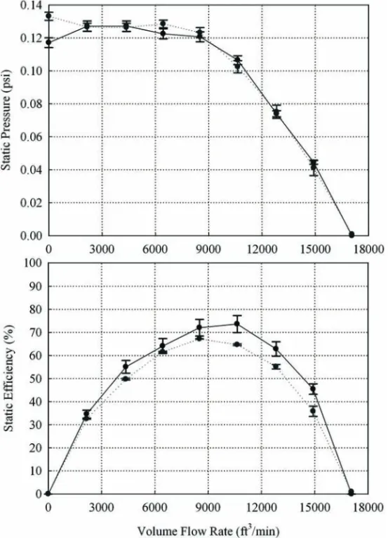
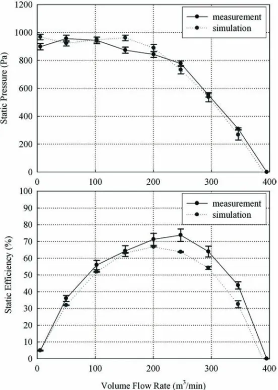
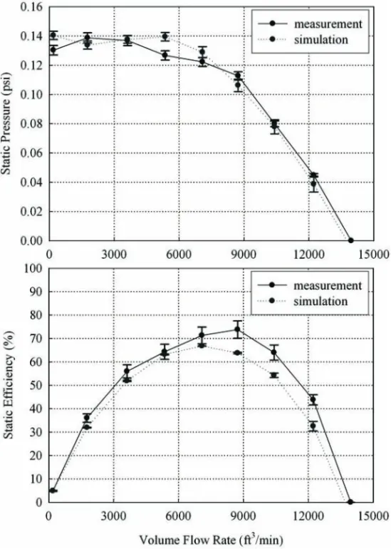
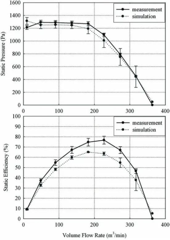
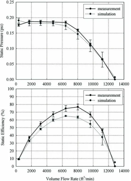
Including simulation and measurement data, the performance curves of the four tested blow-ers are shown in Figures 6 through 9. It can be found that the simulation data agree well with the measured results. The R-squared values were calculated and are listed in Table 3. R-squared measures how successful the simulation is in explaining the variation of the measured data. For all four models, the R-squared values of static pressure are close to 1, indicating that a greater proportion of variance is accounted for by the simulation. On the other hand, the efficiency results are not as good as the static pressure ones; potential reasons for the imprecise efficiency simulation will be discussed later. Furthermore, the root mean square error (RMSE) values between simulation and measurement (also listed in Table 3) for each model are calculated to examine the closeness of the two curves. RMSE results imply that the simulation scheme pro-duces more precise results for larger blowers. Comparing the two rotational speeds of Model C (shown in Figure 10), it can be found that the simulation results deviate more at higher rotational speed. From the error bars in Figure 10, it can be found that the effects of geometry variation are greater when operating conditions are closer to the free delivery condition.
Overall, the results indicate that the simulation scheme predicts the blower performance pretty well. The simulated static pressures are within 4.8% of the measured data. The efficiency curves are relatively deviated and are within 15.1% of the measured data. Since the efficiency
Figure 6a. Measured and simulated performance and efficiency curves of Model A oper-ating at 882% ± 1% rpm (SI units).
Figure 6b. Measured and simulated performance and efficiency curves of Model A oper-ating at 882% ± 1% rpm (I-P units).
Figure 7a. Measured and simulated performance and efficiency curves of Model B oper-ating at 980% ± 1% rpm (SI units).
Figure 7b. Measured and simulated performance and efficiency curves of Model B oper-ating at 980% ± 1% rpm (I-P units).
Figure 8a. Measured and simulated performance and efficiency curves of Model C oper-ating at 1280% ± 1% rpm (SI units).
Figure 8b. Measured and simulated performance and efficiency curves of Model C oper-ating at 1280% ± 1% rpm (I-P units).
Figure 9a. Measured and simulated performance and efficiency curves of Model D oper-ating at 1280% ± 1% rpm (SI units).
Figure 9b. Measured and simulated performance and efficiency curves of Model D oper-ating at 1280% ± 1% rpm (I-P units).
calculation is based on Equation 3, it is believed that the imprecise torque calculation may be the main cause of the error. The moment calculation consists of pressure and viscous parts, and the viscous part can be questionable. The viscous model may perform imprecise viscous calculation and lead to the moment calculation deviation. Since the simulation is based on a rotating fluid block, the weight of the impeller wheel is not included to perform the moment calculation. This may also contribute the imprecise calculation.
It is also concluded that the current simulation scheme does a better job for blowers with a larger impeller wheel. For the same blower, the simulation is more precise for lower rotational speed. Based on the comparative results from the four models, it is believed the simulation scheme, including model construction in CAD, mesh generation, numerical simulation, and post-processing, is successful. The process is able to predict the performance for future models without requiring significant amounts of time and expense on prototypes and field tests. After the simulation scheme was shown to be reliable, the process was utilized as a tool to discuss the effects of some blower design parameters.
Effects of Blade Angle
The effects of blade angle can be estimated quantitatively from the theoretical equations. From Equation 8, it can be found that the added head is a function of β2. When the blade angle increases, then β2 increases. From 40° to 50°, cotangent is a decreasing function. Consequently, the increase of β2 will lead to the decrease of cot(β2) and the increase of added head. This implies that, for the same flow rate, the added head increases when β2 increases.
In this simulation, we took 49.39° and 43.39° to perform the simulation and compared results with the original design of 46.49°. The schematic of impeller wheels with different blade angles is shown in Figure 11. Comparative results are listed in Sets A and B of Table 4. It was found that a 49.39° blade angle exhibited much higher static pressure rise and slight efficiency decrease. We decided the 49.39° was a favored blade angle, especially for applications where a high static pressure rise is needed.
Effects of Blade Number
The number of blades directly affects the required material and manufacturing costs. Within close performance, it is preferable to have as few blades as possible. Since a blade number of 8 to 12 is usually recommended in the literature, blade numbers of 8, 10, and 14 were simulated to compare with the blade number of 12. The schematic of impeller wheels with different blade numbers is shown in Figure 12. From Sets C, D, and E in Table 4, it can be found that the blade number of 10 exhibits a slight decrease in static pressure and flow rate. From a manufacturing cost point of view, decreasing the number of blades from 12 to 10 is a favored change.
Table 3. R-Squared and RMSE between Measured and Simulated Static Pressure and Efficiency
Model/rpm Static Pressure Efficiency
R-Squared RMSE, Pa (psi) R-Squared RMSE, %
Model A/882 1.11 41.74 (6.054×10⁻³) 0.85 5.73
Model B/980 1.17 48.31 (7.007×10⁻³) 0.91 6.70
Model C/1280 0.92 59.69 (8.657×10⁻³) 0.65 8.46
Model C/1470 0.95 74.42 (1.079×10⁻²) 0.64 9.17
Figure 10a. Measured and simulated performance and efficiency curves of Model C oper-ating at 1280 and 1470 rpm (SI units).
Figure 10b. Measured and simulated performance and efficiency curves of Model C operating at 1280 and 1470 rpm (I-P units).
Table 4. Parameter Changes and the Corresponding Effects on the Blower Performance Set A B C D E F G Parameter change Blade angle = 49.39° Blade angle = 43.39° Blade number = 14 Blade number = 10 Blade number = 8 Tongue length Scroll contour by Bleier Static pressure* +20.39% –14.31% –0.69% –2.98% –11.67% +0.96% +4.19% Efficiency* +0.75% –2.46% –1.13% –1.35% –3.96% +0.28% +2.02% Peak efficiency –2.18% –0.03% +0.26% –1.00% –3.56% –0.34% +0.84% A favored parameter change? Y N N Y N Y Y
*Flow rate at inlet = 357.4 m3/min (12620 ft3/min), the flow rate where approximately 50% of the maximum static
pres-sure rise occurs.
Figure 11. Schematic of impeller wheels with different blade angles.
Effects of Tongue Length
The blower tongue is a short wall spirally extended from the scroll to the outer periphery of the rotor. Intuitively, the tongue is installed to avoid back flow from the outlet region. Research-ers have shown that tongue form affects the blower performance (Katsumi and Tetsuo 1999). It would also be interesting to estimate the effects on the overall performance when we adjust the length of the tongue. In this study, a half-long tongue was set to compare with the original full-length tongue. The schematic of scrolls with different tongue lengths is shown in Figure 13. Results from the short tongue length are listed in Set F of Table 4.
The results show that cutting the tongue length to one half slightly decreases the maximum efficiency but increases both efficiency and static pressure with a flow rate equal to 357.4 m3/min (12620 ft3/min). Consequently, a half-long tongue is considered a favored change.
Effects of Scroll Contour
In fan/blower design handbooks, there are several recommended scroll contours and various methods presented to obtain those contours. In this study, we followed the contour described in the literature (Bleier 1998) and redesigned the scroll contour for Model A. The design criteria follow.
• The scroll shape is approximated by three circular sections whose radii are 71.2%, 83.7%, and 96.2% of the impeller wheel diameter.
• The centers of the three sections are located off the center lines by intervals of 6.25% of the wheel diameter.
• The height of the outlet is 112% the impeller wheel diameter.
• The one-piece cutoff continues the curvature of the scroll and protrudes into the housing outlet by 20% to 30% of the outlet height. The cutoff clearance is 5% to 10% of the wheel diameter.
In Figure 14, the new contour is shown to the right of the original one. A schematic for Ble-ier’s (1998) parameters to construct the contour is also shown. Comparing the original and new scroll contours, the major difference is the length of the outlet and the design of the tongue.
The simulated results for the new contour are listed in Set G of Table 4. It is found that the new contour increases static pressure and efficiency with a flow rate equal to 357.4 m3/min (12620 ft3/min) as well as peak efficiency. It can be concluded that a contour following Bleier’s
Figure 13. Schematic of scroll with different tongue lengths (left: original; right: one-half of original).
Figure 14. Scroll contours (top left: original; top-right: modified based on Bleier’s (1998) recommendation—dashed enclosures highlight the major differences; bottom: schematic of Bleier’s parameters to construct the contour).
(1998) recommendation indeed improves the blower performance and can be considered a favored parameter change.
OPTIMIZED DESIGN
The effects of blade angle, blade number, tongue length, and scroll contour have been dis-cussed in the previous section are organized in Table 4. It should be noticed that the recommen-dations in Table 4 are based on cost/performance and the balance between higher static pressure rise, higher flow rate, and lower manufacturing cost. Based on the conclusions recorded in Table 4, the virtual Model A+ was modified from Model A with all favored parameter changes: A, D, and G.
The schematic of the impeller wheel and the scroll for virtual Model A+ is shown in Figure 15. The virtual Model A+ was first constructed in CAD and then imported into GAMBIT and FLUENT. Simulations were performed to produce performance data. Comparing simulated results between Models A and A+, the performance and efficiency curves are shown in Figure 16. It can be found that the performance curve for the optimized model moves upward-right, meaning higher static pressure and volume flow rate. The peak efficiency for the optimized model decreases about 5%. However, the efficiency increases significantly in the high flow rate region. Taking an average from all operating points, the optimized design exhibits a 7.9% improvement in static pressure and a 1.5% improvement in efficiency. The results show that the optimization is successful. The conclusive favored parameter changes are a valuable ref-erence for future blower designs.
CONCLUSION
In this study, backward-curved airfoil centrifugal blowers were numerically simulated and analyzed. The results from numerical simulations and measurements were compared to verify the validity of numerical simulation.
The numerical simulations of centrifugal blowers are shown to be effective. The deviations of the performance curves and the efficiency curves are within 4.8% and 15.1%, respectively. The effects of blade angle, blade number, tongue length, and scroll contour were numerically stud-ied. Some favored parameter changes were determined and utilized to redesign one of the
blowers. The optimized model indeed exhibits a better value of cost/performance. This further shows that the presented simulation scheme is successful and that the favored parameter changes are a good reference for future blower designs.
ACKNOWLEDGMENT
The authors gratefully acknowledge the support from National Science Council (NSC) of Tai-wan (Grant number NSC 94-2622-E-027-045-CC3).
NOMENCLATURE
bhp = brake horsepower, W (Btu/h)
g = acceleration of gravity, m/s2 (ft/s2)
H = net head, m (ft)
= mass flow rate, kg/s (lb/s)
Q = volume flow rate, m3/s (ft3/m)
r = radius, m (ft)
T = torque, N⋅m (ft⋅lbf)
U = tangential speed, m/s (ft/s)
V = velocity, m/s (ft/s)
w = impeller wheel width, m(ft)
W = work, J (Btu)
Greek Symbols
β = blade angle, ° η = efficiency, %
ρ = density, kg/m3 (lb/ft3) ω = rotational speed, rad/s
Subscripts
1 = inner periphery of impeller wheel 2 = outer periphery of impeller wheel
t = tangential component
n = normal component
REFERENCES
ASHRAE. 1996. 1996 ASHRAE Handbook—Air-Conditioning Systems and Equipment. Atlanta: American Society of Heating, Refrigerating and Air-Conditioning Engineers, Inc.
AMCA/ASHRAE. 2007. ANSI/AMCA Standard 210-07/ANSI/ASHRAE Standard 51-07, Laboratory
Meth-ods of Testing Fans for Certified Aerodynamic Performance Rating. Arlington Heights, IL: Air
Move-ment and Control Association and Atlanta: American Society of Heating, Refrigerating and Air-Conditioning Engineers, Inc.
Bleier, F.P. 1998. Fan Handbook: Selection, Application, and Design. New York: McGraw-Hill.
Calvert, W.J., and R.B. Ginder. 1999. Transonic fan and compressor design. Proceedings of the Institution
of Mechanical Engineers, Part C—Journal of Mechanical Engineering Science 213(5):419–36.
Cengel, Y.A., and J.M. Cimbala. 2006. Fluid Mechanics: Fundamentals and Applications. Boston: McGraw-Hill Higher Education.
Dilin, P., T. Sakai, M. Wilson, and A. Whitfield. 1998. A Computational and Experimental Evaluation of the Performance of a Centrifugal Fan Volute. Proceedings of the Institution of Mechanical Engineers,
Part A—Power & Energy 212(4):235–46.
Fox, R.W., and A.T. McDonald. 1998. Introduction to Fluid Mechanics, 5th ed. New York: J. Wiley. Fluent. 2005a. FLUENT 6.2 User’s Guide. Lebanon, NH: Fluent, Inc.
Fluent. 2005b. GAMBIT 2.2 Manuals. Lebanon, NH: Fluent, Inc.
Gonzalez, J., J. Fernandez, E. Blanco, and C. Santolaria. 2002. Numerical simulation of the dynamic effects due to impeller-volute interaction in a centrifugal pump. Journal of Fluids Engineering 124(2):348–55.
Hsieh, M.-E. 2007. Numerical Simulation and Performance Analysis of Industrial Blowers. Master’s the-sis, Master Institute of Mechatronic Engineering, National Taipei University of Technology, Taipei, Taiwan.
ISO. 2002. ISO 10303-21, Industrial automation systems and integration: Product data representation and
exchange—Part 21: Implementation methods: Clear text encoding of the exchange structure. Geneva:
International Organization for Sandardization.
Katsumi, A., and O. Tetsuo. 1999. Effect of tongue shape for characteristics of centrifugal blower (in Japa-nese). Nippon Kikai Gakkai Ryutai Kogaku Bumon Koenkai Koen Ronbunshu 1(1):287–88.
Kim, K.-Y., and S.-J. Seo. 2004. Shape optimization of forward-curved-blade centrifugal fan with Navier-Stokes analysis. Journal of Fluids Engineering 126(5):735–42.
Lin, S.-C., and C.-L. Huang. 2002. An integrated experimental and numerical study of forward-curved cen-trifugal fan. Experimental Thermal and Fluid Science 26(5):421–34.
Logan, Jr., E. 1993. Turbomachinery: Basic Theory and Applications, 2nd ed. New York: Marcel Dekker. Medvitz, R.B., R.F. Kunz, D.A. Boger, J.W. Lindau, A.M. Yocum, and L.L. Pauley. 2002. Performance
analysis of cavitating flow in centrifugal pumps using multiphase CFD. Journal of Fluids Engineering 124(2):377–83.
Subhash, M., and C.B. Majumder. 2007. Film cooling analysis using LES turbulence model. International
Journal of Computational Fluid Dynamics 21(2):99–106.
Thakur, S., W. Lin, and J. Wright. 2002. Prediction of flow in centrifugal blower using quasi-steady rotor-stator models. Journal of Engineering Mechanics 128(10):1039–49.
Tsai, B.J., and C.L. Wu. 2007. Investigation of a miniature centrifugal fan. Applied Thermal Engineering 27(1):229–39.
Velarde-Suarez, S., R. Ballesteros-Tajadura, C. Santolaria-Morros, and J. Gonzalez-Perez. 2001. Unsteady flow pattern characteristics downstream of a forward-curved blades centrifugal fan. Journal of Fluids
Engineering 123(2):265–70.
Yu, Z., S. Li, W. He, W. Wang, D. Huang, and Z. Zhu. 2005. Numerical simulation of flow field for a whole centrifugal fan and analysis of the effects of blade inlet angle and impeller gap. HVAC&R