藉由K 均值分群與階層式分群程序對潛在群體分析做參數估計

國 立 交 通 大 學

統計學研究所

碩 士 論 文

藉由 K 均值分群與階層式分群程序對潛在群體

分析做參數估計

Parameter Estimation for Latent Class Models via

K-means and Hierarchical Procedures

研 究 生 ： 王素梅

指導教授 ： 黃冠華 博士

藉由 K 均值分群與階層式分群程序對潛在群體

分析做參數估計

Parameter Estimation for Latent Class Models via

K-means and Hierarchical Procedures

研 究 生：王素梅

_{Student： Su-Mei Wang}

指導教授：黃冠華

_{Advisor： Dr. Guan-Hua Huang}

國 立 交 通 大 學

統計學研究所

碩 士 論 文

A Thesis

Submitted to Institute of Statistics

College of Science

National Chiao Tung University

in Partial Fulfillment of the Requirements

for the Degree of

Master

in

Statistics

June 2007

Hsinchu, Taiwan, Republic of China

中華民國九十六年七月

藉由 K 均值分群與階層式分群程序對潛在群體

分析做參數估計

研究生

研究生

研究生

研究生: 王素梅

王素梅

王素梅

王素梅 指導教授

指導教授

指導教授: 黃冠華

指導教授

黃冠華

黃冠華

黃冠華 博士

博士

博士

博士

國立交通大學統計學研究所

國立交通大學統計學研究所

國立交通大學統計學研究所

國立交通大學統計學研究所

摘要

摘要

摘要

摘要

本研究的主要目的是藉由群聚分析的方法對潛在群體模型做參數估計。我們

引用了群聚方法中的 k 均值分群和階層式分群的想法，將原本的距離測度改成相

關係數或共變異數，然後對所有的主體分群，使得屬於在同一群的主體所測得的

各項目能互相獨立。將估計出的潛在群體視為已知變數後，再去估計潛在群體迴

歸分析模型的參數就變得容易多了。我們的模擬結果顯示出：所用的測度為相關

係數或共變異數的 k 均值分群法表現得不錯，但是所用的測度為共變異數的階層

式分群法表現得並不好。

關鍵字: 潛在群體迴歸、k 均值分群、階層式分群

Parameter Estimation for Latent Class Models via

K-means and Hierarchical Procedures

Student: Su-Mei Wang Advisor: Dr. Guan-Hua Huang

Institute of statistics

National Chiao Tung Unerversity

Abstract

The aim of the study is to estimate the parameters of the latent class models via

clustering methods. We use k-means and hierarchical ideas of clustering methods with

the correlation (or covariance) among items as the distance measure to group objects

such that, for all objects who belong to the same latent class, items are ”independent”.

By viewing the estimated latent class as known variable, it becomes easy to estimate

the parameters in the regression extension of latent class analysis (RLCA) model. The

results of our simulation study display that the k-means method with the correlation

(or covariance) measurement performed well, but the hierarchical method with the

covariance measurement didn’t perform well.

誌

誌

誌

誌 謝

謝

謝

謝

畢業了耶！且可以如願的去國衛院當研究助理，實在是太開心了！這都要感

謝我身邊的親朋好友與師長同學，因為有你們的支持、鼓勵、陪伴與教導，我才

能達到了我人生的近程目標，並度過了一個充實又愉快的碩班生涯。

首先要感謝大學同學琳黛與小樹不時的鼓勵及入學考試的指導，還有要感謝

家人的陪伴與支持，我才能如願的回到學校來唸一直放在心中的統計科學。能在

交大統計所唸書，實在是一件幸運且幸福的事，感謝師長們在課業上的殷殷教

導，尤其是我的老闆黃冠華老師對我在論文上的指導與要求，我才能養成良好的

學習態度且順利的把論文完成，同時也非常感謝老闆幫我找到我夢寐以求的工

作，讓我有一個很好的環境繼續地學習；感謝郭姐幫我們處理大大小小的所務，

全所的師生才能專心的各司其職；感謝學長姐與所有同學們的陪伴、互相幫忙與

打氣，因為有你們，我的生活更加充實且愉快。特別要感謝我的哥哥在每當我解

決不了程式的 bug 而求助於他時，都能耐心的為我解決問題；最後要感謝我親愛

的哥哥姐姐們，有著你們的支持與關心，我才能毫無後顧之憂的朝著自己的理想

勇敢邁進。

王素梅 于交大統計所 民國九十六年七月七日

Contents

Abstract (in Chinese) i

Abstract (in English) ii

Acknowledgements (in Chinese) iii

Contents iv

List of Tables vi

List of Figures ix

Introduction

……….1

2. Literature review

………3

2.1 Latent class analysis (LCA)…...………...3

2.2 Regression extension of Latent class analysis (RLCA)…...……...3

2.3 Marginalization of the regression extension of latent class model...6

2.4 Hierarchical clustering methods………...8

2.5 Ward’s hierarchical clustering method...9

2.6 K-means method...10

3. Models

…...……….12

3.1 LCA...12

3.2 RLCA...12

4. Parameter estimation by clustering analysis.

...15

4.1 Latent class membership estimations for LCA...15

4.2 Latent class membership estimations for RLCA………20

4.3 Parameter estimation by viewing estimated latent class as known

variable...22

5. Simulation study

...23

5.1 Generated data from the RLCA model………...23

5.2 Simulation results……….………..24

6. Discussion

………..………29

List of Tables

Table 1:

Table 1:

Table 1:

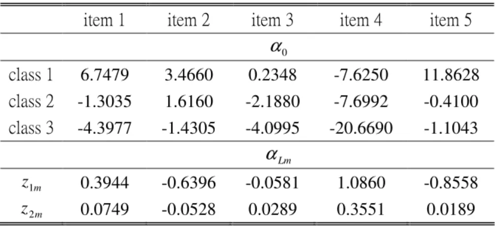
Table 1: Values of

α

₀

and

α

Lm

in 3-class model ...32

Table 2

Table 2

Table 2

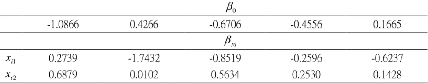
Table 2: Values of

β

₀

and

β in 3-class model ...32

_pj

Table 3:

Table 3:

Table 3:

Table 3: Values of

α and

₀

α

_Lm

in 6-class model ...33

Table 4:

Table 4:

Table 4:

Table 4: Values of

β and

₀

β in 6-class model ...33

pj

Table 5:

Table 5:

Table 5:

Table 5: Values of

α and

₀

α

Lm

in 2-class model ...34

Table 6:

Table 6:

Table 6:

Table 6: Values of

β and

₀

β in 2-class model ...34

_pj

Table 7:

Table 7:

Table 7:

Table 7: Average parameters estimations for 100 replication in 3-class model, N=100 ..35

Table 8:

Table 8:

Table 8:

Table 8: Average parameters estimations for 100 replication in 3-class model, N=100 ..36

Table 9:

Table 9:

Table 9:

Table 9: Average conditional Probability for 100 replication in 3-class model, N=100 ..37

Table 10:

Table 10:

Table 10:

Table 10: Average Latent Prevalences for 100 replication in 3 class model, N=100 ....38

Table 11:

Table 11:

Table 11:

Table 11:

Average Correlation Coefficients for 100 replication in 3-class model, N=100.

...38

Table 12:

Table 12:

Table 12:

Table 12: Average parameters estimations for 100 replication in 3-class model, N=500.

...39

Table 13

Table 13

Table 13

Table 13: Average parameters estimations for 100 replication in 3-class model, N=500.

...40

Table 14

Table 14

Table 14

Table 14:::: Average conditional Probability for 100 replication in 3- class model, N=500.

...41

Table 15:

Table 15:

Table 15:

Table 15: Average Latent Prevalences for 100 replication in 3 class model , N=500 ...42

Table 16:

Table 16:

Table 16:

Table 16: Average Correlation Coefficients for 100 replication in 3-class model, N=500

...42

Table 17:

Table 17:

Table 17:

Table 17: Average parameters estimations for 100 replication in 6-class model, N=300.

Table 18:

Table 18:

Table 18:

Table 18: Average parameters estimations for 100 replication in 6-class model, N=300.

...47

Table 19:

Table 19:

Table 19:

Table 19: Average conditional Probability for 100 replication in 6-class model, N=300.

...48

Table 20:

Table 20:

Table 20:

Table 20: Average Latent Prevalences for 100 replication in 6-class model, N=300 ....52

Table 21:

Table 21:

Table 21:

Table 21: Average Correlation Coefficients for 100 replication in 6-class model, N=300.

...52

Table 22:

Table 22:

Table 22:

Table 22: Average parameters estimations for 100 replication in 6-class model, N=1000.

...53

Table 23:

Table 23:

Table 23:

Table 23: Average parameters estimations for 100 replication in 6-class model, N=1000.

...57

Table 24:

Table 24:

Table 24:

Table 24: Average conditional Probability for 100 replication in 6-class model, N=1000.

...58

Table 25:

Table 25:

Table 25:

Table 25: Average Latent Prevalences for 100 replication in 6-class model, N=1000 ....62

Table 26:

Table 26:

Table 26:

Table 26: Average Correlation Coefficients for 100 replication in 6-class model, N=1000.

...62

Table 27:

Table 27:

Table 27:

Table 27: Average parameters estimations for 100 replication in 2-class model, N=150.

...63

Table 28:

Table 28:

Table 28:

Table 28: Average parameters estimations for 100 replication in 2-class model, N=150.

...64

Table 29:

Table 29:

Table 29:

Table 29: Average conditional Probability for 100 replication in 2-class model, N=150.

...64

Table 30:

Table 30:

Table 30:

Table 30: Average Latent Prevalences for 100 replication in 2-class model, N=150 ...67

Table 31:

Table 31:

Table 31:

Table 31: Average Correlation Coefficients for 100 replication in 2-class model, N=150.

...67

Table 32:

Table 32:

Table 32:

...68

Table 33:

Table 33:

Table 33:

Table 33: Average parameters estimations for 100 replication in 2-class model, N=700.

...70

Table 34:

Table 34:

Table 34:

Table 34: Average conditional Probability for 100 replication in 2-class model, N=700.

...70

Table 35:

Table 35:

Table 35:

Table 35: Average Latent Prevalences for 100 replication in 2-class model, N=700 ...72

Table 36:

Table 36:

Table 36:

Table 36: Average Correlation Coefficients for 100 replication in 2-class model, N=700.

List of Figures

Figure 1: An example of k-means algorithm procedure ...18

Figure 2: An example of hierarchical algorithm procedure ...20

Figure 3

Figure 3

Figure 3

1. Introduction

Latent class analysis (LCA), originally described by Green (1951) and systematically

developed by Lazarsfeld and Henry (1968), Goodman (1974), has been found useful

for classifying objects based on their responses to a set of categorical items. The basic

model postulates an underlying categorical latent variable, say, J categories, and

measured items are assumed independent of one another within any category of the

latent variable. Observed relationships among measured variables are thus assumed to

result from the underlying classification of the data produced by the categorical latent

variable. Latent class analysis may legitimately be viewed as the analog of cluster

analysis. The term cluster analysis (first used by Tryon, 1939) encompasses a number

of different algorithms and methods for grouping objects of similar kind into

respective categories. In this research, instead of grouping objects of “similar kind”

into respective categories, we use hierarchical and k-means ideas of clustering

methods with the correlation among items as the distance measure to group objects

such that, for all objects who belong to the same latent class, items are ”independent”.

Recently several authors extended the LCA model to describe the effects of

measured covariates on the underlying mechanism (Dayton and Macready, 1988; Van

der Heijden, Dessens and Bökenholt, 1996; Bandeen-Roche, Miglioretti, Zeger and

Rathouz, 1997), or on measured item distributions within latent levels (Melton, Liang

and Pulver, 1994). These extended LCA models are called the regression extension of

latent class analysis (RLCA) models. For the RLCA model, by using the

marginalizing techniques to eliminate covariate effects from both the latent variable

and measured indicators (Huang 2005), our clustering idea can be also applied to the

reduced LCA model to estimate the latent class membership. By viewing the latent

2. Literature review

2.1 Latent class analysis (LCA)

Latent class analysis (LCA) aims to classify objects based on their responses to a set

of categorical items. To introduce the methodology, let

Y_{i =}(Y_i1,L,Y_iM)T _{denote a} set of M observable polytomous indicators for the ith individual in a study sample of N persons. Y_im, m=1,…,M can take values {1,L,K_m}_{, where}

_≥

₂

m

K . The basic model postulates an underlying categorical latent variable S_i=1,…,J for individual i; within any category of the latent variable, the measured indicators are assumed to be independent of one another. Therefore, the distribution for Y_i can be expressed as follows:

,

}

)]

|

[Pr(

)

{Pr(

)

,

,

Pr(

1 1 1 1 1

∑

∏∏

= = =

=

=

=

=

=

=

J j M m K k y i im i M iM i m mk

j

S

k

Y

j

S

y

Y

y

Y

L

_(2.1)

where ymk

=

1if y_m

=

k; 0 otherwise. The LCA model assumes that , j) Pr(S , ) | Pr(Yim

=

k Si

=

j

=

pmkj _i

=

=

η

_j (2.2) i=1,…,N; m=1,…,M; k=1,…,K_m; j=1,…,J. Thus, the model treats class membership probabilities,

η

_j, and item response probabilities conditional on class membership,

mkj

p , as homogeneous over individuals. Heuristically,

η

_j is the population prevalence of class j, and p_mkj is the probability of an individual in class j being at level k of Y_im. Goodman (1974) provided an excellent overview of the LCA model, including a maximum likelihood strategy for estimating model parameters, conditions to determine local model identifiability, a strategy to test overall model fit, and the use of constraints to identify models.

Huang and Bandee-Roche (2004) extend the latent class analysis to allow both the probabilities of latent class membership and the distribution of observed responses given latent class membership to be functionally related to concomitant variables, while preserving model identifiability. By allowing covariate effects on latent class probabilities, the model can summarize the effect of risk factors on the underlying mechanism. In the case of incorporating covariates into conditional probabilities, the model can also adjust for characteristics that determine responses other than underlying classes, hence improving the accuracy of classifying individuals. For example, in evaluating functional disability, some data have suggested that women tend to rate tasks as “difficult” more readily than men independently of ability (Bandeen-Roche, Huang, Munoz, & Rubin, 1999). Without adjusting for a gender effect, the model might well classify some men and women with identical underlying functioning differently (men as “able”, women as “disabled”).

Let (x _i , z _i ) be the concomitant covariates of the ith person, where x_i=

[

1

,

x

_i1

,

L

,

x

_ip

]

T _{are primary covariates hypothesized to be associated with latent} class S_i, and z_i=[z_i1,…, z_iM] with z_im=[1, z_im1,…, z_imL]T, m=1,…,M are secondary covariates used to build direct effects on measured indicators. The sets of covariates may include any combination of continuous and discrete measures and two sets of covariates may be mutually exclusive or overlap. The basis RLCA equation can be stated as follows:

∑

_∏∏

= = =













+

=

=

=

J j M m K k mk T im mj y mkj j i i M iM i m mk

_z

p

z

y

Y

y

Y

1 1 1 T i 1 1

,

,

|

x

,

)

(

x

)

(

)

Pr(

L

η

β

γ

α

_(2.3)

with

η

_j (x _i ) and p_mkj(z_im) defined as in the generalized linear framework (McCullagh and Nelder, 1989). Often, (2.3) is implemented by assuming generalized logit link functions (Agresti, 1984):

iP Pj i j j J j

x

x

β

β

β

β

η

β

η

+

+

+

=

















L

1 1 0 T i T i

)

x

(

)

x

(

log

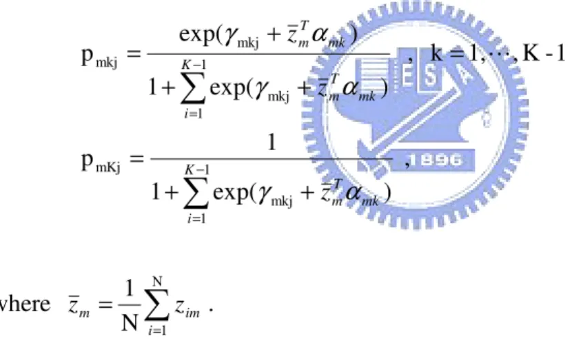
(2.4) and imL Lmk im mk mkj mk T im mj mKj mk T im mj mkj

z

z

z

p

z

p

α

α

γ

α

γ

α

γ

+

+

+

=

















+

+

L

1 1 ' ' '

)

(

)

(

log

J , , 1 j 1); -(J , 1, j ); 1 (K , 1, k M; , 1, m N; , 1, i ' m L L L L L

=

=

− = = = (2.5) Notice that in the conditional probability model (2.5), we allow unrestricted intercepts and level- and item-specific covariate coefficients, but we do not allowing the coefficients to vary across classes (i.e.,

α

_qmk is dependent on m, k but independent of j). This constraint is logical if the primary purpose of modeling conditional probabilities is to prevent possible misclassification by adjusting for characteristics associated with item measurements. It is also necessary to unambiguously distinguish covariate effects on measured response probabilities from covariate effects on class probabilities. Three assumptions complete (2.3):

(C1)

Pr(

Y

_i1

=

y

₁

,

L

,

Y

_iM

=

y

_M

|

S

_i

,

x

_i

,

z

_i

)

=

Pr(

Y

_i1

=

y

₁

,

L

,

Y

_iM

=

y

_M

|

S

_i

,

z

_i

)

;

(C2)

Pr(

S

i

=

j

|

x

i

,

z

i

)

=

Pr(

S

i

=

j

|

x

i

)

;

(C3)

∏

=

=

=

=

=

M m im i m im i i M iM i

y

Y

y

S

z

Y

y

S

z

Y

1 1 1

,

,

|

,

)

Pr(

|

,

)

Pr(

L

_.

Huang and Bandee-Roche (2004) provided an excellent overview of the RLCA model, including model identification, Expectation-Maximization algorithm for parameter estimation, standard error calculation, convergent properties, and

modeling software.

2.3 Marginalization of the regression extension of latent class model

Here we introduce a process to “eliminate” the covariate effects, hence “marginalize” the RLCA model (2.3). The marginalization process (Huang 2005) includes two stages. Stage 1 aims to eliminatez_i. Stage 2 applies the marginalization property used Bandeen-Roche et al. (1997) to average x effects out of the latent prevalence. _i

2.3.1. Marginalizing the covariate effects on conditional probabilities

The key to marginalizing over z_i is that the process must yield random variables that follow a finite mixture distribution that is both independent of z_i and has J mixing components. One strategy for achieving such marginalization can be motivated by the properties of added variable plots for linear regression models.

Consider the linear model

=

x₁T

β

₁

+

x₂T

β

₂

+

ε

Y , (2.6) where

ε

has mean 0 and variance matrix V. Let Y~ denote the residuals of regressing Y on

x

₂, and W = V−1 be the weight matrix. Then, it is well known that if

1

x

and

x

₂ are orthogonal (i.e., x₁ xT₂ =0

W ), Y~ has mean x₁T

β

₁

and variance V. Hence, the simple linear regression of Y~ on

x

₁ yields exactly the same inferences about

β

₁ as if we performed the analysis on the more complicated model (2.6) (Cook and Weisberg, 1982). Viewing the just-described stability of

β

1 as analogous

to the desired stability of latent class dimension, J, the added variable property can be applied to model (2.5) to obtain marginalized conditional probabilities.

To present the key ideas more clearly, henceforth, the measured indicators )

Y , , Y

( _i1 L _{iM are assumed to be binary (i.e.,}

_K

_K

₂

M

1

= L

=

=

). To make the analogy

adjusting for z_im, separately for each m. To see this, let Sij =I(S_i = j)=1

if

S

i

=

j

;

0 otherwise, for i = 1,…, N; j = 1,…, J-1. we can reparameterize (2.5) as log [ ( | , )]_{= +}( ) for i₌1,L,N; m₌1,L,M., m T c im m T i c im i im S Z S Z Y E it

γ

α

(2.7) where

S

i

=

[

1

,

S

i1

,

L

,

S

i(J−1)

]

T; T mL imL m im z z z z ), ,( )] [(

Z_imc = ₁− ₁ L − _{, (“centered” covariate vector)} (1/N) z N 1 i imp

∑

= = mp z ;

.

]

,

,

[

and

;

]

,

,

,

[

_{m0 m1 m(J 1)} T _{m 1m Lm} T m

γ

γ

γ

α

α

α

γ

₌

L

₌

L

−

Therefore, for any realization of S_i, (2.7) is a logistic regression with dependent variable:Y_imp and predictors:S_i, Z . c_im

Next, the problem becomes how to calculate residuals from the generalized linear model M , 1, m N; , 1, i for ) ( )] | ( [ log ₌ * ₌ L ₌ L m T c im c im im Z Z Y E it

α

. (2.8)

The “pseudo-residuals” are given by

]

ˆ

Y

[

)

V

ˆ

(

]

R

,

,

R

[

R

_m

=

_1m

_L

_Nm T

=

_m −1 _m

−

u

_m , (2.9) where “hat” represents the estimated values;

) V , , V ( diag V_{m = 1m} L _{Nm , V Var(Y )} im im = ; T Nm m m [Y , ,Y ] Y _{= 1} L _{; E(Y |Z}c₎ m m m u = .

If

x

_i and

z

_im are independent, we can extract the Zc_im from conditional probabilities by treating the residuals from the model (2.8) as new response variables and regressing them on S_i. We substitute the estimate of

γ

_m* in the linear model

M , 1, m N; , 1, i , S R_{im =} T_i * _{+ =} L ₌ L im m

ε

γ

(2.10)

m

γ

can be very close under reasonable regularities. The above results can be extended to the cases where (Y_i1,L,Y_iM)_{are polytomous as in (2.1) and (2.3).}

2.3.2. Marginalizing the covariate effects on latent prevalences

The marginalization of model (2.3) over z_i possesses the nice property that the covariates associated with latent class prevalences,x , can be ignored. _i

2.4 Hierarchical clustering methods

Hierarchical clustering techniques proceed by either a series of successive mergers or a series of successive divisions. Agglomerative hierarchical methods start with the individual objects. Thus, there are initially as many clusters as objects. The most similar objects are first grouped, and these initial groups are merged according to their similarities. Eventually, as the similarity decreases, all subgroups are fused into a single cluster.

Divisive hierarchical methods work in the opposite direction. An initial single group of objects is divided into two subgroups such that the objects in one subgroup are “far from” the objects in the other. These subgroups are then further divided into dissimilar subgroups; the process continues until there are as many subgroups as objects – that is, until each object forms a group.

The results of both agglomerative and divisive methods may be displayed in the form of a two-dimensional diagram known as a dendrogram. As we shall see, the dendrogram illustrates the mergers or divisions that have been made at successive levels.

In this research, we concentrate on agglomerative hierarchical procedures. The following are the steps in the agglomerative hierarchical clustering algorithm for grouping N objects (items or variables):

matrix of distances (or similarities)

D

=

{

d

ik

}

.

2. Search the distance matrix for the nearest (most similar) pair of clusters. Let the distance between “most similar” clusters U and V be

d

_UV .

3. Merge clusters U and V. Label the newly formed cluster (UV). Update the entries in the distance matrix by (a) deleting the rows and columns corresponding to cluster U and V and (b) adding a row and column giving the distances between cluster (UV) and the remaining clusters.

4. Repeat Steps 2 and 3 a total of N-1 times. All objects will be in a single cluster after the algorithm terminates. Record the identity of clusters that are merged and the levels (distances or similarities) at which the mergers take place.

2.5 Ward’s hierarchical clustering method

Ward (1963) considered hierarchical clustering procedures based on minimizing the ‘loss of information’ from joining two groups. This method is usually implemented with loss of information taken to be an increase in an error sum of squares criterion, ESS. First, for a given cluster k, let ESS_kbe the sum of the squared deviation of every item in the cluster from the cluster mean (centroid). If there are currently K clusters, define ESS as the sum of the

ESS

Kor

ESS

=

ESS

1

+

ESS

2

+

L

+

ESS

K. At each step in the analysis, the union of every possible pair of clusters is considered, and the two clusters whose combination results in the smallest increase in ESS (minimum loss of information) are joined. Initially, each cluster consists of single item, and, if there are N items,

ESS

K=0, k=1,2,…,N, so ESS=0. At the other extreme, when all the clusters are combined in a single group of N items, the value of ESS is given by

)

x

x

(

)

x

x

(

1

−

′

−

=

∑

= j N J j

ESS

,

where x is the multivariate measurement associated with the jth item and x is the _j mean of all the items.

The results of Ward’s method can be displayed as a dendrogram. The vertical axis gives the values of ESS at which the mergers occur.

Ward’s method is based on the notion that the clusters of multivariate observations are expected to be roughly elliptically shaped. It is a hierarchical precursor to nonhierarchical clustering methods that optimized some criterion for dividing data into a given number of elliptical groups.

2.6 K-means method

The K-means method is one of the more popular nonhierarchical procedures. MacQueen (1967) suggests the term K-means for describing an algorithm of his that assigns each object to the cluster having the nearest centroid (mean). In its simplest version, the process is composed of these three steps:

1. Partition the objects into K initial clusters.

2. Proceed through the list of objects, assigning an object to the cluster whose centroid (mean) is nearest. (Distance is usually computed using Euclidean distance with either standardized or unstandardized observations.) Recalculate the centroid for the cluster receiving the new object and for the cluster losing the object.

Rather than start with a partition of all objects into K preliminary groups in Step 1, we could specify K initial centroids (seed points) and then proceed to step 2.

The final assignment of objects to clusters will be, to some extent, dependent upon the initial partition or the initial selection of seed points. Experience suggests that most major changes in assignment occur with the first reallocation step.

3. Models

3.1 LCA

Let (Y_i1,L,Y_iM) _{denote a set of M observable polytomous outcome indicators and} i

S denote the unobservable class membership, for the ith individual in a study sample of N persons. Y_im can take values{1,L,K_m}_{, where ≥2}

m

K , m=1,…,M,

and S_i can take values {1,L,J}_{. The latent class analysis model is based on the} concept of conditional independence in the sense that the observed variables are assumed to be statistically independent within latent classes. Therefore, the distribution for (Y_i1,L,Y_iM) _{can be expressed as the finite mixture density:}

∑ ∏∏

= = =

=

=

=

J j M m K k y mkj j M iM i m mk

p

y

Y

y

Y

1 1 1 1 1

,

,

)

{

}

Pr(

L

η

_,

_(3.1)

where

η

j =Pr(Si = j) are the “latent class probabilities” of each underlying variable category, pmkj =Pr(Yim =k|Si = j) are the “conditional probabilities” of the measured responses given the underlying variable category and ymk =I(ym =k) .

For more detail on identifiability, parameter estimations and the test overall model fit, readers may reference Goodman (1974)

3.2 RLCA

To incorporate covariate effects into LCA, let (x_i, z_i) be the associated covariate vector for the ith person, where x_i=

[

1

,

x

_i1

,

L

,

x

_ip

]

T _{are predictors associated with} latent class S_i, and z_i=[z_i1,…, z_iM]; z_im=[1, z_im1,…, z_imL]T with m=1,…M are covariates used to build direct effects on measured indicators. The sets of covariates may include any combination of continuous and discrete measures. To marginalize

the RLCA model (3.2) , we begin by assuming that the two sets of covariates are mutually independent. The basis RLCA equation can be stated as

∑

∏∏

= = =













+

=

=

=

J j M m K k mk T im mj y mkj j i i M iM i m mk

_z

p

z

y

Y

y

Y

1 1 1 T i 1 1

,

,

|

x

,

)

(

x

)

(

)

Pr(

L

η

β

γ

α

_(3.2) with

η

j

(

x

T_i

β

)

and

(

mk

)

T im mj mkj

z

p

γ

+

α

defined as in the generalized linear framework (McCullagh and Nelder, 1989). Often, (3.2) is implemented by assuming generalized logit (Agresti, 1984) link functions:

iP Pj i j j J j

x

x

β

β

β

β

η

β

η

+

+

+

=

















L

1 1 0 T i T i

)

x

(

)

x

(

log

(3.3) and imL Lmk im mk mkj mk T im mj mKj mk T im mj mkj

z

z

z

p

z

p

α

α

γ

α

γ

α

γ

+

+

+

=

















+

+

L

1 1 ' ' '

)

(

)

(

log

J , , 1 j 1); -(J , 1, j ); 1 (K , 1, k M; , 1, m N; , 1, i ' m L L L L L = = − = = = (3.4)

If the regression coefficients in (3.3) or (3.4) are set as 0, model (3.2) reduces to models studied by Melton, Liang and Pulver (1994), Dayton and Macready (1998) or an ordinary latent class analysis (3.1).

Notice that in the conditional probability model (3.4), we allow unrestricted intercepts and level- and item-specific covariate coefficients, but we do not allowing the coefficients to vary across classes (i.e.,

α

_qmk is dependent on m, k but independent of j). This constraint is logical if the primary purpose of modeling conditional probabilities is to prevent possible misclassification by adjusting for characteristics associated with item measurements. Three assumptions complete (3.2):

(C1)

Pr(

Y

_i1

=

y

₁

,

L

,

Y

_iM

=

y

_M

|

S

_i

,

x

_i

,

z

_i

)

=

Pr(

Y

_i1

=

y

₁

,

L

,

Y

_iM

=

y

_M

|

S

_i

,

z

_i

)

;

(C2)

Pr(

S

i

=

j

|

x

i

,

z

i

)

=

Pr(

S

i

=

j

|

x

i

)

;

(C3)

∏

=

=

=

=

=

M m im i m im i i M iM i

y

Y

y

S

z

Y

y

S

z

Y

1 1 1

,

,

|

,

)

Pr(

|

,

)

Pr(

L

_.

For more detail on model assumptions, identifiability and parameter estimations, readers may reference Huang and Bandeen-Roche (2004).

4. Parameter estimations by clustering analysis

The parameters in (3.2) are typically estimated by maximum likelihood (ML) for a fixed number of classes, J. Viewing the class membership S_i as unobservable, the LCA model (3.1) and RLCA model (3.2) becomes a typical incomplete-data problem. Goodman (1974) provided an excellent maximum likelihood strategy for estimating model parameters in (3.1), and Hung and Bandeen-Roche (2004) had successfully used the Expectation-Maximization (EM) algorithm (Dempster, Laird, & Rubin, 1997) to computing ML estimates of the parameters in (3.2) and created a powerful computer module to implement the proposed latent class model (3.2). However implementing the EM algorithm to estimate parameters in finite-mixture models is typically time-consuming. Therefore we propose an alternative clustering analysis strategy to predict parameters in (3.1) and (3.2).

4.1 Latent class membership estimations for LCA

Latent class analysis aims to classify objects based on their responses to a set of categorical items. The basic model postulates an underlying categorical latent variable

i

S =1,…,J for individual i; within any category of the latent variable, the measured indicators are assumed to be independent of one another. Therefore if we can estimate the unobservable class membershipS_i based on model assumption, then it is easy to predict the parameters in (3.1) by viewing the estimated class membership as known variable. We propose the following strategy to estimateS_i.

Here we apply the concept of k-means (MacQueen, 1967) and agglomerative hierarchical methods to group the objects. Notice that rather than grouping the objects into J subgroups such that the objects in one subgroup are “far from” the objects in the other, we try to group objects such that observed variables are statistically

independent within latent classes. Therefore we use sample correlation or sample covariance as the distance in k-means and agglomerative hierarchical methods, and the concept of the ’ loss information’ and ‘minimum loss of information’ in ward’s hierarchical clustering method is included.

First, we introduce how to calculate the sample correlation and sample covariance matrix used in the k-means and agglomerative hierarchical clustering algorithms. For individual i, we transform the M observable polytomous outcome indicators (Y_i1,L,Y_iM)_{to the following dummy variables:}

)

Y

,

,

Y

,

,

Y

,

,

Y

,

Y

,

,

Y

(

Y

~

_{i i11 1( 1) i21 2( 1) iM1 ( 1)}

2 1− − −

=

M K iM K i K i

L

L

L

L

L

with

Y

_imk

₌

I(Y

_im

₌

_k

)

,

m

₌

1,

L

,

M;

k

₌

1,

L

K

_m-1. Then,

[

]

, B B B B B B B B B ) Cov(Y ) Y~ Cov( MM M2 M1 2M 22 21 1M 12 11 imk, i             = = L M O M M L L iqs Y (4.1)

where for the mth item and qth item, B_mq is the block of (K_m −1)×(K_q −1) covariance matrix. Various elements of the variance-covariance matrix of measured indicators are:      ≠ = = − = = ≠ = = = − = = = = − = = q m if ) 1 Y Pr( ) 1 Y Pr( ) 1 Y , 1 Y Pr( (4.2) s k and q m if ) 1 Y Pr( ) 1 Y Pr( s k and q m if ) 1 Y Pr( ) 1 Y Pr( ) 1 Y Pr( ) , Cov(Y iqs imk iqs imk iqs imk iqs imk imk imk Yiqs

These variances were estimated by replacing the probabilities with the sample averages. From sample covariance matrix, we can also calculate the sample

correlation matrix as 2 1 -i 2 1 -D~ ) Y~ Cov(

D~ , where D~ ₌diag(Bˆ₁₁,Bˆ₂₂,L,Bˆ_MM) _{. The} following are the steps in the k-means and agglomerative hierarchical clustering

algorithm separately.

The K-means algorithm:

1. Partition the objects into K initial clusters.

2. Proceed through the list of objects, assigning an object to the cluster which reaching ‘minimum loss of independence’.

3. Repeat Step2 until no more reassignments take place.

In Step 1, we first specify K initial centroids (seed points) and then proceed through the list of objects, assigning an object to the cluster whose centroid (mean) is nearest. (Distance is computed using Euclidean distance.) To reach enough sample size such that the sample covariance/correlation is meaningful, it is necessary to adjust the number of objects in each initial cluster. Therefore, once existing an one initial cluster including members less than we expect, we repartition the objects “randomly” and “evenly” into K initial clusters.

Next, we shall introduce what the minimum loss of independence is in Step2. For a given cluster k, let

MCov

_k be the mean of the absolute values of entries in non diagonal blocks of sample correlation matrix (or sample covariance matrix) for the M observable polytomous outcome indicators. For a given object, if it is assigned to some cluster j, we define the loss of independence LoI as the sum of the _j

MCov

_k

or (j)K

(j) 2 (j)

1

j

MCov

MCov

MCov

LoI

=

+

+

L

+

_{, where} (j)

k

MCov is the mean of the absolute values of non-diagonal-block entries of Cov(Y~i) after the object being assigned to cluster j . For a given object, after assigning through K clusters, we can get LoI , j= 1,…, K. The smaller the value of _j LoI is, the more independent the _j

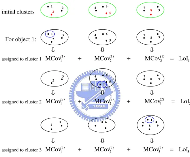
Figure 1: An example of k-means algorithm procedure. Step1: Partition the 9 objects into 3 initial clusters. Step2: What cluster will the object 1 be assigned to?

Assigning the object 1 to the cluster 1,2 and 3 separately, we can get LoI1,

LoI₂ and LoI₃. Assign the object 1 to the cluster which reaching “minimum loss of independence”.

Proceed through the objects 2-9, repeat above procedure. Step3: Repeat Step2 until no more reassignments take place.

observed variables for objects within cluster j are. So, we take the minimum LoI as _j the ‘minimum loss of independence’ and assign a given object to the cluster corresponding to the minimum loss of independence. An example of k-means algorithm procedure can be found in Figure1.

The agglomerative hierarchical clustering algorithm:

initial clusters

2 1 _{3 4} 5 8 6 ₇ 9 2 1 _{3 4} 5 8 6 ₇ 2 1 3 4 5 8 6 ₇ 9 2 3 6 7 _{8 9} 1 2 (2) 3 (2) 2 (2)

1

MCov

MCov

LoI

MCov

+

+

=

1 (1) 3 (1) 2 (1)

1

MCov

MCov

LoI

MCov

+

+

=

3 (3) 3 (3) 2 (3)

1

MCov

MCov

LoI

MCov

+

+

=

For object 1:

assigned to cluster 1 assigned to cluster 2 assigned to cluster 3 9

1. Start with N clusters, each cluster consists of a single object.

2. If there are some objects whose M items are all the same, then we merge them together. Otherwise, skip this step.

3. The union of every possible pair of clusters is considered, and the two clusters U and V whose combination results in the minimum loss of independence are merged. Label the newly formed cluster (UV).

4. Repeat Step 3 until all objects will be in a single cluster after the algorithm terminates. Record the identity of clusters that are merged and the levels (minimum loss of independence) at which the mergers take place.

Now we will introduce the minimum loss of independence in Step3 in the agglomerative hierarchical clustering algorithm. For currently K clusters, if a cluster U is merged to the other cluster V, then the K clusters decrease to K-1 clusters. We defined the loss of independence for cluster U being merged to cluster V, LoI_{(V, U)}, as the sum of

MCov

k(defined in the K-means algorithm) of each cluster:

U) (V, K U) (V, 1 U U) (V, 1 -U U) (V, 1 U)

(V,

MCov

MCov

MCov

MCov

LoI

=

+

L

+

+

+

+

L

+

.

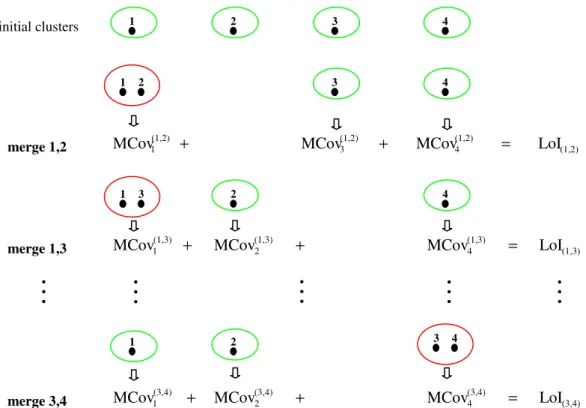
For currently K clusters, we can get C K₂ LoI_{(V, U)}, where (V, U) belong to the union of every possible pair of clusters. The smaller the value of LoI_{(V, U)} is, the more independent the observed variables for objects within the newly formed cluster (UV) are. So, we take the minimum LoI_{(V, U)} as the ‘minimum loss of independence’ and merge the two clusters U and V whose combination results in the minimum loss of independence. An example of hierarchical algorithm procedure can be found in Figure2.

The results of agglomerative hierarchical clustering method can be displayed as a dendrogram. The vertical axis gives the values of minimum loss of independence at which the mergers occur.

4.2 Latent class membership estimations for RLCA

The k-means and agglomerative hierarchical clustering algorithms are based on the model (3.1) where no covariates are incorporated. The two algorithms also work for

initial clusters 1 (1,2) (1,2) 4 (1,2) 3 (1,2)

1 MCov MCov LoI

MCov + + = merge 1,2 2 3 4 1 2 3 4 (1,3) (1,3) 4 (1,3) 2 (1,3)

1 MCov MCov LoI

MCov + + = merge 1,3 1 3 4 (3,4) (3,4) 4 (3,4) 2 (3,4)

1 MCov MCov LoI

MCov + + = merge 3,4 3 4 2 2 1

M

M

M

M

M

Figure 2: An example of hierarchical algorithm procedure.

Step1: Star with 4 initial clusters, each cluster consists of a single object. Step2: Which pair of clusters will be merged?

Consider the union of 6 (=C24) possible pair of clusters, we can get

LoI(1,2), LoI(1,3), LoI(1,4), LoI(2,3), LoI(2,4)and LoI(3,4). Merge the pair of

clusters whose combination results in the “minimum loss of independence”.

the model (3.2) under eliminating the covariate effects (Huang2005), hence “marginalize” the model (3.2).

The key to marginalizing over zi is that the process must yield random variables that follow a finite mixture distribution that is both independent of z_i and has J mixing components. One strategy for achieving such marginalization can be motivated by the properties of added variable plots for linear regression models. The conditional probabilities (3.4) can be viewed as fitting a logistic regression of Yim on

i

S adjusting for z_im, separately for each m. Next the problem becomes how to calculate residuals from the generalized linear model:

log [ ( | )]₌( ) * for i₌1,L,N; m₌1,L,M. m T c im c im p im Z Z Y E it

α

(4.3) where

“p” denotes polytomous responses;

Y

_imp

[

Y

_im1

,

,

Y

_{im(K 1)}

]

T m−

=

L

_and

_Y

_I(Y

₎

im imk

=

=

k

; T mL imL m im z z z z ), ,( )] [(

Z_imc = ₁− ₁ L − _{(“centered” covariate vector), (1/N) z}

N 1 i imp

∑

= = mp z ;

Under polytomous item responses, the pseudo-residual of ith participant’s mth response item is

Y

imp p im

ˆ

)

(

)

V

ˆ

(

R

imp 1 p im

=

−

µ

− , (4.4) where “hat” denotes the estimated values;

R

p_im

[

R

_im1

,

,

R

_{im(K )}

]

T

m

L

=

;V Var(Yp ) 1m p im = ; ) Z | E(Y_mp c_m p m =

µ

; and

i

₌

1,

L

,

N;

m

₌

1,

L

,

M,

k

₌

1,

L

,

K

_m

.

_{With the nice} property that the covariates associated with class prevalencesx can be ignored and i under the assumption of

x

i and

z

imare independent, we can treating the residuals

from the model (4.1) as new response variables. Details of the above the marginalization process can be found in Huang (2005) and in section 2.3 of this thesis. We can classify objects based on the new response variables R_imp to a set of

agglomerative hierarchical clustering algorithms in section 4.1, besides the estimation of the covariance matrix Cov(Y~i) in (4.1), evaluated as 

   − R ~ ) 11 n 1 -I ( R~ 1 n 1 ' n T _,

where R~ is the residual matrix of n objects.

4.3

Parameter estimation by viewing estimated latent class as

known variable

Denote the estimated latent class as

Sˆ

_i for individual i. We transform (3.3) and (3.4) as the following form:

iP Pj i j

x

β

x

β

β

+

+

+

=

















=

=

L

1 1 0 i i i i

)

x

|

J

Sˆ

Pr(

)

x

|

j

Sˆ

Pr(

log

(4.5) and imL Lmk im mk J i J mk i mk mk i im i im

z

z

S

S

S

K

Y

S

k

Y

α

α

γ

γ

γ

+

+

+

+

+

+

=

















=

=

− −

L

L

1 1 ) 1 ( * ) 1 ( 1 * 1 * 0 i i

ˆ

ˆ

)

z

,

ˆ

|

Pr(

)

z

,

ˆ

|

Pr(

log

(4.6) 1) -(J , 1, j ); 1 (K , 1, k M; , 1, m N; , 1, i m L L L L = − = = =

where Sˆij =I(Sˆi = j)

.

Notice that

γ

mk

=

γ

mkJ

γ

mkj

=

γ

mkj

−

γ

mkJ

* 0 *

and

in (3.4).

Then, we can easily predict the parameters in (3.2) by multinomial logistic regression (4.5) and (4.6).

5. Simulation study

The simulation study aims to examine the performance of the proposed approach.

5.1 Generated data from the RLCA model

Here, three different RLCA (3.2) models were simulated. One was a three-class RLCA with five two-level measured indicators, two covariates associated with conditional probabilities, and two covariates associated with latent prevalences (i.e., J=3, M=5, K1 = L=K5 =2, P=L=2). Another was a six-class RLCA with five three-level measured three-level measured indicators, two covariates associated with conditional probabilities, and two covariates associated with latent prevalences (i.e., J=6, M=5, K₁ = L=K₅ =3, P=L=2). The other was a two-class RLCA with the same indicators and covariate setting as the six-class model (i.e., J=2, M=5,

3 K

K₁ = L= ₅ = , P=L=2). For each model, the model parameters 1} -J , 1, j , { ₌ L pj

β

for each _p∈{0,1,L,P}_{, { ,j=1,}L_,J} jmk

γ

for all m,k, and 1)} -(K , 1, k M; , 1, m , { ₌ L ₌ L _m qmk

α

for all q, were given. Table 1~6 shows the

values of the model parameters for the three model separately. We got the covariates of 3-class model from the subjects who joined the Multidimensional Psychopathological Study on Schizophrenia (MPSS) or the Study on Etiological Factors of Schizophrenia (SEFOS). We got the covariates of 6-class model and 2-class model from the subjects who joined the Multidimensional Psychopathology Group Research Projects (MPGRP), MPSS or SEFOS. In each model, the covariates associated with conditional probabilities include variables of sex and age (year), and the covariates associated with latent prevalences include variables of occupation (with versus without occupation) and dprime, which is the sensitivity index of the

We fit each model under several different sample sizes. For the three-class RLCAs, the selected sample sizes were 100 and 500, which gave roughly 3 and 16 individuals per parameter of RLCA (3.2), respectively. For the six-class RLCAs, the selected sample sizes were 300 and 1000, which gave roughly 3 and 10 individuals per parameter, respectively. For the two-class RLCAs, the selected sample sizes were 150 and 700, which gave roughly 3 and 16 individuals per parameter, respectively. The observable measurements

Y

_i were then generated from each different model structure with 100 replications.

5.2 Simulation results

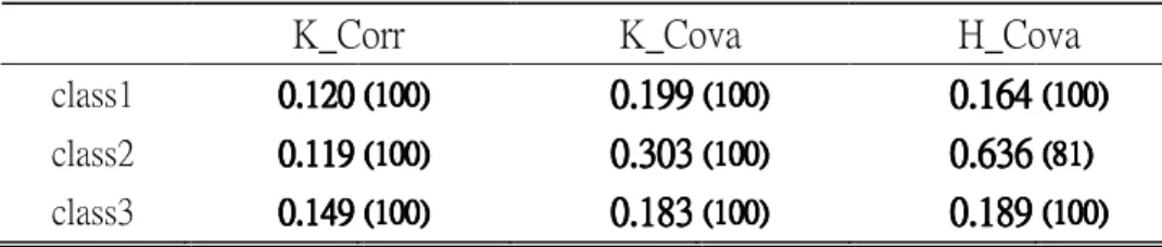
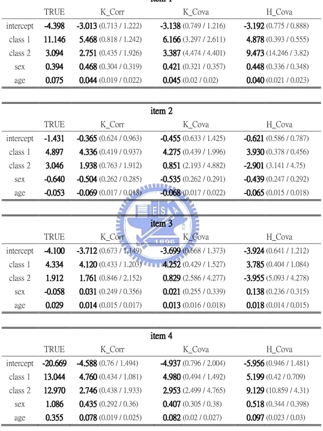
In each case, the results of simulation study are represented in five tables which include the average parameters estimates (listed in two tables), average conditional probabilities, average latent prevalences and average correlation coefficients for 100 replications, separately. We shall explain these results later. The simulation results for 3-class model with 100 sample sizes are presented from Table 7 to Table 11. The simulation results for 3-class model with 500 sample sizes are presented from Table 12 to Table 16. The simulation results for 6-class model with 300 sample sizes are presented from Table 17 to Table 21. The simulation results for 6-class model with 1000 sample sizes are presented from Table 22 to Table 26. The simulation results for 2-class model with 150 sample sizes are presented from Table 27 to Table 31. The simulation results for 3-class model with 750 sample sizes are presented from Table 32 to Table 36. According to Table 7 ~ Table 36, we can see that these results of the k-means method using correlation coefficients measurement are similar to those of k-means method using covariance measurement. So, we shall discard the results of k-means method using covariance measurement in the following discussion.

Table 16 of 3-class model with 500 sample sizes.

Average parameters estimations:

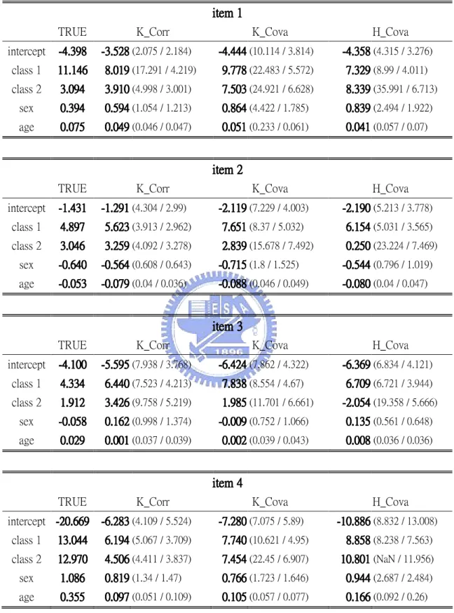
Table 12 and Table 13 under the column “TRUE” include all

{

β

_pj,

γ

_jmk,

α

_qmk

}

in simulated data. All average of

{

β

_pj,

γ

_jmk,

α

_qmk

}

estimates got from the k-means method using correlation coefficients measurement (K_Corr) and covariance measurement (K_Cova) separately and the hierarchical method using covariance measurement (H_Cova) are also shown in Table 12 and Table 13. Why not correlation coefficients measurement for Hierarchical method? At the initial stage, correlation coefficients in two objects are always one. Table 12 and Table 13 can demonstrate that the parameters estimates got from the k-means method are not bad compared to the true parameters. But the parameters estimates got from the hierarchical procedure are poor. The bad performance of the hierarchical procedure is result from there is no provision for a reallocation of objects that may have been “incorrectly” grouped at an early stage. Furthermore, the hierarchical procedure is sensitive to cluster structure. This means that hierarchical procedure have the chance to perform more well only when there is clear cluster structure than when there is no clear cluster structure.

Table 12 and Table 13 also include the standard errors of parameters estimates in doing multinomial regressions, (4.1) and (4.2), and the average sample standard errors of the parameters estimates for 100 replications. The sample standard errors of the estimates for 100 replications include the variation of doing multinomial regression and creating cluster membership. Because we use the multinomial regression to estimate parameters under the assumption of known cluster membership, the standard errors of parameters estimates in doing multinomial regression did not include the variations of creating cluster membership. Therefore, the standard errors of parameters estimates in doing multinomial regressions should be smaller than the

sample standard errors of the estimates for 100 replications. This is demonstrated in Table 12 and Table 13. However this is not demonstrated in Table 7 and Table 8 for the 3-class model with 100 sample sizes which gave very few individuals per parameter. For the sparse data, the estimated standard errors of parameters estimates in doing multinomial regressions are not accurate. Therefore, the standard errors of parameters estimates in doing multinomial regressions are not always smaller than the sample standard errors of the estimates over 100 replications for the 3-class model with 100 sample sizes.

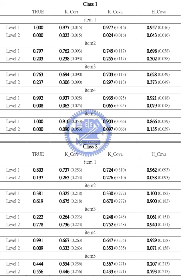
Average conditional probabilities:

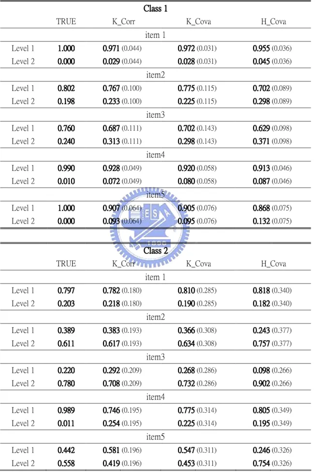
Table 14 under the column “TRUE” displays the RLCA conditional probabilities evaluated at the sample means of the incorporated covariates:

,

)

exp(

1

1

p

1

-K

,

1,

k

,

)

exp(

1

)

exp(

p

1 1 mkj mKj 1 1 mkj mkj mkj

∑

∑

− = − =

+

+

=

=

+

+

+

=

K i mk T m K i mk T m mk T m

z

z

z

α

γ

α

γ

α

γ

L

where

∑

= = N 1 N 1 i im m z z .

The average of estimated conditional probabilities over 100 replications with k-means (K_Corr and K_Cova) and hierarchical (H_Cova) methods are also shown in Table 14. The estimated conditional probabilities for k-means and hierarchical methods are: j clsss in s individual of number the Y of k level at being j clsss in s individual of number the im pˆ_mkj =

Overall, the average conditional probabilities for the k-means method are more closed to the true conditional probabilities than the average conditional probabilities for the hierarchical method.