This article was downloaded by: [National Chiao Tung University 國立交通大學] On: 28 April 2014, At: 05:29
Publisher: Taylor & Francis
Informa Ltd Registered in England and Wales Registered Number: 1072954 Registered office: Mortimer House, 37-41 Mortimer Street, London W1T 3JH, UK
Production Planning & Control: The
Management of Operations
Publication details, including instructions for authors and subscription information:
http://www.tandfonline.com/loi/tppc20
A multiple criteria decision-making model for
justifying the acceptance of rush orders
M. C. Wu & S. Y. Chen
Published online: 15 Nov 2010.
To cite this article: M. C. Wu & S. Y. Chen (1997) A multiple criteria decision-making model for justifying the acceptance of rush orders, Production Planning & Control: The Management of Operations, 8:8, 753-761, DOI: 10.1080/095372897234641
To link to this article: http://dx.doi.org/10.1080/095372897234641
PLEASE SCROLL DOWN FOR ARTICLE
Taylor & Francis makes every effort to ensure the accuracy of all the information (the “Content”) contained in the publications on our platform. However, Taylor & Francis, our agents, and our licensors make no representations or warranties whatsoever as to the accuracy, completeness, or suitability for any purpose of the Content. Any opinions and views expressed in this publication are the opinions and views of the authors, and are not the views of or endorsed by Taylor & Francis. The accuracy of the Content should not be relied upon and should be independently verified with primary sources of information. Taylor and Francis shall not be liable for any losses, actions, claims, proceedings, demands, costs, expenses, damages, and other liabilities whatsoever or howsoever caused arising directly or indirectly in connection with, in relation to or arising out of the use of the Content.
This article may be used for research, teaching, and private study purposes. Any substantial or systematic reproduction, redistribution, reselling, loan, sub-licensing, systematic supply, or distribution in any form to anyone is expressly forbidden. Terms & Conditions of access and use can be found at http://www.tandfonline.com/page/terms-and-conditions
A multiple criteria decision-making model for
justifying the acceptance of rush orders
M. C. WU and S. Y. CHEN
Keywords rush order, multiple objective programming, e-constraints
A bstract. Rush orders are immediate customer demands that
exceed the expectation of a currently eective MPS ( master
production schedule) . Decision-makers are often hesitant in the decision of accepting such orders. This paper presents a multiple criteria decision-making model for justifying the acceptance of rush orders for an assembly-to-order production system. Four criteria or production objectives are simultane-ously considered and a multiple objective programming tech-nique, the e-constraints approach, is adopted to solve the decision-making problem. This model could give the cost esti-mation for producing a rush order under various combinations of production objectives. The computed cost value could serve as a valuable reference for justifying the economics of accepting the rush order, and help to determine its pricing strategy.
1. Introduction
This paper investigates the decision-making problem presented by rush orders. Rush orders are immediate
customer demands that cannot be eectively supplied by performing the current master production schedule ( MPS) . In a dynamic market, rush orders are frequently faced by manufacturing companies, especially by those doing OEM business ( making products for other Firms’ brands) in developing countries. The decision for accep-ting or rejecaccep-ting a rush order often puzzles decision-makers. Marketing department tends to accept it for increasing sales and the number of future customers: con-versely, the production department tends to reject it to avoid the frequent change of MPS and the increase of production cost. To resolve the trade-o issue, an analy-tic model for justifying the acceptance of rush orders is required.
Since rush orders are immediate demands, if they are accepted, their production time should be scheduled in the ® rst few periods of the new MPS. However, such a decision is forbidden in a `freezing scheduling’ environ-ment. The concept of `freezing scheduling’ advocates that
A uthors: M. C. Wu and S. Y. Chen, Department of Industrial Engineering and Management, National Chiao Tung University, Hsin Chu, Taiwan
M. C. Wu is currently a professor at the Department of Industrial Engineering and
Management, National Chiao Tung University, Taiwan. He received a BS degree in electronic engineering from National Chiao Tung University in 1977, the MBA degree from Chen Chi University ( Taiwan) in 1979, and MS and PhD degrees in industrial engineering from Purdue University in 1984 and 1988, respectively. His research interests include production management and CAD/CAM.
S. Y. Ch e ncurrently serves in the army. He received BS and MS degrees in industrial
engineer-ing and management from National Chiao Tung University. This research is a part of his MS thesis work.
0953-7287/97 $12´00 Ñ 1997 Taylor & Francis Ltd.
the MPS should be replanned periodically to respond to the updated demand data, while the ® rst few periods of the MPS should be frozen in each planning cycle to accommodate the committed production resources. This concept is widely adopted in industry and much relevant literature has been published ( Chung and Krajewski 1986, Lin and Krajewski 1992, Sridharan and Berry 1990) . Such studies unquestionably would suggest the rejection of rush orders.
An alternative attempt to justify the acceptance of rush orders is by applying previous studies in aggregate pro-duction planning ( APP) to replan the MPS and compute the increased production cost. However, at the concerned decision point, some production resources or purchasing activities associated with the original MPS have been committed. And the cost of such commitments has sel-dom been discussed in previous APP studies ( Deckro and Herbert 1984, Masud and Hwang 1980, Nam and Logendran 1992, Rakes et al. 1984, Vercellis 1991) . Therefore, the decision-making problem presented by rush orders cannot be directly solved by existing APP approaches.
This paper proposes a multiple objective programming model for justifying the acceptance of rush orders, in which the cost caused by commitments of the original MPS has been considered. Four production objectives for the decision-making are concerned, which involve ( 1) minimizing the extra spending for producing the rush order, ( 2) minimizing the shipping delay of crucial orders, ( 3) minimizing the demand of cash or quick assets, and ( 4) minimizing the inventory level. Of the existing multiple objective programming techniques ( Steuer 1986) , this research adopts the e-constraints approach. That is, one of the four objectives is considered as the main objective which is to be minimized if possible and the other three are taken as constraints by giving their upper bounds.
The proposed model can be used to compute the cost for producing a rush order under various combinations of production objectives. This cost value would provide good reference for justifying the acceptance of the rush order and help determine its pricing strategy. Moreover, the new MPS suggested by the model is optimal in the criteria of the main objective.
2. A ssumptions of production systems
The production system concerned in this research is an assembly-to-order factory where products are assembled from various types of components upon request of custo-mer orders ( Krajewski and Ritzman 1987) . Also, the system is assumed to be a single-stage system; that is, all the components or materials are purchased from
out-side vendors. Some other assumptions concerning the product structures as well as relevant production planning activities are given below.
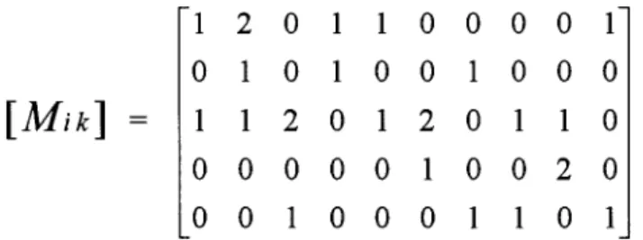
( 1) P roduct structures: multiple products are produced and they share the use of some common materials. The usage of common materials can be described by a product± material relationship ( PMR) matrix as shown in Figure 1. The PMR matrix consists of
n rows and m columns, which represent, respec-tively, the numbers of product types and material types. An element Mik in the matrix denotes the
quantities of materials k required for producing one unit of product i.
( 2) W orkforce siz e: the workforce size has been pre-planned and cannot be changed at the decision point.
( 3) M aterials purchasing activities:
No order cancellation: all issued orders of com-ponents cannot be cancelled.
Normal lead time: the normal lead time for each type of component is a constant.
Urgent purchasing: urgent delivery service of components is available. However, the price for any urgent purchasing is dependent upon the lead time. That is, urgently needed materials which require shorter lead time cost more.
Punctual delivery: all the purchasing materials are delivered punctually.
Beginning inventory: at the decision point the beginning inventory levels of all components are assumed to be zero.( 4) P roduction setup: switching the production from one type of product to any other type demands a setup. At the end of each period, a maintenance or setup procedure is required in the factory. The setup time and cost for maintenance or production switching are constants.
( 5) B ackorders of products: the company allows the occurrence of backorders. Each order is given an 754 M . C . W u and S . Y . C hen
Figure 1. An example of product± material relationship matrix ( PMR) , which represents the relationships between 5 products
and 10 components.
upper bound of tolerable delay periods. In order to keep good relationship with customers, no order should be delayed beyond its tolerable delay period. That is, if the acceptance of a rush order would cause intolerable delay, the rush order would not be accepted.
( 6) R ush order and capacity: if the unassigned capacity left in the currently eective MPS is larger than the required production time of the rush order, then we come to a decision to justify acceptance of the rush order; otherwise, it is rejected. This means that the rush order together with the orders left in the original MPS should be completely produced in the new MPS.
3. Notation
Indices, parameters, constants, and decision variables used in the proposed model are introduced below. 3.1. Indices, parameters and constants
i an index denoting the type of product
j an index denoting the identi® cation of orders
k an index denoting the type of components
t an index denoting the time period in the plan-ning horizon of the MPS; the rush order, if accepted, is to be produced at the ® rst period
t = 0
m total number of component types
n total number of product types
J total number of orders planned in the original MPS
T the last time period in the original MPS; that is, the total time periods left in the original MPS is
T +1, starting from t = 0 to t = T ( period)
W ( t) the workforce size at period t( men)
L ( k) normal lead time for the requisition of com-ponent k
Ri the demanded quantity of product i in the rush
order
C Pk the unit cost of purchasing component k under
normal lead time requirement
rk(t) the percentage of extra charge in purchasing
component k which is urgently needed and its demanded lead time is t.
Wr labour rate, regular time ( $/man-hour)
Wo labour rate, overtime ( $/man-hour)
Cs cost per setup ( $/setup)
Ts required time per setup ( hours/setup)
Ki the conversion factor of product i ( man-hours/
unit)
P Vi the unit manufacturing cost of product i ( $/unit)
int the interest rate per period
U ( t) labour undertime at period t planned in the original MPS ( man-hours)
O ( t) labour overtime at period t planned in the original MPS ( man-hours)
Pij(t) for order j, the quality of product i planned to be
produced at period t in the original MPS
Dij the demanded quantity of product i for order j
dj the due date of order j
nj the time periods of tolerable delay for order j
Bij for order j, the backorder quantity of product i at
its due date
S ( t) the number of setups at period t in the original MPS
U B the upper bound of overtime for each period ( man-hours)
Mik the required quantity of component k for
pro-ducing a unit of product i
M a positive constant of extremely large value.
3.2. D ecision variables
N Pij(t) for order j, the quantity planned in the new MPS
for producing product i at period t.
P Ok(t) the purchasing quantity of component k at
period t in the new MPS
P lk(t) the ending inventory of component k at period t
in the new MPS
N U ( t) the undertime at period t in the new MPS
N O ( t) the overtime at period t in the new MPS
N S ( t) the number of setups at period t in the new MPS
yi(t) a binary variable, equal to 1 if the production of
product i at period t is planned and therefore requires a setup; equal to 0 otherwise.
4. Objective functions and constraints
In justifying the acceptance of a rush order, four objec-tives are considered in this research. They are: ( 1) minimizing the extra spending due to production of the rush order; ( 2) minimizing the shipping delay of crucial orders; ( 3) minimizing the demand of cash or quick assets; and ( 4) minimizing the inventory level. In dealing with the multiple criteria decision-making prob-lem, the e-constraints approach is adopted. That is, one of the four objectives is taken as the main objective and the other three are taken as constraints by giving them upper bounds.
4.1. O bjective functions
4.1.1. F irst ob jective: minimiz ing extra spending f or producing the rush order
Min Z1=
å
m k =1å
L(k)-1 t=0 P Ok(t)C Pk´
rk(t)+å
m k=1å
T t=0 P Ik(t)´
(C Pkint)+å
J j=1å
dj-1 t=0å
n i=1 (dj-
t)(N Pij(t)-
Pij(t))P Vi´
int +å
T t=0 Cs(N S(t)-
S(t)) +å
T t=0 W0(N O(t)-
O(t)) +å
T t=0 Wr(N U(t)-
U(t)) (1) The ® rst objective Z1, which denotes the extra spending due to production of the rush order, is composed of six terms as shown in equation ( 1) . The ® rst term models the extra spending for the urgent purchasing of components. In the new MPS, for production of the rush order, some components may be supplied from other existing orders due to common usage of materials; some may be missing and have to be urgently purchased; such purchasing surely costs more.The second term models the carrying cost of compo-nent inventories. Due to production of the rush order, some planned production in the original MPS has to be delayed. This would result in an increase of component inventory. Note that in the original MPS, the beginning inventory is assumed to be zero and no safety stock is kept, therefore the ending component inventory at each period in the original MPS is also zero.
Due to change of the MPS, some orders may be par-tially completed at their due dates. This would result in an increase of product inventories, which is modelled in the third term. The fourth term models the increase of setup cost. The ® fth term models the increase of overtime. The sixth term models the potential gain due to the decrease of undertime.
4.1.2. S econd ob jective: m inimiz ing delay of crucial orders
The second objective is to minimize the delay of some crucial orders.
Min Z2= Bij; for some crucial orders j (2)
Due to production of the rush order, some orders may be delayed in their shipping, within their tolerable bounds.
However, in some cases, principal customers may request that a particular part of an order should be strictly punctual and the other part can be delayed within tolerable bounds. That is, some products in the order should be supplied punctually with a lower bound quantity. Such an order is known as a crucial order and the delay of the strictly punctual portion should be minimized as much as possible.
4.1.3. T hird ob jective: minimiz ing increase of liquid assets
Min Z3=
å
m k =1å
L(k)-1 t=0 P Ok(t)C Pk(1 + rk(t)) (3)In order to produce the rush order, some components have to be urgently purchased. This would cause an increase of the accounts payable, that is, the demand for cash or liquid assets should be increased to balance the cash ¯ ow. If a company is usually short of cash or liquid assets, keeping a balanced cash ¯ ow should be a very important objective. In such cases, decision makers would expect the increase of liquid assets to be minimized as much as possible.
4.1.4. F ourth ob jective: minimiz ing inventory levels
Min Z4= 1/(T +1)
å
m k =1å
T t=0 P Ik(t)C Pk+å
J j-1å
dj-1 t=0{
´
å
n i=1 (dj-
t)(N Pij(t)-
Pij(t))P Vi}
(4)The fourth objective models the average increase of inventory in each period. This objective involves two terms, the ® rst one models the increase of component inventories, and the second term models the increase of product inventory. Both terms are divided by the total planning periods T + 1 to compute the average increase in inventory at each period. If the company intends to perform a `just-in-time’ or `zero-inventory’ production policy, the decision makers would expect the inventory level to be minimized as much as possible.
4.2. Constraints
This model involves two types of constraints: ® ve balance equations and some upper or lower bounds on decision variables.
756 M . C . W u and S . Y . C hen
4.2.1. B alance equations
( 1) Balance between component purchasing, component ending inventory and production of products:
P Ok(0)
-
P Ik(0) =å
n i=1 RiMik +å
j j =1å
n i=1 (N Pij(0)-
Pij(O))Mik for k = 1,
. . .,
m (5) P Ok(t)-
P Ik(t) =å
j j =1å
n i=1 (N Pij(t)-
Pij(t))´
Mik-
P Ik(t-
1) for k = 1,
. . .,
m; t = 1,
. . .,
(L-
1) (6) ( 2) Balance between production and labour time:N O(0)
-
N U(0)= O(0)-
U(0)+å
n i=1 RiKi +å
n i=1å
J j=1 (N Pij(0)-
Pij(O))Ki +(N S(0)-
S(0))Ts (7) N O(t)-
N U(t) = O(t)-
U(t)+å
n i=1å
J j =1 (N Pij(t)-
Pij(t))Ki+(N S(t)-
S(t))Ts for t = 1,
. . .,
T (8)( 3) Balance between production and customer demand:
å
min{dj+ nj,T}
t=0
N Pij(t)= Dij; for i = 1
,
. . .,
n; j = 1,
. . .,
J (9)In equation ( 9) , the term in the left-hand side models the quantity of products to be produced in the new MPS, where two assumptions are implicitly made. First, all the orders planned in the original MPS should be completely produced in the new MPS. Second, any order, if its ship-ping is delayed, should be under a tolerable bound. The term is further illustrated below. For a particular order, say j, its due date is dj and its tolerable delay period is nj;
that is, the order should be shipped at least before the time period dj+ nj. If the planning horizon T for the new
MPS is less than dj+ nj, then according to the policy of
accepting rush orders, the order j should be completely produced before period T . Conversely, if the planning horizon T is greater than dj + nj, then the order should
be produced before the period dj+ nj to satisfy the
requirement of tolerable delay.
( 4) Balance between production and setup:
N S(t) =
å
n t=1 yi(t); for t = 0,
. . .,
T (10)å
j =J1 N Pij(0)+ Ri£
M yi(0); for i = 1,
. . .,
n (11)å
j=J1 N Pij(t)£
M yi(t); for i = 1,
. . .n; t = 1,
. . .,
T (12)Equation ( 10) models the total number of setups in the new MPS. Equation ( 11) models the number of setups at the period t = 0, while equation ( 12) models the number of setups at the other periods. These two equations denote that if a particular product, say i, is produced at period t, then it requires a setup ( yi(t) = 1) ; otherwise it requires
no setup for this product ( yi(t) = 0) .
( 5) Balance between backorders and production:
Bij = Dij
-
å
djt=0
N Pij(t); for i = 1
,
. . .,
n (13)Equation ( 13) models the status of backorders at their due dates. That is, for product i in order j, Bij denotes
the backorder quantity, Dij denotes the prescribed
demand quantity, and
å
djt=0
N Pij(t)
describes the quantity to be produced before the due date, planned in the new MPS.
4.2.2. U pper and low er bounds
( 1) All decision variables are real numbers, which are greater than or equal to zero. ( 14) ( 2) Upper bound of overtime
N O(t)
£
U B´
W (t); for t = 0,
. . .,
T (15)Equation ( 15) denotes that the overtime at each period should be at most a certain percentage ( U B % ) higher than the regular working time.
5. Numerical example
A numerical example is used to explain the proposed model. The hypothetical company, an assembly-to-order system, produces ® ve types of products using 10 types of components; the product± material relationship matrix is as shown in Figure 1. Table 1 shows the conversion factor
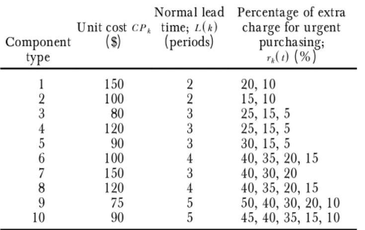
for producing various products, the hourly labour cost at regular time, the hourly labour cost at overtime, and some other cost terms. Table 2 shows the unit cost, nor-mal lead time of each component, and the extra charge of urgent purchasing under various lead time requirements. For example, in the ® rst row, the unit cost of component 1 is $150, its normal lead time is 2 periods, and the extra charge for urgent purchasing is 20% for 0 period lead time, and 10% for 1 period lead time. Here, the 0 period lead time implies that the component should arrive in the current period.
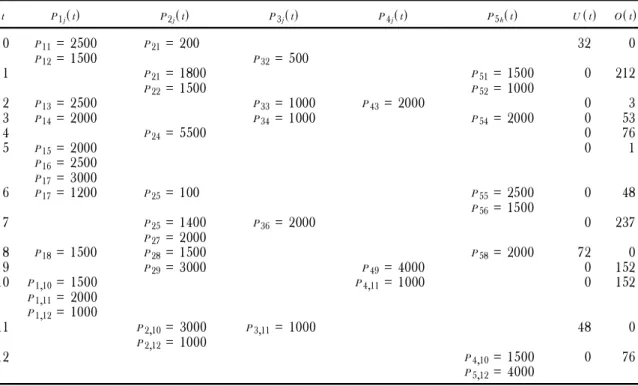
Table 3 shows the relevant data for 12 customer orders. For example, in order 1, three types of products are ordered; their due date is at period 1; its tolerable periods for delayed shipping is 2 periods. The production of these orders has been planned in a current eective MPS ( Table 4) , where a portion of the plan has been executed and the time left is 13 periods ( from t = 0 to
t = 12) . Note that order 4 is to be regarded as a crucial order.
At this point, a rush order arrives which demands 2000 pieces of product 1 ( i.e. R1= 2000) and 1500 pieces of product 2 ( i.e. R2= 1500) . The decision maker wants to know the extra spend involved in producing the rush order under various combinations of production strate-gies. Here, a production strategy implies a set of upper bounds to be imposed on the last three objectives. That is, the last three objectives are modelled as constraints and the ® rst objective is the main objective. The proposed model then becomes a mixed integer linear programming model.
The computation was performed on a PC486 machine through the use of software package LINDO 87. Four illustrated alternatives for justifying the acceptance of 758 M . C . W u and S . Y . C hen
Table 3. Relevant data of customer orders.
Order ID ( j) Product types ordered ( i) Quantities ordered ( Dij) Due date of the order ( dj) ( periods) Tolerable periods for delayed shipping ( nj) ( periods) 1 1 2 5 2500 2000 1500 1 2 2 1 2 3 5 1500 1500 500 1000 1 2 3 1 3 4 2500 1000 2000 2 3 4 1 2 3 5 2000 5500 1000 2000 4 1 5 1 2 5 2000 1500 2500 7 2 6 1 3 5 2500 2000 1500 7 2 7 1 2 15002000 7 2 8 1 2 5 1500 1500 2000 8 1 9 2 4 30004000 9 1 10 1 2 5 1500 3000 1500 12 3 11 1 3 4 2000 1000 1000 12 3 12 1 2 5 1000 1000 4000 12 3
Table 1. Conversion factors for the production of various pro-ducts and relevant cost data.
Product
type Conversionfactors ( Ki)
Manufacturing cost per unit ( P Vi) ( $) Product 1 1´00 1000 Product 2 0´90 600 Product 3 1´10 1500 Product 4 0´60 500 Product 5 0´90 600 Wr= $ 60/man-hour Wo= $ 90/man-hour Cs= $ 6000/setup Ts= 1 hour/setup int= 0´002/period U W= 40´0 hours/man-period U B= 0´10 U W
Table 2. Cost data, normal lead time of components and per-centages of extra charge for their urgent purchasing.
Component type Unit cost C Pk ( $) Normal lead time; L(k) ( periods) Percentage of extra charge for urgent
purchasing; rk(t) ( % ) 1 150 2 20, 10 2 100 2 15, 10 3 80 3 25, 15, 5 4 120 3 25, 15, 5 5 90 3 30, 15, 5 6 100 4 40, 35, 20, 15 7 150 3 40, 30, 20 8 120 4 40, 35, 20, 15 9 75 5 50, 40, 30, 20, 10 10 90 5 45, 40, 35, 15, 10
rush orders were evaluated and the results are shown in Table 5.
In alternative 1, there is no constraint imposed on the last three objectives. The proposed model suggests a new optimum MPS together with the following outcomes. The extra spend due to the production of the rush
order ( Z1) is $125 846. The second objective ( Z2) , back-order of the crucial back-order ( back-order 4) , is 2 000 pieces for product 1 and 222 pieces for product 2. The demand for liquid assets ( Z3) is increased by $119 694. The inventory ( Z4) is increased by $197 354.
Suppose the decision maker requests that the due date
Table 4. The original MPS together with undertime and overtime at each period, where the workforce size is a constant, that is, W (t)= 60.
t P1j(t) P2j(t) P3j(t) P4j(t) P5h(t) U(t) O(t) 0 P11= 2500 P12= 1500 P21= 200 P32= 500 32 0 1 P21= 1800 P22= 1500 P51= 1500 P52= 1000 0 212 2 P13= 2500 P33= 1000 P43= 2000 0 3 3 P14= 2000 P34= 1000 P54= 2000 0 53 4 P24= 5500 0 76 5 P15= 2000 P16= 2500 P17= 3000 0 1 6 P17= 1200 P25= 100 P55= 2500 P56= 1500 0 48 7 P25= 1400 P27= 2000 P36= 2000 0 237 8 P18= 1500 P28= 1500 P58= 2000 72 0 9 P29= 3000 P49= 4000 0 152 10 P1,10= 1500 P1,11= 2000 P1,12= 1000 P4,11= 1000 0 152 11 P2,10= 3000 P2,12= 1000 P3,11= 1000 48 0 12 P4,10= 1500 P5,12= 4000 0 76
Table 5. Justi® cation results for accepting the rush order under various production policies ( main objective is Z1) .
Upper bounds of other objectives
Z1 ( $) Z2 ( pieces) Z3 ( $) Z4 ( $) A1 * 125 846 B14= 2000 B24= 222 B34= 0 B54= 0 119 694 197 354 A2 B14£ 0 B24£ 0 B34£ 0 B54£ 0 136 706 B14= 0 B24= 0 B34= 0 B54= 0 171 612 101 940 A3 B14£ 0 B24£ 0 B34£ 0 B54£ 0 Z3£ 100 000 152 645 B14= 0 B24= 0 B34= 0 B54= 0 100 000 131 324 A4 B14£ 0 B24£ 0 B34£ 0 B54£ 0 Z4£ (1 250 000/12) 142 540 B14= 0 B24= 0 B34= 0 B54= 0 168 084 104 147
of the whole crucial order be strictly met. Then, in alter-native 2, he/she places a constraint on the second objective; that is, the shipping of the crucial order should not be delayed. We can see that now Z1 increases to $136 706, Z3 increases to $171 612, and Z4 decreases to $101 940. Note that we can also request that only a part of the crucial order, rather than the whole order, should be strictly punctual.
By evaluating the results of alternative 2, the decision maker is still not satis® ed and wants to impose more control on the out¯ ow of cash. Therefore, in alternative 3, he/she further constrains that the increase of cash demand ( Z3) should be less than $100 000. We see that now the extra spending for producing the rush order becomes $152 645 ( 21% higher than that in alternative 1) .
Suppose the decision maker pays more attention to the inventory level than to the cash ¯ ow demand. Therefore, in alternative 4, he/she sets up an upper bound on the inventory level and also requests that the crucial order be
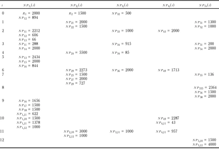
punctually shipped. We see that now Z2 increases to $168 084 ( 68% higher than that in alternative 3) , while Z1 decreases to $142 540 ( 6% lower than that in alternative 3) . The new MPS of this alternative is shown in Table 6.
Other alternatives can be evaluated by placing various constraints on the last three objectives, or on any three objectives by appropriately choosing the main objective. The computed value of Z1 can be a reference for justify-ing the acceptance of the rush order and can help deter-mine the pricing strategy for accepting the rush order.
6. Concluding remarks
This paper presents a multiple criteria decision-making model for justifying the acceptance of rush orders. In justifying the acceptance of rush orders, the MPS has to be replanned by placing the rush order in the immediate production period ( t = 0) . Of the four objectives con-760 M . C . W u and S . Y . C hen
Table 6. The new MPS proposed in alternative 4.
t N P1j(t) N P2j(t) N P3j(t) N P4j(t) N P5h(t) 0 R1= 2000 N P12= 894 R2= 1500 N P32= 500 1 N P21= 2000 N P22= 1500 N PN P5152= 1300= 1000 2 N P11= 2212 N P12= 606 N P13= 66 N P33= 1000 N P43= 2000 3 N P11= 288 N P14= 2000 N P34= 915 N P51= 200 N P54= 2000 4 N P24= 5500 N P34= 85 5 N P13= 2434 N P15= 2000 N P16= 844 6 N P29= 2273 N P36= 2000 N P49= 1713 7 N P25= 1500 N P27= 2000 N P29= 727 N P55= 136 8 N P555= 2364 N P56= 1500 N P58= 2000 9 N P16= 1656 N P17= 1500 N P18= 1500 N P1,11= 622 10 N P1,10= 1500 N P1,11= 1378 N P1,12= 1000 N P49= 2287 N P4,11= 43 11 N P2,10= 3000 N P2,12= 1000 N P3,11= 1000 N P4,11= 957 12 N P5,10= 1500 N P5,12= 4000
cerned, one is taken as the main objective and the other three are described as constraints; the proposed model then becomes a mixed integer programming model for deriving the new optimum MPS.
In planning the new MPS, some notable characteris-tics are discussed below. First, the main objective ( Z1) is modelled on a dierential or increm ental cost basis. That is, we have proposed a method for modelling the extra spend incurred by the new MPS for producing the rush order. In previous literature, replanning of an MPS has generally been performed on a partial total cost basis. That is, such an approach aims to minimize the total cost for producing a new set of orders; however, it generally ignores some cost terms associated with the original MPS. For example, some components which have been committed for production in the original MPS may become idle for some period in the new MPS. The cost of such idleness is generally ignored in the replanning of an MPS because it can only be computed on a di eren-tial basis.
Some extension to this research may be considered. First, the measurement of production objectives may be subjective; in such cases fuzzy mathematics may be included to enhance the model. Second, the assumptions about the production system can further be relaxed or elaborated to accommodate various situations in the real world.
References
Chung, C. H.and Kr aj e w sk i, L. J.,1986, Replanning frequencies for master production schedules. D ecision S cience, 1, 263± 273. De c k r o, R. F. and He r b e r t, J. E., 1984, Goal programming approaches to solve linear decision rules based aggregate production planning models. II E T ransactions, 16, 308± 315. Kr a j e w sk i, L. J. and Rit z ma n, L. P., 1987, O perations
M anag em ent: S trategy and A nalysis( Addison-Wesley, Reading, MA) .
Lin, N. P. and Kr a j e w sk i, L. J., 1992, A model for master
production scheduling in uncertain environments. D ecision
S cience, 1, 839± 861.
Ma sud, S. J. and Hwa ng, C. L.,1980, Aggregate production planning models and application of three multiple objective decision methods. International J ournal of P roduction R esearch, 18, 741± 752.
Na m, S.and Log e nd r a n, R.,1992, Aggregate production plan-ningÐ A survey of models and methodologies. E uropean
J ournal of O perational R esearch, 61, 255± 272.
Ra k e s, T. R., Fr a nz, L. S. and Wy nne, A. J., 1984, Aggregate production planning using chance-constrained goal program-ming. International J ournal of P roduction R esearch, 22, 673± 684. Sr idh a r a n, V. and Be r ry, W. L., 1990, Freezing the master
production schedule under demand uncertainty. D ecision
S cience, 1, 97± 120.
St e ue r, R. E., 1986, M ultiple Criteria O ptimiz ation: T heory,
C om putation, and A pplication( Wiley, New York) .
Ve r c e l l is, C.,1991, Multi-criteria models for capacity analysis
and aggregate planning in manufacturing systems.
I nternational J ournal of P roduction E conomics, 23, 261± 272.