國
立
交
通
大
學
應用數學系
數學建模與科學計算碩士班
碩
士
論
文
Monge-Ampére 方程的數值方法與其在非成像光學上的應用
Numerical Studies on the Monge-Ampére Equation and
its Nonimage Optical Application
研 究 生:蔡玉麟
指導教授:吳金典 教授
Monge-Ampére 方程的數值方法與其在非成像光學上的應用
Numerical Studies on the Monge-Ampére Equation and
its Nonimage Optical Application
研 究 生:蔡玉麟 Student:Yu-Lin Tsai
指導教授:吳金典 Advisor:Chin-Tien Wu
國 立 交 通 大 學
應用數學系數學建模與科學計算碩士班
碩 士 論 文
A ThesisSubmitted to Institute of Mathematical Modeling and Scientific Computing Department of Applied Mathematics
College of Science National Chiao Tung University in partial Fulfillment of the Requirements
for the Degree of Master
in
Mathematical Modeling and Scientific Computing
July 2010
Hsinchu, Taiwan, Republic of China
i
Monge-Ampére 方程的數值方法與其在非成像光學上的應用
學生:
蔡玉麟指導教授
:吳金典國立交通大學應用數學系數學建模與科學計算碩士班
摘
要
本論文介紹光學設計中自由型曲面的設計方法,我們探討了自由型曲面設計
藉由偏微分方程來求得,其中的偏微分方程由 Schruben 推導而來,其偏微分方
程的形式為 Monge-Ampére 方程式,我們考慮簡化型 Monge-Ampére 方程式,藉由
馮教授所使用的方法,加上一個四次微分的消散項,可以使得原來的方程式是一
個完全非線性的方程式轉變成類線性方程式改變了方程式的特性,使得在偏微分
方程上有較好的特性,我們用有限元素法來做為我們的計算方法,挑選 BCIZ 有
限元可以有效的處理四次微分項且並且可以簡單的求得曲面的曲率的計算,也可
以滿足光學系統的所需要的一些特性,只需要解一個線性方程式和使用牛頓疊代
法求做求解用的工具,以獲得較高的計算效率。
ii
Numerical Studies on the Monge-Ampére Equation and
its Nonimage Optical Application
student:
Yu-Lin TsaiAdvisors:Dr. Chin-Tien Wu
Depart of Applied Mathematics
Institute of Mathematical Modeling and Scientific Computing
National Chiao Tung University
ABSTRACT
We consider the freeform surface design problem. Fully nonlinear partial
differential equations as derived by the Schruben for model. The partial differential
equation is the form of well knowMonge-Ampére equation. We following Prof.
Feng’s idea to solve Monge-Ampére equation by adding a vanish moment biharmonic
term. As a result the original fully nonlinear equation is change into quasi-linear
equation. We using finite element method to solve this equation. Its well knows that
the traditional BCIZ element can effectively deal with biharmonic item and compute
the curvature of the solution. Which is usually required in a optical systems. We
descritize the nonlinear equation by the Newton’s method. The numerical studies in
this thesis show that our approach is efficient and accurate.
iLL
誌
謝
本篇論文的完成,首先要感謝我的指導老師-吳金典教授。在老師的指點之下讓我認識了有限元素法、科學 計算和數值偏微分方程等領域,帶領我如何去學習與如何做研究。除了課業之上為我的領路人之外,也讓我學到 了諸多求知與考究數學的方法。在人生上,老師也指點我諸多可為不可為之事,在我人生的道路上為吾樹立了一 個典範,一個值得我效仿的對象。再來我要感謝光電所-田仲豪教授,是帶領我進入光學的世界的導師,為我開 啟了一扇稱之為光學的大門,讓我有深刻的體驗到何謂隔行如隔山,讓我了解了何謂光的世界,給予給我一個碩 士生涯中的研究主題,也是我未來的探討主題,陪我一起悠游光的奧秘這片大海,除了在專業領域上的協助外, 在觀看與了解自然界的本質上也讓我認識到除了數學外的另一種考就方式;而田教授走人生的旅途上讓我見識到 另一種風采,讓我拾取另一副看待人世間的眼鏡。感謝兩位教授讓我在數值計算與光學之間,找到我的興趣與做 研究的方向。除了兩位老師之外,感謝建模所的同學們,陪我度過這兩年給了我許許多多的幫助,在難過的寫程 式的地獄之中也有你們的陪伴,在快樂的研讀之中也不會缺少你們的影子。感謝陳冠羽學長在數值計算上為我指 點迷津,在生活中也給予我相當多的協助;感謝清大資工所徐廷倢同學在寫作程式的給予我許多概念與細節上的 指教,並幫助我思考程式上有新的處理手法;感謝簡明進學長與林至宏同學在光學上為我打起基礎,並不厭其煩 的教導我所不足所缺少的部分,使我能在短時間學習到做研究上所需要最基本的光學知識,為我研究可以順利前 行的兩位前輩。感謝吳恭儉學長以他的偏微分方程的專長在有限元素法的理論部分為我解惑。也要感謝前人所留 下來的許許多多的資料。學生蔡玉麟在此致上我由衷的謝意。 在論文口試的時期,承蒙賴明治教授、田仲豪副教授以及李國明副教授的撥空審閱和提供諸多寶貴意見,令 本論文得以完備與齊全,學生蔡玉麟永銘在心。 除了研究之外,我的生活之中也要感謝蘇偉碩學長、凃芳婷學姊、黃偉強學長、黃喻培學長、段俊旭同學、 陳泓勳同學、碩一的學弟妹們及其田教授實驗室的同學們還有族繁不及備載的其他朋友們。感謝你們跟我在課業 的討論以及努力,也讓我在休閒之刻可以有著充實的時光,交換各式各樣的心得以及意見,在我生活被快樂的時 光所包圍,在互相扶持之下走過這段研究所的日子。 最後,特別感謝我的家人,在他們的支持之下,我才有機會念研究所,在他們的關心與祝福之中,我才有辦 法順利的完成這個里程碑。我願分享這篇論文完成的喜悅與榮耀和我的家人,以及諸位關心我的朋友一同分享。
iv
目
錄
中文提要
………
i
英文提要
………
ii
誌謝
………
iii
目錄
………
iv
Introduction………
1
一、
Mathematical Modeling of Optical design ………
7
二、
Finite Element Method………
15
2.1
Variational formation………
18
2.1.1
Poisson Equation………
18
2.1.2
Biharmonic Equation………
19
2.2
Existence and Uniqueness of Solution………
20
2.3
Estimates for General Finite Element Approximation………
22
2.4
Finite Element Space………
23
2.4.1
Triangular Finite Element………
25
2.5
The Interpolant………
32
2.6
Derive the element matrix………
35
三、
Numerical Method of Monge-Ampére Equation………
36
3.1
Linearization Regularization Monge-Ampére equation…………
36
3.2
Variation formulation………
37
3.3
Non-linear iteration………
37
3.3.1
Fixed-Point Iteration………
38
3.3.2
Newton’s method………
38
3.3.3
Non-linear iteration of regularization Monge-Ampére equation………
38
3.4
Basis function of BCIZ element………
40
3.4.1
The linearization of non-linear term and element matrix………
42
3.4.2
biharmonic term………
43
四、
Numerical Study………
47
4.1
Poisson Equation………
47
4.2
Biharmonic Equation………
50
4.3
Monge-Ampére………
53
五、
Conclusion………
66
References
………
67
Introduction
The Monge-Ampère equation is a important problem in differential geometry,
opti-mal control, mass transportation, geostrophic uid, meteorology and optiopti-mal design [1][2][3][4][5]. In this thesis, we focus on the optical free-form design problem. People study optical
prob-lems for a long time, thank for that the Mathematical fundation of the free-form design is more and more complete, we can try to solve the problem numercally. Now, what's optical free-form design problem? Given a light source and intensity in a optical system, and the illumination distribution on the target plane, the main problem of optical free-form design problem is design a optical system such that the transportantion form the light source to the target plane throught the designed system will not have energy loss. The optical system is generally consisted pf as following re ector amd refractor, etc. .
The general form of Monge-Ampère equation
det(D2u) + F x; u; Du; D2u = 0in (1.1) where D2u = @2u
@xi@xj i;j=1;:::;nis the Hessian of the function u at x 2 .
Suppose coef cients in (1:19) depending on variables x; y; and the unknown function u (x; y) ; (1:19)can be rewritten as following
det(D2u) = auxx+ buxy + cuyy+ (1.2)
The Monge-Ampere equation can be either ellip, parabilic or hyperbolic depending on the sign of 4
4 = + ac + b2 (1.3)
Introduction 2
If 4 > 0, then the Monge-Ampère equation is of elliptic type, if 4 < 0 it is of hyperbolic type and if 4 = 0 it is of parabolic type. A non-linear elliptic partial differential equation. It is well know that the solution of the Monge-Ampère equation is not unique unless we con nes our attention to the convex solutions. The existence and uniqueness of the convex solution of the Monge-Ampére equation satis es version of the maximum principle, and in particular solutions with given Dirichlet condition is proved by Pogorelov in [2, 6] general result on the existence and unquenss are later obtained by Oliker and Wang etc. .
the free-form surface is the solution of Monge-Ampère equation in three dimension space. In 1972 [7], Schruben described the re ector is the solution of the Monge-Ampere equation. He derived the partial differential equation from the integral equation of the en-ergy conservation. In 1993, Oliker and Newman also derived the Monge-Ampere equation in re ector problem. Since the Monge-Ampere equation, a fully non-linear elliptic par-tial differenpar-tial equation, is hard to solve. So if we wanted to use it, we must add some condition such that the equation is more simplify.
until 1990, Benitez , Juan, et al. develoed of the Simltaneous Multiple Surface (SMS) method, for the design of 2D pro les of non-imaging optical devices (SMS2D). It was a breakthrough in a eld dominated by bulky designs. In 2004, SMS non-imaging method generated free-form optical surfaces in 3D (SMS3D) [8], which is a major extension of SMS2D. In the SMS method, the free-form surface is constructed rst by de ning the incoming wavefront and outgoing wavefront, instead of the source and receiver, and then deciding the basic point and optical path length. In order to nd the outgoing wavefront,
Introduction 3
one must solve the Monge-Ampère equation. So, a numerical method is desired for solving the Monge-Ampere equation.
Glowinski, Benamou etc., Gerard Awanou and Feng and Neilan consider the follow-ing Monge-Ampère equation:
det D2u = f in (1.4) u = gon @ (1.5)
where is a convex domain with smooth boundary @ and D2u = uxx uxy
uxy uyy
is the Hessian of the function u at x 2 .
Two method are employed by Benamou, Froese and Oberman [10] to solve the Monge-Ampere equation. One is an explicit nite difference method, The equ (1:4) is using discretized as following standard central difference on a uniform Cartesian grid.
Dxx2 uij Dyy2 uij Dxy2 uij 2 = fij (1.6) where D2xxuij = 1 h2 (ui+1;j+ ui 1;j 2ui;j) D2yyuij = 1
h2 (ui;j+1+ ui;j 1 2ui;j) (1.7)
Dxy2 uij =
1
4h2 (ui+1;j+1+ ui 1;j 1 ui 1;j+1 ui+1;j 1)
The equ (1:6) is further rewrote the a quadratic equation for ui;j;as following
ui;j = 1 2(a1+ a2) 1 2 r (a1 a2)2+ 1 4(a3 a4) 2 + h4f i;j (1.8)
Introduction 4 where a1 = (ui+1;j+ ui 1;j) =2 a2 = (ui;j+1+ ui;j 1) =2 a1 = (ui+1;j+1+ ui 1;j 1) =2 (1.9) a1 = (ui 1;j+1+ ui+1;j 1) =2
The other method employed by Benamou, Froese and Oberman is solving u = T (u) by xed point iteration where
T (u) =4 1 q
(4u)2+ 2 (f det(D2u)) (1.10)
the itervates un+1 = T (un)is obtained by solving
4un+1= q (un xx) 2 + un yy 2 + 2 un xy 2 + 2f (1.11)
Dean and Glowinski [11, 12, 13]. They rst consider the Monge–Ampére equation as a saddle-point problem where a suitable augmented Lagrangian has to he chosen. To solve this saddle-point problem, they advocate an Uzawa–Douglas–Rachford algorithm. The second approach Dean and Glowinski used is to combine non-linear least-square method and operator-splitting. A mixed nite element discretization is used in their formulation.
Feng and Neilan [15, 16] add 42u to regularize the Monge-Ampere equation.
Introduction 5
pde,
42u + det D2u = f; in (1.12) u = gon @ (1.13) 4u = on @ (1.14)
is then separated into coupled second order partial difference equations system
D2u = 0
4tr ( ) + det ( ) = f (1.15)
A mixed nite element is the empolyed to solve the above equations.
Gerard Awanou [30], takes a similar approch as feng and Neilan, by adding n42u
to the Monge-Ampere equation and adding a boundary condition 4u = 2 on @ : The
corresponding variational problem is: to nd u 2 H2( ) ; u = g;
4u = 2 on @ such that Z 4u 4vdx + Z cof D2u Du Dv dx = n Z f vdx 8v 2 H02( ) (1.16) where cof D2u = uyy uxy uxy uxx (1.17)
Again, Awanou employ the mix nite element to approximate the partial differential equa-tion.
In free-form design problem, we must determine the control point and the normal vector. Following this ideal, in this paper, we solve the regularized equ(1:12) which is basically a biharmonic equation with low order nonlinear term, so we solve this regularized
Introduction 6
equation direatly instead of devoupling the equation into a couple low order system as Feng and Neilan did. We employee the Newton iterative method to linearite the nonlinear part, since Newton's method is well known in nding successively better approximations to the zeros of a real-valued nonlinear function. Newton's method can often converge quickly, if the iteration have a good initial point. we choose BCIZ element. BCIZ element is one of the simplest Kirchhoff plate bending elements was presented by Bazeley, Cheung, Irons and Zienkiewicz at the 1965 Wright-Patterson Conference [17]. The “BCIZ element” is named after the authors initials. This element can be derived from the cubic interpolation which basically has 10 degrees of freedom. The variable in the element centroid is condensed out using a kinetic constraint in such a way that the curvature completeness is maintained.
The biharmonic equation, besides providing a benchmark problem for various ana-lytical and numerical methods, arises in many particular applications. For example, the bending behaviour of a thin elastic plane.
Chapter 1
Mathematical Modeling of Optical design
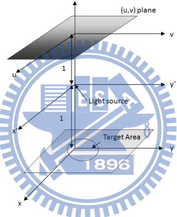
In this chapter, we derive the Monge-Ampére equation follow Schruben in 1972. He consider that a point source though a re ector to target plane, he describing the free-form surface is the solution of Monge-Ampére equation in three dimension space.
The light source is assumed to have some arbitrary directional intensity distribution I and dimensions that emits are negligible compared to the xture size. Distances are normalized such that the distance from the source to the (u; v) plane is unity. The target area on (u; v) plane that is to be illuminated.
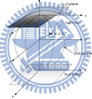
Since the intensity of the source is directional, I may de ned as a function of posi-tion on the unit sphere centered at the source. Spherical coordinates could be used, but it is preferable to employ parametric coordinates (u; v) of the unit sphere. These may be ob-tained as stereographic coordinates, as illustrated in Fig. 1:2, by projecting the unit sphere from its point of tangency to (x; y) plane onto the plane (u; v) plane parallel to (x; y) plane and also tangent to the sphere. The stereographic coordinates of a point on the sphere so projected are the rectangular (u; v) coordinates of the corresponding point on (u; v) plane. De ned a function L = L(x; y), which is the desired pattern of re ected illumination on the target plane. This is de ned as the desired pattern of total illumination at a point (x; y) on the target plane from which has been subtracted the direct illumination of the source at (x; y) which can be obtained directly from the intensity distribution I. by energy
Fig. 1.1. point source of light
1 Mathematical Modeling of Optical design 9 conservation ZZ v( ) L (x; y) dxdy = ZZ I (u; v) d (1.18)
where is solid angles and v ( ) is the target area.
De ne a vector mapping x that maps a point (u; v) on the u; v plane to a vector (light ray) from the orgin (light source) to a point (x0; y0; z0)on the unit sphere.
the explicit form of this map is
x (u; v) = 1 + 1 4w 2 1 u; v; 1 1 4w 2 (1.19)
where w2 = u2 + v2; where the x (u; v) is not unique, under different problem we can
change the coordinate. In 1993, Oliker and Newman proved that the formulation has exis-tence and uniqueness solution.
The differential solid angle d is area on the unit sphere and is related to differential area on the uv plane by the equation
d =jxu xvj dudv (1.20)
Differentiation of equation (1:19) yields
xu(u; v) = 1 + 1 4w 2 2 1 + 1 4v 2 1 4u 2 ; 1 2uv; u (1.21) xv(u; v) = 1 + 1 4w 2 2 1 2uv; 1 + 1 4v 2 1 4u 2 ; v (1.22) therefore d = 1 + 1 4w 2 2 dudv (1.23)
1 Mathematical Modeling of Optical design 10
1 Mathematical Modeling of Optical design 11
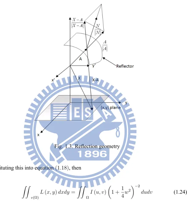
Fig. 1.3. Re ection geometry
Substituting this into equation (1:18), then
ZZ v( ) L (x; y) dxdy = ZZ I (u; v) 1 + 1 4w 2 2 dudv (1.24)
We can describe the re ector by an equation = (u; v) where is the length of a ray with stereographic coordinates (u; v) from the origin to the re ecting surface. We now shall transform the integral equation (1:24) for the re ection function w to a partial differential equation for the surface function .
Let A be a vector with stereographic coordinates (u; v) that strikes the re ector = (u; v). Then A = x, where x is given by Eq. (1:19). Suppose this ray is re ected to the
1 Mathematical Modeling of Optical design 12
point (x; y) on xy plane, then the vector X from the source to this point has the coordinates (x; y; 1)in the x0; y0; z0coordinate system.
The vector N = Au Av is an outward normal vector to the surface = (u; v) at
A. Since A = x, N = (px + xu) (qx + xv) (1.25) where p = uand q = v: We nd N = 2 1 + 1 4w 2 2 x p xu q xv (1.26)
As is illustrated in Figure, the law of re ection requires that
A jAj + A X jX Aj = 2N (A N ) jAj jNj2 (1.27) then X = A +jX Aj x 2N (x N ) =jNj2 (1.28) since A= jAj = x
So the x; y can be show as
x = uG + 2 uF (1.29) y = vG + 2 vF (1.30)
1 Mathematical Modeling of Optical design 13 where G = 1 + 1 4w 2 1 + F " 2 1 + 1 4w 2 2 + 2u+ 2v ( uu + vv) 1 +1 4w 2 1# (1.31) F = 1 + 1 1 4w 2 1 + 1 4w 2 1 1 14w2 h 2 1 + 1 4w2 2 2 u 2v i + 2 ( uu + vv) 1 +14w2 1 (1.32)
The integration over x and y in the left-hand side of (1:24) may be transformed to integration over u and v by multiplication by the Jacobian
D = xu+ ux + uux u+ uvx v
yu+ uy + uuy u+ uvy v
xv + vx + vux u+ vvx v
yv+ vy + vuy u+ vvy v
(1.33)
The a re ector = (u; v) with continuous second derivatives, the integral equation (1:24)is equivalent to the partial differential equation
L (x (u; v; ; u; v) ; y (u; v; ; u; v)) D = I (u; v) 1 +1 4w
2 2
(1.34)
Expanding the jacobian
D = J u v uu vv 2uv + J uv + vJ u uu
+ J vv+ Ju u+ uJ + vJ v uv
+ Ju v + vJ u v vv+ Juv+ uJ v+ vJu (1.35)
where
1 Mathematical Modeling of Optical design 14
The leading term of the differential equation is ( uu vv 2
uv), so it easy to see the
equation is Monge-Ampere type. We consider the ideal case
uu vv 2uv = f (1.37)
Chapter 2
Finite Element Method
The basic idea in any numerical method for a differential equation is to discretize the given continuous problem to obtain a discrete problem or system of equations with only nitely many degrees of freedom such that the differential equation can be solved by using a computer.
Finite element method start from a reformulation of the given differential equation as an equivalent variational problem. In the case of elliptic equations this variational problem in basic case is a minimization problem of the form
F ind u2 V such that F (u) 5 F (v) for all v 2 V (2.38)
where V is a given set of admissible functions and F : V ! R is a functional. F (v) is the total energy associated with v and (2:38) corresponds to an equivalent characterization of the solution of the differential equation as the function in V that minimizes the total energy of the considered system. In general the dimension of V is in nite and thus in general the problem (2:38) can't be solved exactly. To obtain a problem that can be solved on a computer the idea in the nite element method is to replace V by a set Vh consisting
of simple function only depending on nitely many parameters. This leads to a nite-dimensional minimization problem of the form:
F ind uh 2 Vh such that F (uh)5 F (v) for all v 2 Vh (2.39)
2 Finite Element Method 16
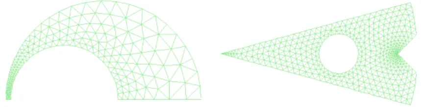
Fig. 2.4. mesh of two dimension domain
This problem is equivalent to a linear or non-linear system of equations. We hope that the solution uhof this problem is suf ciently good approximation of the solution of the original
minimization problem (2:38). Usually one chooses Vh to be a subset of V and in this case
(2:39)corresponds to the classical Ritz-Galerkin method.
To solve a given differential or integral equation approximately using the nite ele-ment method, one has to go through basically the following steps:
1. Variational formulation of the given problem
2. Discretization using FEM: construction of the nite dimensional space Vh
3. Generating Mesh
4. Choose basis function
5. Assembling
2 Finite Element Method 17
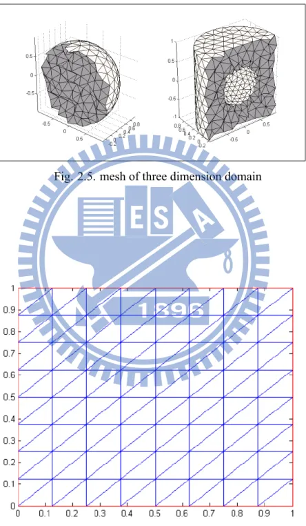
Fig. 2.5. mesh of three dimension domain
2.1 Variational formation 18
2.1 Variational formation
In this section we will give two example for variation formulation. One is Poisson equation, other is biharmonic equation.
2.1.1 Poisson Equation
Consider the following boundary value problem for the Poisson equation, the second order differential equation:
O (AOu) = f in
u = 0 on @ (2.40) where is a bounded open domain in the plane R2with boundary @ ; A is a matrix, f is a
given function and as usual,
u = @
2u
@x2 +
@2u
@y2 (2.41)
A number of problems in physics and mechanics are modelled by (2:40); u may represent for instance a temperature, an electro-magnetic potential or the displacement of an elastic membrane xed at the boundary under a transversal load of intensity f.
We shall now give a variational formulation of problem (2:40) : We shall rst show that if u satis es (2:40) ; then u is the solution of the following variational problem:
Z vO (AOu) dx = Z OvAOudx @u @nvj@ = Z vf dx (2.42)
where v is test function in H1
2.1 Variational formation 19
2.1.2 Biharmonic Equation
Consider the following boundary value problem for the biharmonic equation, the fourth order differential equation: 8
< : 2u = f in u = 0 on @ @u @n = 0 on @ (2.43) where is a bounded open domain in the plane R2 with boundary @ ; f is a given function
and as usual, 42u = @ 4u @x4 + 2 @4u @x2@y2 + @4u @y4 (2.44)
A number of problems in physics and mechanics are modelled by (2:43); u may represent the solution of Stokes ows or the displacement of plane bending problem.
Z v42udx = Z OvO4udx @4u @n vj@ = Z 4v4udx 4u@n@vj@ = Z vf dx (2.45) where v is test function in H2
0( ), v = 0 on @ ; @v
@n = 0on @ .
Case in point, regularization Monge-Ampére equation, it has second order and fourth order differential term. We will introduction it in chapter 3.
2.2 Existence and Uniqueness of Solution 20
2.2 Existence and Uniqueness of Solution
De nition Let H be a Hilbert space. A bilinear form a : H H ! R is called continuous provided there exists C > 0 such that
ja (u; v)j Ckuk kvk for all u; v 2 H
A symmetric continuous bilinear form a is called H-elliptic, or short elliptic or coercive, provided for some > 0,
a (v; v) kvk for all v 2 H
clearly, every H-elliptic bilinear form a induces a norm via
kvka :=
p
a (v; v) (2.46)
This is equivalent to the norm of the Hilbert space H. The norm (2:46) is called the energy norm.
As usual, the space of continuous linear functions on a normed linear space V will be denoted by V0:
Example Consider the boundary value problem of Poisson equation:
O (Ou) = f in
2.2 Existence and Uniqueness of Solution 21
One variational formulation for this is: Take
V = H1( ) a (u; v) =
Z
(Ou Ov) dx (2.48) F (v) = (f; v)
To prove a ( ; ) is continuous, observe that
ja (u; v)j j(u; v)H1j kukH1kvkH1 (2.49)
The Lax-Milgram Theorem Given a Hilbert space (V; ( ; )), a continuous, coercive bilinear form a ( ; ) and a continuous linear functional F 2 V0, there exists a unique u 2 V
such that
2.3 Estimates for General Finite Element Approximation 22
2.3 Estimates for General Finite Element Approximation
Let u be the solution to the variational problem and uhbe the solution to the approximation
problem. To estimate the error ku uhkV :
Céa Lemma Suppose the bilinear form a is V-elliptic with Hm
0 ( ) V Hm( ) :
In addition, suppose u and uh are the solution of the variational problem in V and Vh,
respectively, Then ku uhkV C inf vh2Vhku vhkV (2.51)
2.4 Finite Element Space 23
2.4 Finite Element Space
Finite element have two type, conforming nite element and nonconforming nite element, in the theory of conforming nite element it is assumed that the nite element spaces lie in the function space in which the variational problem is posed. Moreover, we also require that the given bilinear form a ( ; ) can be computed exactly on the nite element spaces. The Finite element space of nonconforming nite element do not lie in function space.
Now we follow Ciarlet's de nition of a nite element (Ciarlet 1978).
De nition Let
1. K Rnbe a bounded closed set with non-empty interior and piecewise smooth
boundary (the element domain),
2. P be a nite-dimensional space of functions on K (the space of shape function) and
3. N = fN1; N2; :::; Nkg be a basis for P0(the set of nodal variable).
Then (K; P; N ) is called a nite element.
De nition Let (K; P; N ) be a nite element. The basis f'1; '2; :::; 'kg of P dual to N is called the nodal basis of P.
After generating Mesh, we construct a nite dimensional subspace Vh of the space
V de ned consisting of piecewise linear function. We now let Vh be the set of functions
2.4 Finite Element Space 24
observe that Vh V:As parameter to describe a function Nj = v (xj)we may choose the
values Nj = v (xj)at the node points xj; j = 0; :::; m + 1: Let us introduction the basis
function j 2 Vh; j = 0; :::; m + 1:de ned by
j(xi) = ij (2.52)
i.e., jis the continuous piecewise linear function that take the value 1 at node point xj and
the value 0 at other node points. A function v 2 Vh then has the representation
v (x) =
m
X
i=1
i i(x) ; x2 (2.53)
where Nj = v (xj), i.e., each Nj = v (xj) can be written in a unique way as a linear
combination of the basis function j: In particular it follow that Vh is a linear space of
dimension m with basis 'j m i=1:
We consider the shape function of K, because we need to compute the solution on computer. We give some example of Finite Element, and how to connect the global coor-dinate with local coorcoor-dinate.
2.4 Finite Element Space 25
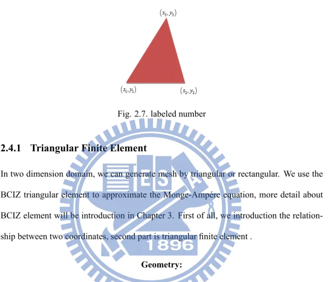
Fig. 2.7. labeled number
2.4.1 Triangular Finite Element
In two dimension domain, we can generate mesh by triangular or rectangular. We use the BCIZ triangular element to approximate the Monge-Ampére equation, more detail about BCIZ element will be introduction in Chapter 3. First of all, we introduction the relation-ship between two coordinates, second part is triangular nite element .
Geometry:
The geometry of the 3-node triangle show in Figure 2.4 is speci ed by the location of its three corner nodes on the fx; yg plane. The nodes are labeled 1, 2, 3 while travers-ing the sides in counterclockwise fashion. The location of the corners is de ned by their coordinates:
(xi; yi) i = 1; 2; 3
the area of triangle is denoted by A and is given by:
2A = det 2 4 x11 x12 x13 y1 y2 y3 3 5 = x21y31 x31y21 (2.54) where xij = xi xj; yij = yi yj for i; j = 1; 2; 3 i 6= j:
2.4 Finite Element Space 26
Properties of Triangular Coordinates:
Consider triangular on regular triangular, points of the triangle may also be located in terms of a parametric coordinate system:
1; 2; 3
this is a local coordinate.
Represent a set of straight lines parallel to the side opposite to the ith corner. See
Figure. The equation of sides 12, 23 and 31 are '1 = 0; '2 = 0and '3 = 0:respectively. The three corners have coordinates (0; 0; 1) ; (0; 1; 0) and (1; 0; 0) :The three midpoints of the sides have coordinates, 1
2; 1 2; 0 ; 0; 1 2; 1 2 and 1 2; 0; 1 2 ;the centroid 1 3; 1 3; 1 3 ;and so
on. The coordinates are not independent because their sum is unity:
2.4 Finite Element Space 27
Coordinate Transformations:
Quantities which are closely linked with the element geometry are naturally ex-pressed in triangular coordinates. On the other hand, quantities such as displacements, strains and stresses are often expressed in the Cartesian system x; y. We therefore need transformation equations through which we can pass from one coordinate system to the other.
Cartesian and triangular coordinates are linked by the relation 2 4 x1 y 3 5 = 2 4 x11 x12 x13 y1 y2 y3 3 5 2 4 12 3 3 5 (2.56)
The rst equation says that the sum of the three coordinates is one. The second and third express x and y linearly as homogeneous forms in the triangular coordinates. These simply apply the linear interpolant formula to the Cartesian coordinates: x = x1 1+ x2 2+ x3 3 and y = y1 1+ y2 2+ y3 3: Inversion of (2:56) yields 2 4 12 3 3 5 = 1 2A 2 4 x2y3 x3y2 y23 x32 x3y1 x1y3 y31 x13 x1y2 x2y1 y12 x21 3 5 2 4 1 x y 3 5 (2.57) Partial Derivatives:
From equations (2:56) and (2:57) we immediately obtain the following relations be-tween partial derivatives:
@x @ i = xi; @y @ i = yi (2.58) @ i @x = yjk 2A; @ i @y = xkj 2A (2.59)
2.4 Finite Element Space 28
where j and k denote the cyclic permutations of i: For example, if i = 3, then j = 1 and k = 2. The rst derivatives of a function w ( 1; 2; 3)with respect to x or y follow immediately from (2:59) and application of the chain rule:
@w @x = 1 2A @w @ 1y23+ @w @ 2y31+ @w @ 3y12 (2.60) @w @y = 1 2A @w @ 1x32+ @w @ 2x13+ @w @ 3x21 (2.61) which matrix form is
@w @x @w @y = 1 2A y23 y31 y12 x32 x13 x21 2 6 4 @w @ 1 @w @ 2 @w @ 3 3 7 5 (2.62)
2.4 Finite Element Space 29
Triangular Finite Element
Let K be any triangle. Let Pk denote the set of all polynomials in two variables of
degree k.
1. Linear Lagrange triangle
Let P = P1. Let N1 =fN1; N2; N3g (dim P1 = 3)Note that “ ” indicates the nodal
Fig. 2.8. Linear Lagrenge triangle
2.4 Finite Element Space 30
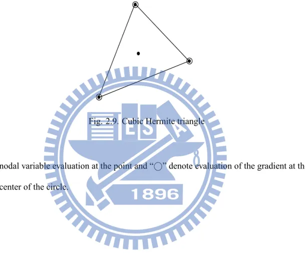
2. Cubic Hermite triangle
Let P = P3. Let N3 = fN1; N2; :::; N10g (dim P3 = 10)Note that “ ” indicates the
Fig. 2.9. Cubic Hermite triangle
nodal variable evaluation at the point and “ ” denote evaluation of the gradient at the center of the circle.
2.4 Finite Element Space 31
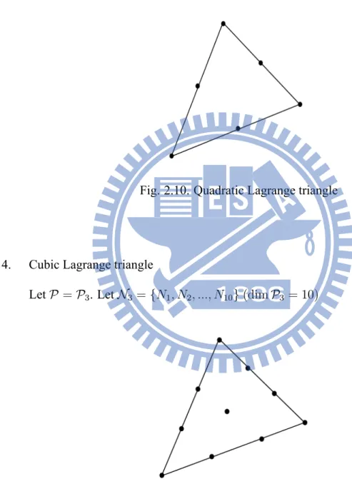
3. Quadratic Lagrange triangle
Let P = P2. Let N2 =fN1; N2; :::; N6g (dim P2 = 6)
Fig. 2.10. Quadratic Lagrange triangle
4. Cubic Lagrange triangle
Let P = P3. Let N3 =fN1; N2; :::; N10g (dim P3 = 10)
2.5 The Interpolant 32
2.5 The Interpolant
Consider a function w (x; y) that varies linearly over the triangle domain. In terms of Cartesian coordinates it may be expressed as
w (x; y) = a0 + a1x + a2y (2.63)
where a0, a1 and a2 are coef cients to be determined from three conditions. In nite
element work such conditions are often the nodal values taken by N at the corners:
N1; N2; N3
The expression in triangular coordinates makes direct use of these three values:
w ('1; '2; '3) = N1'1+ N2'2+ N3'3 = N1 N2 N3 2 4 ''12 '3 3 5 (2.64) = '1 '2 '3 2 4 NN12 N3 3 5
equation (2:64) is called a linear interpolant for w.
De nition Given a nite element (K; P; N ), let the set f'i : 1 i kg P be the
basis dual to N . If v is a function for which all Ni 2 N ; i = 1; :::; k are de ned, then we
de ne the local interpolant by
w (v) :=
k
X
i=1
2.5 The Interpolant 33
Interpolant of Triangular Finite Element
1. Linear Lagrange triangle
'1 = 1 '2 = 2
2.5 The Interpolant 34
2. Cubic Hermite triangle
'1 = 21( 1+ 3 2+ 3 3) 7 1 2 3 '2 = 21(x21 2 x13 3) + (x13 x21) 1 2 3 '3 = 21(y21 2 y13 3) + (y13 y21) 1 2 3 '4 = 22(3 1+ 2+ 3 3) 7 1 2 3 '5 = 22(x32 3 x21 1) + (x21 x32) 1 2 3 '6 = 22(y32 3 y21 1) + (y21 y32) 1 2 3 '7 = 23(3 1+ 3 2+ 3) 7 1 2 3 '8 = 23(x13 1 x32 2) + (x32 x13) 1 2 3 '9 = 23(y13 1 y32 2) + (y32 y13) 1 2 3 '10 = 27 1 2 3 (2.67)
2.6 Derive the element matrix 35
2.6 Derive the element matrix
The variation formulation of Possin equation Z
OvOudx =Z vf dx (2.68)
let fKigi is nonoverlapping triangular domain, and [ n i=1Ki = ;then Z OvOudx = n X i=1 Z ei OvOudx (2.69)
on each element Ki the global coordinate x; y transfor into local 1; 2; 3 the linear
La-grange interpolation of w in the local interpolant w = N1'1+N2'2+N3'3 =
2 4 NN12 N3 3 5 = N ; r = Zr 1; 2; 3;where Z = " @ 1 @x @ 2 @x @ 3 @x @ 1 @y @ 2 @y @ 3 @y # Z ei OvOudx =Z ei Vr TZTZr ; N jJj d 2d 3 (2.70) where 1 = 1 2 3:
the local element matrix isRe
ir ;
TZTZ
Chapter 3
Numerical Method of Monge-Ampére
Equation
We follow the Feng's method, that is adding a vanishing biharmonic term such that the fully non-linear Monge-Ampére equation become regular. The elliptic regularization Monge-Ampére equation:
42u + det D2u = f; in
u = gon @ (3.71) 4u = on @
where is a bound domain in the R2 with a smooth boundary @ , f is a given function
3.1 Linearization Regularization Monge-Ampére equation
the function of regularization Monge-Ampére equation
M A [u] = 42u + det D2u (3.72) variation of MA [u] is
DuM A [u] = (Dyyu) (Dxx) + (Dxxu) (Dyy) 2 (Dxyu) (Dxy) 42
= O cof(D2u)O 42 (3.73) the linearization regularization Monge-Ampére equation
42u +O cof(D2u)Ou = f (3.74)
3.3 Non-linear iteration 37
3.2 Variation formulation
the equivalent variational problem
Z 42u vdx + Z O cof(D2u)Ou vdx = Z f vdxin (3.75) the weak formulation of the biharmonic term R 42u vdxand 4u =
Z 42u vdx = Z @ rv n Z 4u 4vdx = Z @ r nv Z 4u 4vdx = Z 4u 4vdx (3.76)
where v = 0 on @ and the second boundary condition same as 4u = 0 on @ : the weak formulation of the fully non-linear term
Z O cof D2u Ou vdx = Z @ cof D2u Ou nvdx Z cof D2u Ou Ovdx = Z cof D2u Ou Ovdx (3.77) So the equivalent variational problem of equation (3:71) is
Z 4u 4vdx Z cof D2u Ou Ovdx = Z f vdxin (3.78)
3.3 Non-linear iteration
For non-linear problem, we usually use iterative method such as xed-point iteration, Newton's iteration etc.. Iteration method can be classi ed by the rate of convergence, q-quadratically, q-superlinearly, and q-linearly.
3.3 Non-linear iteration 38
3.3.1 Fixed-Point Iteration
Many non-linear equation are naturally formulated as xed-point problem
x = K (x) (3.79)
where K, the xed-point map may be non-linear. A solution ^x of (3:79) called a xed point of the map K. The xed-point iteration is given by
xn+1 = K (xn) (3.80)
This iterative method is also called non-linear Richardson iteration, Picard iteration, or the method of successive substitution.
3.3.2 Newton's method
The Newton's iteration is
xn+1 = xn F0(xn) 1F (xn) (3.81)
sometimes the F0(x
n) 1is not easy to nd, then we can consider use approximate the term,
such as chord method, Shamanskii method or secant method etc..
3.3.3 Non-linear iteration of regularization Monge-Ampére equation
The regularization Monge-Ampére equation
F [u] = f + 42u det D2u (3.82) the DuF [u]is
3.3 Non-linear iteration 39
Newton's iteration of F
3.4 Basis function of BCIZ element 40
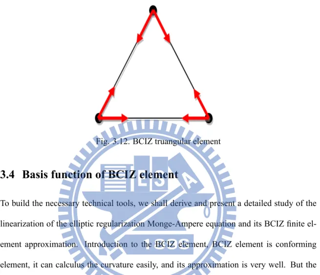
Fig. 3.12. BCIZ truangular element
3.4 Basis function of BCIZ element
To build the necessary technical tools, we shall derive and present a detailed study of the linearization of the elliptic regularization Monge-Ampere equation and its BCIZ nite el-ement approximation. Introduction to the BCIZ elel-ement, BCIZ elel-ement is conforming element, it can calculus the curvature easily, and its approximation is very well. But the basic BCIZ element has a problem, if the mesh is non-uniform mesh, then the numeri-cal result is lost the accuracy. So many people propose the revise BCIZ element such that numerical result has good approximation on non-uniform mesh.
BCIZ element:
Let P = P3. Let N = fN1; N2; :::; N9g
In the free-form design problem, we must to consider that the rst differential of the solution, so we choose BCIZ nite element approximation. It can easy the calculus the rst differential and curve of each element.
3.4 Basis function of BCIZ element 41
The visible degree of freedom of the the element collected in v are
vT = w1 x1 y1 w2 x2 y2 w3 x3 y3 (3.85)
where the xand xis consider rotation, that is different from u, under Cartesian coordinate
u = w; uy = x; ux = y: '1 = 21(3 2 1) + 2 1 2 3 '2 = 21(y12 2+ y13 3) 1 2(y12+ y13) 1 2 3 '3 = 21(x12 2+ x13 3) + 1 2(x12+ x13) 1 2 3 '4 = 22(3 2 2) + 2 1 2 3 '5 = 22(y23 3+ y21 1) 1 2(y23+ y21) 1 2 3 '6 = 22(x23 3+ x21 1) + 1 2(x23+ x21) 1 2 3 '7 = 23(3 2 3) + 2 1 2 3 '8 = 23(y31 1+ y32 2) 1 2(y31+ y32) 1 2 3 '9 = 21(x31 1+ x32 2) + 1 2(x31+ x32) 1 2 3 (3.86) where i are triangular coordinate.
3.4 Basis function of BCIZ element 42
Let
= '1 '2 '3 '4 '5 '6 '7 '8 '9 (3.87) and
w ( 1; 2; 3) = v (3.88) Derive the element matrix Derive the element matrix of the variation equation (3:78) with BCIZ element
3.4.1 The linearization of non-linear term and element matrix
Change coordinate from the global coordinate to the local coordinate, the relationship of Ox;yandO 1; 2; 3 is @w @x @w @y = Z 2 6 4 @w @ 1 @w @ 2 @w @ 3 3 7 5 (3.89) where Z = 1 2A y32 y13 y21 x32 x13 x21 (3.90)
the w use BCIZ element to approximation, w = v
2 6 4 @w @ 1 @w @ 2 @w @ 3 3 7 5 = 2 6 4 @ @ 1 @ @ 2 @ @ 3 3 7 5 v = Bv (3.91)
3.4 Basis function of BCIZ element 43 where B = 2 6 6 6 6 6 6 6 6 6 6 6 6 4 2 1(3 2 1) 2 21+ 2 2 3 2 1 3 2 1( y21 2 y31 3) + 12(y21+ y31) 2 3 2 1y21+ 12(y21+ y31) 1 3 2 1( x21 2 x31 3) 12(x21+ x31) 2 3 2 1x21 12(x21+ x31) 1 3 2 2 3 2 2(3 2 2) 2 22+ 2 1 3 2 2y21+12(y32 y21) 2 3 2 2( y32 3+ y21 1) + 12 (y32 y21) 1 3 2 2x21+ 12( x32+ x21) 2 3 2 2( x32 3+ x21 1) 12(x32 x21) 1 3 2 2 3 2 1 3 2 3y31 12 (y31+ y32) 2 3 2 3y32 12(y31+ y32) 1 3 2 3x31+ 12(x31+ x32) 2 3 2 3x32+12(x31+ x32) 1 3 2 1 2 2 1y31+12(y21+ y31) 1 2 2 1x31 12(x21+ x31) 1 2 2 1 2 2 2y32+12(y32 y21) 1 2 2 2x32 12 (x32 x21) 1 2 2 3(3 2 3) 2 23+ 2 1 2 2 3(y31 1+ y32 2) 12(y31+ y32) 1 2 2 3(x31 1+ x32 2) + 12(x31+ x32) 1 2 3 7 7 7 7 7 7 7 7 7 7 7 7 5 T (3.92)
so theOv = ZBv; then the element matrix of R (cof (D2u)Ou) Ovdx is
Ke1 = Z e BTZTC1ZBjJj d 1d 2 (3.93) where C1is cof (D2u)
3.4.2 biharmonic term
for biharmonic term D 2uwhere D = c 12(1 2) 2 =h @x@22 @2 @y2 2 @2 @x@y i2 4 1 0 1 0 0 0 (12 ) 3 5 2 6 4 @2 @x2 @2 @y2 2@x@y@2 3 7 5 (3.94) Let C2 = 2 4 1 0 1 0 0 0 (12 ) 3 5
3.4 Basis function of BCIZ element 44
The second derivative of a function w ( 1; 2; 3)with respect to x or y from (2:59) and application of the chain rule:
@2w @x2 = 1 2A @ @ 1 @w @xy23+ @ @ 2 @w @xy31+ @ @ 3 @w @xy12 (3.95) = 1 4A2 @2w @ 21y 2 23+ @2w @ 22y 2 31+ @2w @ 23y 2 12+ 2 @2w @ 1@ 2y31y23+ 2 @2w @ 1@ 3y12y23+ 2 @2w @ 2@ 3y12y31 @2w @y2 = 1 2A @ @ 1 @w @yx32+ @ @ 2 @w @yx13+ @ @ 3 @w @yx21 (3.96) = 1 4A2 @2w @ 21x 2 32+ @2w @ 22x 2 13+ @2w @ 23x 2 21+ 2 @2w @ 1@ 2x13x32+ 2 @2w @ 1@ 3x21x32+ 2 @2w @ 2@ 3x21x13 @2w @x@y = 1 2A @ @ 1 @w @yy23+ @ @ 2 @w @yy31+ @ @ 3 @w @yy12 = 1 4A2 @2w @ 21x32y23+ @2w @ 22x13y31+ @2w @ 23x21y12+ @2w @ 1@ 2 (x13y23+ x32y31) + @ 2w @ 1@ 3 (x21y23+ x32y12) + @2w @ 2@ 3 (x21y31+ x13y12) (3.97) which matrix form is
2 6 4 @2w @x2 @2w @y2 2@x@y@2w 3 7 5 = 4A12 2 6 6 6 6 6 4 y2 23 x232 2x32y23 y2 31 x213 2x13y31 y2 12 x221 2x21y12 2y23y31 2x32x13 2 (x32y31+ x13y23) 2y31y12 2x13x21 2 (x13y12+ x21y31) 2y12y23 2x21x32 2 (x21y32+ x32y12) 3 7 7 7 7 7 5 T 2 6 6 6 6 6 6 6 6 6 4 @2w @ 2 1 @2w @ 22 @2w @ 2 3 @2w @ 1@ 2 @2w @ 2@ 3 @2w @ 1@ 3 3 7 7 7 7 7 7 7 7 7 5 (3.98) let S = 1 4A2 2 6 6 6 6 6 4 y2 23 x232 2x32y23 y2 31 x213 2x13y31 y2 12 x221 2x21y12 2y23y31 2x32x13 2 (x32y31+ x13y23) 2y31y12 2x13x21 2 (x13y12+ x21y31) 2y12y23 2x21x32 2 (x21y32+ x32y12) 3 7 7 7 7 7 5 T
3.4 Basis function of BCIZ element 45
the w use BCIZ element to approximation, w = v 2 6 6 6 6 6 6 6 6 6 4 @2w @ 2 1 @2w @ 2 2 @2w @ 23 @2w @ 1@ 2 @2w @ 2@ 3 @2w @ 1@ 3 3 7 7 7 7 7 7 7 7 7 5 = v (3.99) where = 2 6 6 6 6 6 6 6 6 6 6 6 4 6 12 1 0 0 2 3 2y21 2+ 2y31 3 0 0 2y21 1+12(y21+ y31) 3 2x21 2 2x31 3 0 0 2x21 1 12(x21+ x31) 3 0 6 12 2 0 2 3 0 2y32 3 2y21 1 0 2y21 2+12(y32 y21) 3 0 2x32 2+ 2x21 3 0 2x21 2 12(x32 x21) 3 0 0 6 12 3 2 3 0 0 2y31 2 2y32 2 12(y31 y32) 3 0 0 2x31 1+ 2x32 2 12(x31+ x32) 3 2 1 2 2 1 2(y21+ y31) 1 2y31 1+12(y21+ y31) 2 1 2(x21+ x31) 1 2x31 1 12(x21+ x31) 2 2 1 2 2 2y32 2+ 1 2(y32 y21) 1 12(y32 y21) 2 2x32 2 1 2(x32 x21) 1 12(x32 x21) 2 2 1 2 2 2y32 3 1 2(y31 y32) 1 2y31 3 12(y31 y32) 2 2x32 3+1 2(x31+ x32) 1 2x31 3+12 (x31+ x32) 2 3 7 7 7 7 7 7 7 7 7 7 7 5 T (3.100)
so the 4v = S v; then the element matrix of R 4u 4vdx is
Ke2 =
Z T e
TSTC
3.4 Basis function of BCIZ element 46
In this thesis, we will follow this algorithm
1. Given a initial u0, and tolerance T
2. Fixed
3. Newton's iteration if kun+1 un
k T then it converge, if not the iteration is diverge
4. if h2 where h is mesh size then out the algorithm
Chapter 4
Numerical Study
The numerical result will be given, These are three part of this chapter: Poisson equation ,biharmonic equation and Monge-Ampére equation.
4.1 Poisson Equation
Poisson Equation:
4u = f in uj@ = g
where f and g are obtained from a given analytical solution u. We use Linear element and BCIZ element to approximate the Poisson equation. We compute the Poisson equation on different mesh size. Our calculation domain is [0; 1] [0; 1] :The boudary condition are Dirchlet type.
4.1 Poisson Equation 48
4.1.1 Example:
The analytical solution u = ex+y; f = 2ex+y and g = ex+y: we use linear element to
approximate the Poisson equation in this case.
Computed solution uh Error
h ku0 u
hk1 ku0 uhkL2 ku0 uhkH1
1=10 5.97E-03 8.28E-04 2.04E-01 1=20 1.98E-03 2.21E-04 1.02E-01 1=40 6.28E-04 5.68E-05 5.10E-02 1=80 1.91E-04 1.44E-05 2.55E-02 1=160 5.65E-05 3.61E-06 1.28E-02
Table 1. Change of ku uhk w.r.t. h
The convergence rate of L2 norm is second order and H1 norm is rst order. This
result is same as error estimates of the biharmonic equation using BCIZ element approxi-mation.
4.1 Poisson Equation 49
4.1.2 Example:
The analytical solution u = sin (2 x) sin (2 y) ; f = 8 2sin (2 x) sin (2 y)and g = 0:
we use BCIZ element to approximate the Poisson equation in this case.
Computed solution uh Error
h ku0 u
hk1 ku0 uhkL2 ku0 uhkH1
2 3 1.23E-3 8.03E-4 4.37E-2
2 4 1.67E-4 7.54E-5 4.19E-3
2 5 1.32E-5 7.24E-6 5.32E-4
2 6 8.83E-7 7.85E-7 1.18E-4
Table 2. Change of ku uhk w.r.t. h
The convergence rate of L2 norm is third order and H1 norm is second order. This
result is same as error estimates of the biharmonic equation using BCIZ element approxi-mation.
4.2 Biharmonic Equation 50
4.2 Biharmonic Equation
Biharmonic Equation: 42u = f in uj@ = g Ou nj@ = hwhere f, g and h are obtained from a given analytical solution u. We use BCIZ element to approximate the Biharmonic equation. We compute the Biharmonic equation on different mesh size. Our calculation domain is [0; 1] [0; 1] : The boudary condition are Dirichlet type and Neumann type. Because of the Biharmonic equation is fourth order equation, so the approximation of linear element maybe not have a high accuracy.
4.2 Biharmonic Equation 51
4.2.1 Example:
The analytical solution u = x cos(x)ey; f = 0,g = x cos(x)eyandOu = cos(x)ey x sin(x)ey
x cos(x)ey :
Computed solution uh Error
h ku0 u hk1 ku0 uhkL2 ku0 uhkH2 2 2 0.002971694 0.001206162 0.499530706 2 3 0.00065049 0.000273676 0.242128734 2 4 0.000155176 6.32838E-05 0.119339924 2 5 3.78495E-05 1.51706E-05 0.059270777 2 6 9.32505E-06 3.71417E-06 0.02954046 2 7 2.31532E-06 9.1924E-07 0.014747201 Table 3. Change of ku uhk w.r.t. h
The convergence rate of L2 norm is second order and H2 norm is rst order. This
result is same as error estimates of the biharmonic equation using BCIZ element approxi-mation.
4.2 Biharmonic Equation 52
4.2.2 Example:
The analytical solution u = (cos(2 x) 1) (y2 2y3 + y4) ; f = 0,g = x cos(x)ey and
h = 0:
Computed solution uh Error
h ku0 u hk1 ku0 uhkL2 ku0 uhkH2 2 2 0.01171965 0.004154116 0.645238157 2 3 0.004269365 0.001568274 0.307797116 2 4 0.001169401 0.000445123 0.150571686 2 5 0.000302368 0.000116688 0.074556331 2 6 7.67083E-05 2.97733E-05 0.037111559 2 7 1.93091E-05 7.5141E-06 0.018516197 Table 4. Change of ku uhk w.r.t. h
The convergence rate of L2 norm is second order and H2 norm is rst order. This
result is same as error estimates of the biharmonic equation using BCIZ element approxi-mation.
4.3 Monge-Ampére 53
4.3 Monge-Ampére
Regularization Monge-Ampére Equation:
42u + det D2u = f; in u = gon @ 4u = on @
where f and g are obtained from a given analytical solution u. We use BCIZ element to approximate the Monge-Ampére equation. We compute the Poisson equation on different parameter with xed mesh size h. The boudary condition are Dirchlet type. In this section, we provide several 2-D numerical experiments of BCIZ element. And the initial condition is given by zero. The start from 1 to h2:
4.3 Monge-Ampére 54
4.3.1 Example:
This test, we calculus ku0 u
hk for xed mesh size h = 2 8;while varying in order to
approximate ku0 u
k : We use BCIZ element and set to solve problem (3:71) with the analytical solution u = x4+ y2 ; f = 24x2and g = x4+ y2;Our calculation domain is
[0; 1] [0; 1] : solution error ku0 u hk1 ku0 uhkL2 ku0 uhkH2 iter 1 3.05E-1 1.61E-1 5.32 6 2 2 2.30E-1 1.21E-1 4.67 10 2 4 1.13E-1 5.71E-2 3.63 10 2 6 4.23E-2 1.90E-2 2.71 8 2 8 1.45E-2 5.67E-3 1.99 8 2 10 4.50E-3 1.60E-3 1.44 8 2 12 1.29E-3 4.33E-4 1.03 9 2 14 3.48E-4 1.13E-4 7.33E-1 10
Table 5. Change of ku0 u
4.3 Monge-Ampére 55 ku0 u hkL2 ku0 uhkH2 4 p 1 0.160842924 5.319207667 2 2 0.482036757 6.609013597 2 4 0.913779843 7.268095576 2 6 1.218354047 7.670044224 2 8 1.450567862 7.955838131 2 10 1.637202829 8.133261803 2 12 1.772707203 8.235401948 2 14 1.85193153 8.290262971 Table 6. Change of ku0 u hk w.r.t. (h = 2 8)
4.3 Monge-Ampére 56
4.3.2 Example:
This test, we calculus ku0 u
hk for xed mesh size h = 2 8;while varying in order to
approximate ku0 u
k : We use BCIZ element and set to solve problem (3:71) with the analytical solution u = 20x6 + y6 ; f = 18000x4y4 and g = 20x6+ y6;Our calculation
domain is [0; 1] [0; 1] : solution error ku0 uhk1 ku0 uhkL2 ku0 uhkH2 iter 4 6.43 2.88 177.28 5 1 5.22 2.17 167.40 9 2 2 3.31 1.19 148.99 10 2 4 1.79 6.20E-1 125.31 10 2 6 8.72E-1 2.57E-1 101.97 10 2 8 4.02E-1 9.17E-2 82.10 10 2 10 1.80E-1 3.22E-2 65.25 11 2 12 7.93E-2 1.11E-2 51.21 13 2 14 3.45E-2 3.74E-3 39.77 20 Table 7. Change of ku uhk w.r.t. (h = 2 8)
4.3 Monge-Ampére 57 ku0 u hkL2 ku0 uhkH2 4 p 4 0.720510991 125.3567907 1 2.165121991 167.3973101 2 2 4.758836554 210.7002103 2 4 9.926086663 250.6286892 2 6 16.4590354 288.4238466 2 8 23.47587569 328.3874835 2 10 32.93384144 369.1038869 2 12 45.33800541 409.6430813 2 14 61.24535142 449.9969415 Table 8. Change of ku uhk w.r.t. (h = 2 8)
4.3 Monge-Ampére 58
4.3.3 Example:
This test, we calculus ku0 u
hk for xed mesh size h = 2 8;while varying in order to
approximate ku0 u
k : We use BCIZ element and set to solve problem (3:71) with the analytical solution u = ex2+y2
2 ; f = (1 + x2+ y2) ex 2+y2 and g = ex2+y2 2 ;Our calculation domain is [0; 1] [0; 1] : solution error ku0 u hk1 ku0 uhkL2 ku0 uhkH2 iter 1 1.78E-1 1.01E-1 3.03 29 2 2 1.41E-1 8.17E-2 2.72 48 2 4 7.14E-2 4.45E-2 2.13 38 2 6 2.26E-2 1.56E-2 1.57 9 2 8 6.30E-3 4.52E-3 1.13 8 2 10 1.81E-3 1.22E-3 8.00E-1 8
2 12 5.00E-4 3.16E-4 5.67E-1 8 2 14 1.33E-4 8.00E-5 4.01E-1 9
4.3 Monge-Ampére 59 ku0 u hkL2 ku0 uhkH2 4 p 1 0.100518486 3.026105949 2 2 0.32688765 3.840967403 2 4 0.71238757 4.259311736 2 6 0.99970787 4.434163657 2 8 1.157804247 4.506118399 2 10 1.24700059 4.527808719 2 12 1.294427725 4.534697517 2 14 1.309904805 4.53757113 Table 10. Change of ku uhk w.r.t. (h = 2 8)
4.3 Monge-Ampére 60
4.3.4 Example:
This test, we calculus ku0 u
hk for xed mesh size h = 2 8;while varying in order to
approximate ku0 u
k : We use BCIZ element and set to solve problem (3:71) with the analytical solution u = 2p2(x2+y2) 3 4 3 ; f = 1 p x2+y2 and g = 2p2(x2+y2)34 3 ;Our calculation
domain is [0; 1] [0; 1] :Where f has a singular point at (0; 0) :
solution error ku0 u hk1 ku0 uhkL2 ku0 uhkH2 iter 1 1.41E-1 7.89E-2 2.16 5 2 2 1.23E-1 6.93E-2 2.01 19 2 4 7.59E-2 4.48E-2 1.64 9 2 6 2.78E-2 1.81E-2 1.22 10
2 8 8.01E-3 5.57E-3 8.95E-1 8 2 10 2.12E-3 1.55E-3 6.51E-1 8
2 12 5.57E-4 4.08E-4 4.68E-1 9 2 14 1.44E-4 1.04E-4 3.34E-1 11
4.3 Monge-Ampére 61 ku0 u hkL2 ku0 uhkH2 4 p 1 0.078906702 2.164987734 2 2 0.277330363 2.843363264 2 4 0.717285822 3.275360039 2 6 1.15590166 3.442870121 2 8 1.425652095 3.57845558 2 10 1.583580447 3.680240848 2 12 1.671089711 3.747674023 2 14 1.709884392 3.773972909 Table 12. Change of ku uhk w.r.t. (h = 2 8)
4.3 Monge-Ampére 62
4.3.5 Example:
This test, we calculus ku0 u
hk for xed mesh size h = 2 8;while varying in order to
approximate ku0 u
k : We use BCIZ element and set to solve problem (3:71) with the analytical solution u =px2+ y2; f = 0 if (x; y) 6= (0; 0)
? if (x; y) = (0; 0) and g = p
x2+ y2;Our
calculation domain is [ 1; 1] [ 1; 1] :Where f has a singular point at (0; 0), and our guess the value of f at (0; 0) is 3 :
solution error ku0 u hk1 ku0 uhkL2 ku0 uhkH2 iter 1 8.17E-1 6.00E-1 8.65 5 2 2 5.51E-1 3.72E-1 8.82 9 2 4 2.48E-1 1.42E-1 9.27 10 2 6 9.77E-2 5.31E-2 9.72 11 2 8 4.151E-2 2.56E-2 10.09 14 2 10 2.08E-2 1.49E-2 10.32 19 2 12 9.28E-3 6.92E-3 10.51 28 2 13 3.59E-3 1.95E-3 10.66 21 Table 13. Change of ku uhk w.r.t. (h = 1=127)
4.3 Monge-Ampére 63 ku0 u hkL2 ku0 uhkH2 4 p 1 0.599947604 8.652542689 2 2 1.48793695 12.4786026 2 4 2.278636795 18.53711229 2 6 3.398612852 27.50569621 2 8 6.546636298 40.36922514 2 10 15.30464406 58.38278827 2 12 28.35360433 84.08190819 2 13 16.00805235 101.4092367 Table 14. Change of ku uhk w.r.t. (h = 1=127)
4.3 Monge-Ampére 64
Compared with Feng's and Oberman's result: case1: u = ex2+y2 2 ; f = (1 + x2 + y2) ex 2+y2 Ours Feng's ku uhkL2 ku uhkL2 2 1 0.093580805 0:5 0.038717 2 2 0.081721912 0:25 0.040988 2 3 0.064370429 0:1 0.032218 2 4 0.044524223 0:05 0.022259 2 6 0.015620435 0:0125 0.007817 2 9 0.002361013 0:0025 0.001864 2 11 0.00062253 0:0005 0.000405 Ours Oberman's N iter N M1 M2 128 69 121 31965 1205
4.3 Monge-Ampére 65 case 2: u = px2+ y2; f = 0 if (x; y) 6= (0; 0) ? if (x; y) = (0; 0) Ours Feng's ku uhkL2 ku uhkL2 2 1 0.504058 2 2 0.371984 2 3 0.239381 2 4 0.142415 none 2 6 0.053103 2 9 0.014946 2 11 0.001954 Ours Oberman's N iter N M1 M2 128 117 121 36396 10486
Under same accuracy, iteration number is less than other group. And the case have singularty can be achieved with high ef cient computing.
Chapter 5
Conclusion
1. The error of ku uhkL2 of the Monge-Ampére is O ( ) from test cases. The error of
ku uhkH2 of the Monge-Ampére is O (4
p
)from test cases.
2. In numerical simulation of the elliptic regularization Monge-Ampére, the h2;
where h is mesh size.
3. In the singular case, we can shift the grid point such that the singular point locate in a element.
References
[1] L. A. Caffarelli and X. Cabre, “Fully nonlinear elliptic equations,” volume 43 of Amer-ican Mathematical Society Colloquium Publications. AmerAmer-ican Mathematical Society, Providence, RI, 1995.
[2] L. A. Caffarelli and M. Milman, “Monge Ampere Equation: Applications to Geome-try and Optimization, Contemporary Mathematics,” American Mathematical Society, Providence, RI, 1999.
[3] W. H. Fleming and H. M. Soner, “Controlled Markov processes and viscosity solutions,” volume 25 of Stochastic Modelling and Applied Probability. Springer, New York, sec-ond edition, 2006.
[4] D. Gilbarg and N. S. Trudinger, “Elliptic Partial Dierential Equations of Second Order, Classics in Mathematics”, Springer-Verlang, Berlin, 2001. Reprint of the 1998 edition. [5] R. J. McCann and A. M. Oberman. “Exact semi-geostrophic ows in an elliptical ocean
basin,” Nonlinearity,17(5):1891{1922, 2004.
[6] A.V. Pogorelov, "Extrinsic geometry of convex surfaces", AMS, 1973
[7] J. S. Schruben, “Formulation of a Re ector-Design Problem for a Lighting Fixture”, Journal of the Optical Society of America, V.62 N.12 (1972), 1498 1501:
[8] P. Benitez, J. C. Minano, J. Blen, R. Mohedano, J. Chaves, O. Dross, M. Hernandez and W. Falicoff, “ Simultaneous multiple surface optical design methof in three dimen-sions”, Opt. Eng. 43(7) 1489-1502.
[9] C. E. Gutierrez, “The Monge-Ampere Equation,” volume 44, Birkhauser, Boston, MA, 2001.
[10] J. D. Benamou, B. D. Froese and A. D. Oberman, “Two Numerical Method for the Elliptic Monge-Ampere Equation”, Preprint, 2009
[11] E. J. Dean and R. Glowinshi, “Numerical solution of the two-dimensional elliptic Monge–Ampere equation with Dirichlet boundary conditions: an augmented Lagrangian approach”, C. R. Acad. Sci. Paris, Ser. I 336 (2003) 779–784
References 68
[12] E. J. Dean and R. Glowinshi, “Numerical solution of the two-dimensional elliptic Monge–Ampere equation with Dirichlet boundary conditions: a least-squares approach”, C. R. Acad. Sci. Paris, Ser. I 339 (2004) 887–892
[13] E. J. Dean and R. Glowinshi, “Numerical methods for fully nonlinear elliptic equations of the Monge–Ampere type”, Comput. Methods Appl. Mech. Engrg. 195 (2006) 1344– 1386
[14] P. Guan and X.J. Wang “On a Monge-Ampere equation arising in geometric optics”, J. Differential Geom, 48(1998), 205-223
[15] X. Feng and M. Neilan. “Mixed nite element methods for the fully nonlinear
Monge-Amp ere equation based on the vanishing moment method.” SIAM J. Numer. Anal.,47(2),1226-1250, 2009.
[16] X. Feng and M. Neilan. “Vanishing moment method and moment solutions for fully nonlinear second order partial di erential equations.” J. Sci. Comput., 38(1),74-98, 2009.
[17] G. P. Bazeley, Y. K. Cheung, B. M. Irons and O. C. Zienkiewicz, `Triangular ele-ments in plate bendingconforming and non-conforming solutions', Proc. Conf. on Ma-trix Methods in Structural Mechanics, WPAFB, Ohio, 1965. pp. 547-576.
[18] G. A. Mohr and A. S. Power, “Natural Cubic Element Formulation and In nite Domain Modelling for Potential Flow Problems”, ANZIAM J. 45(2003),133-143.
[19] C. A. Felippa and B. Haugen, “From the Individual Element Test to Finite Element Templates: Evolution the Patch test”, International Journal for Numerical Methods in Engineering, Vol. 38, 199-229 (1995)
[20] M. I. G. Bloor and M. J. Wilson, “An approximate analytic solution method for the biharmonic problem”, Proc. R. Soc. A (2006) 462, 1107-1121
[21] Julio Chaves, "Introduction to Nonimaging Optics", CRC, 271-324
[22] P. Benitez and J. C. Minano, “The Future of Illumination Design”, Optics and Photon-ics News, Vol. 18, Issue 5, pp. 20-25
[23] V. Oliker and E. Newman, “The Energy Conservation Equation in the Re ector Map-ping Problem”, Appl. Math. Lett. Vol. 6,No. 1,pp. 91-95, 1993
[24] Daryl L. Logan. “First Course in the Finite Element Method Using Algor”, Pws Pub-lishing, 1997.
References 69
[25] Per-Olof Persson and Gilbert Strang, "A Simple Mesh Generator in MATLAB," SIAM Review Vol. 46 (2) 2004.
[26] C. T. Kelley, “Iterative Method for Linear and nonlinear Equations”, SIAM, Philadel-phia, 1995
[27] D. Braess, “Finite element” , Cambridge University Press, 2001
[28] C. Johnson, “Numerical solution of partial differential equations by the nite element method”, Cambridge University Press, 1988
[29] Susanne C. Brenner and L. Ridgway Scott, “The Mathematical Theory of Finite Ele-ment Methods”, Springer, 2002
[30] G. Awanou “Numerical Methods for Fully Nonlinear Elliptic Equations”, International Conference on Approximation Theory, 2010