多輸入輸出正交分頻多工系統中峰均功率比的減低

國立交通大學

電子工程學系 電子研究所

碩士論文

多輸入輸出正交分頻多工系統中峰均功率

比的減低

On Peak-to-Average Power Ratio Reduction in the

MIMO-OFDM system

研究生：郭彥志

指導教授：桑梓賢 教授

多輸入輸出正交分頻多工系統中峰均功率比的減低

On Peak-to-Average Power Ratio Reduction in the

OFDM system

研 究 生：郭彥志

Student：Yen-Chin Kuo

指導教授：桑梓賢

Advisor：Tzu-Hsien Sang

國 立 交 通 大 學

電子工程學系 電子研究所

碩 士 論 文

A Thesis

Submitted to Department of Electronics Engineering & Institute of Electronics College of Electrical Engineering and Computer Engineering

National Chiao Tung University in partial Fulfillment of the Requirements

for the Degree of Master in Electronics Engineering

August 2006

Hsinchu, Taiwan, Republic of China

多輸入輸出正交分頻多工中峰均功率比的減低

研究生： 郭彥志

指導教授： 桑梓賢

國立交通大學

電子工程學系 電子研究所碩士班

摘要

這篇論文是考慮在正交多頻分工(OFDM)系統中所傳送信號有著令

人討厭的高峰均功率比的問題。在多輸入輸出正交多頻分工( MIMO-OFDM)

系統中，因為多根傳送天線，處理峰均功率比的低複雜度架構是很重要

的。在眾多降低峰均功率比的方法中，選擇對應法( SLM )是有著相對較

高的降低峰均功率比的能力，但同時也有著較高的複雜度和需要傳送額外

訊息的缺點。這篇論文中，結合了低複雜度的 SLM 和傳送額外訊息，模擬

顯示他能有效地降低峰均功率比。並將使用多輸入輸出正交分頻多工系統

的 802.11n 規格實作在 DSP 板上，數據表示出在系統中這架構的確有著很

低的時間複雜度。

On Peak-to-Average Power Ratio Reduction in the OFDM

system

研 究 生：郭彥志 student：Yen-Chih Kuo

指導教授：桑梓賢 Advisors：Tzu-Hsien Sang

Department of Electronics Engineering & Institute of Electronics

National Chiao Tung University

ABSTRACT

This thesis considers the Orthogonal Frequency Division Multiplexing

(OFDM) system’s undesirable feature of a large peak-to-average power ratio

(PAPR) of the transmitted signal. In the MIMO-OFDM system, a low

complexity structure to deal with PAPR problem is important because

multiple transmitter. In the various PAPR reduction methods, the method

selected mapping has high PAPR reduction capability but also high

complexity and needs to transmit additional side information. In this thesis,

we combine low complexity SLM structure and transmitting the side

information, simulation display this method can reduce PAPR effectively.

And implement to DSP board using 802.11n which is MIMO-OFDM system,

profiling that this structure has low complexity and doesn’t engage much time

in the system.

誌謝

兩年的研究所生活一下就過去了。然而在這短短的兩年，卻學到了很

多東西，也有很多收穫。首先這都要謝謝我的指導教授桑梓賢老師，這兩

年之中老師對我的研究給予了相當多的建議與指導，讓我可以順利完成畢

業論文。除此之外，老師也常常與我們分享他對許多事情的觀點與看法，

讓我增長了許多專業領域外的知識。在此還是要再次的謝謝老師。

另外，我也要感謝欣德學長在這兩年之中對我的幫忙。在與他的討論

當中我解決了許多研究上遇到的難題，並且學到很多經驗。當然，也要謝

謝實驗室其他的學長以及同學們，很高興能認識你們，跟你們一起合作。

由於有各位的幫忙，讓我過了兩年充實的研究生生活。

最後，感謝我的家人和朋友在這兩年對我的幫忙和支持，謝謝！

Contents

Chapter 1 Introduction... 9

1.1 PAPR Reduction Scheme... 11

1.1.1 Direct clipping ... 11

1.1.2 Block coding ... 11

1.1.3 Partial Transmit Sequence (PTS) ... 12

1.1.3 Selected Mapping (SLM)... 14

1.1.4 tone injection (TI) ... 15

1.1.5 Tone reservation (TR) ... 16

1.2 A Low Complexity SLM with conversion matrix[13]... 17

Chapter 2 The Brief of EWC PHY Specification For 802.11n ... 20

2.1 PLCP Packet Format ... 20

2.2 Operating Mode ... 21

2.3 Modulation and Coding Scheme(MCS)... 22

2.4 Transmitter Block Diagram... 25

2.5 Timing Parameter... 26

Chapter 3 The Brief of Innovative Quixote DSP Board ... 28

3.1 About Quixote... 28

3.2 Support libraries... 29

Chapter 4 Developing A DSP Program ... 32

4.1 A recommended flow of developing a DSP program ... 32

4.2 Analyzing the C code performance... 33

4.3 Refine the C/C++ code ... 34

4.3.1 Using the intrinsic to replace complicated C/C++ code ... 34

4.3.2 Loop Unrolling... 35

4.3.2 Word access to the packed data... 36

4.3.2 Using compiler option... 36

4.3 Write linear assembly code ... 37

Chapter 5 DSP Board Implementation Result and Discussion... 39

5.1 Choose M = 4 in SLM structure ... 39

5.2 The use of the conversion matrix... 40

5.3 About insert the side information... 41

5.3 Fixed point format on the DSP board ... 42

5.4 About using the digital IO... 44

5.5 The estimate of speeding up the program using FPGA ... 46

Chapter 6 Conclusion ... 49

Chapter 7 Reference ... 50

LIST OF TABLES

Table 01 PAPR of the possible four subcarrier OFDM symbol... 12

Table 02 rate dependent parameters for mandatory 20 MHz, Nss =1 (NES = 1) modes 23 Table 03 rate dependent parameters for mandatory 20 MHz, Nss =2 (NES = 1) modes 23 Table 04 rate dependent parameters for mandatory 20 MHz, Nss =3 (NES =2) modes 23 Table 05 rate dependent parameters for mandatory 20 MHz, Nss =4 (NES = 2) modes 24 Table 06 C compiler intrinsic... 34

Table 07 some common linear assembler’s Directive ... 37

Table 08 computation complexity between IFFT band and conversion matrix ... 41

Table 09 simulation EVM result... 43

Table 10 execute time and bit rate ... 44

LIST OF FIGURES

Figure 01 the PAPR when the difference FFT length ... 10

Figure 02 A block diagram of PTS... 13

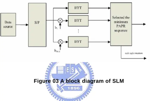
Figure 03 A block diagram of SLM ... 14

Figure 04 CCDF of PAPR of the OFDM system using PTS and SLM method [12] ... 15

Figure 05 A block diagram of TR ... 16

Figure 06 Equivalent SLM with conversion matrix diagram... 18

Figure 07 PLCP packet format ... 20

Figure 08 Transmitter diagram... 25

Figure 09 A flow of developing a DSP program ... 33

Figure 10 A example to show the executing time ... 34

Figure 11 A example to show the loop unrolling ... 35

Figure 12 A example to show word access to packed data ... 36

Figure 13 A example to show a C callable function writing by linear assembly ... 38

Figure 14 CCDF of PAPR in 64-pt FFT length SLM with different M ... 39

Figure 15 The CCDF of PAPR comparison between IFFT bank and conversion matrix 40 Figure 16 SLM structure with transmitting the side information... 42

Figure 17 the percentage of the all block execution time... 44

Chapter 1

Introduction

Orthogonal Frequency Division Multiplexing (OFDM) is an attractive multicarrier transmission technique for different communication application due to its strong immunity to multipath fading and high spectral efficiency comparing with the single carrier system. However, OFDM systems have an undesirable feature of a large peak-to-average power ratio (PAPR) of the transmitted signal. Because OFDM symbol introduces large amplitude variation in time, which can result in nonlinear distortion are introduced in the nonlinear region of high power amplifier (HPA). Nonlinearity will cause intermodulation interference among subcarriers and out-of-band radiation, and finally result in degradation of the bit error rate (BER) and interfere with other system using the adjacent frequency band. Therefore, HPA with a large linear range are required for OFDM systems to avoid above nonlinear effect, but it is a major cost component in OFDM system. Consequently, reducing the PAPR is also reducing the expense of the OFDM systems.

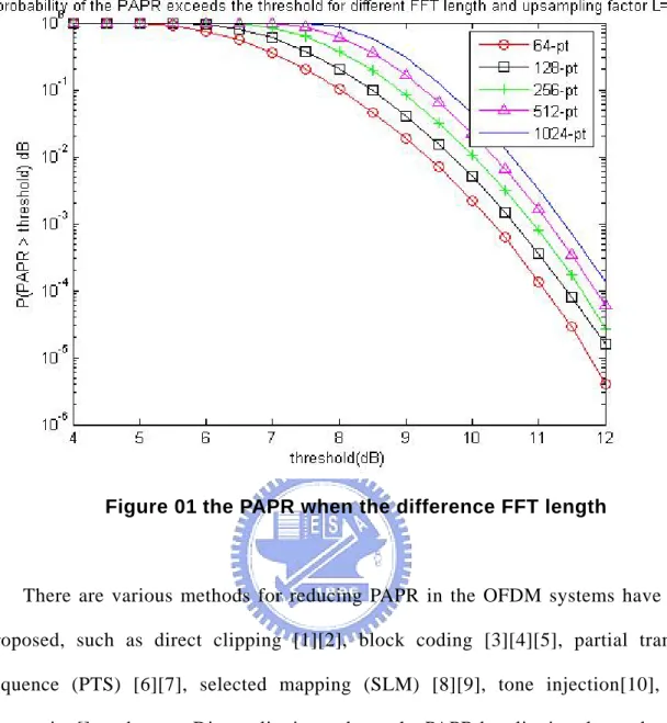
Moreover, PAPR is larger when the FFT length which the OFDM system used is larger. So, as the FFT length is increase, PAPR problem is more critical. Fig1 shows the PAPR vs FFT length relation.

Figure 01 the PAPR when the difference FFT length

There are various methods for reducing PAPR in the OFDM systems have been proposed, such as direct clipping [1][2], block coding [3][4][5], partial transmit sequence (PTS) [6][7], selected mapping (SLM) [8][9], tone injection[10], tone reservation[], and so on. Direct clipping reduces the PAPR by clipping the peak power to one predetermined threshold before entering the nonlinear amplification. Block coding reduces the PAPR by coding the input data to the code word which has low PAPR.The SLM and PTS are the methods that control the phase of the OFDM symbol to reduce PAPR. SLM multiplies the incoming data by several phase sequences at the same time and the data sequence with the lowest PAPR among them is selected to transmit. PTS divides the incoming data into several clusters and optimum rotation factors (or combining sequences) are multiplied to lower the PAPR..

1.1 PAPR Reduction Scheme

1.1.1 Direct clipping

The simplest method to reduce the PAPR is to clip the peak above a certain prescribed level in front of the nonlinear HPA.

The transmitted signal is clipped at amplitude A as follows: -A ( if x < -A ) x ( if A < x < A ) -A ( if A < x ) y ⎧ ⎫ ⎪ = ⎨ ⎪ ⎪ ⎩ ⎭ ⎪ ⎬ ( 1.1 )

where x denotes the signal before clipping and y denotes the signal after clipping.

Since the probability of the occurrence of the high peak power is low, clipping is effective for reducing the PAPR. However, clipping is the nonlinear operation, so it causes the in-band distortion, which results in the BER degradation, and the out-of-band emission, which results in the interference to the adjacent channels in that system’s band and the interference to the other systems using the adjacent frequency band (ACI). Filtering after clipping can reduce the out-of-band emission but may also cause some peak regrowth. Thus, although clipping can be performed easily, its degradation of the BER is large.

1.1.2 Block coding

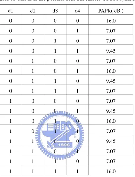
The method of the coding is stated that the desired data sequence is embedded in a larger sequence, and then this mapping is one-to-one and only mapping to a subset of those larger sequences which have lower PAPR. For example, the PAPR of the four subcarriers OFDM system with BPSK modulation are shown in Table 1.

Table 01 PAPR of the possible four subcarrier OFDM symbol d1 d2 d3 d4 PAPR( dB ) 0 0 0 0 16.0 0 0 0 1 7.07 0 0 1 0 7.07 0 0 1 1 9.45 0 1 0 0 7.07 0 1 0 1 16.0 0 1 1 0 9.45 0 1 1 1 7.07 1 0 0 0 7.07 1 0 0 1 9.45 1 0 1 0 16.0 1 0 1 1 7.07 1 1 0 0 9.45 1 1 0 1 7.07 1 1 1 0 7.07 1 1 1 1 16.0

So, if we map a sequence with length 3 to a sequence with length 4, we can choose 8 symbols with low PAPR from the original 16 symbols. And then, as the above table shown, we can reduce PAPR from 16 to 7.07. Unfortunately, the method of the block coding generally decrease data rate hard.

1.1.3 Partial Transmit Sequence (PTS)

The method of the Partial Transmit Sequence (PTS) is stated that the OFDM symbol is partitioned into M disjoint sub-block and then multiplies a M-tuple phase

rotate vector to minimized this OFDM symbol’s PAPR. The phase rotate vector is produced by passing the OFDM symbol into a phase rotate optimizer. A block diagram of Partial Transmit Sequence (PTS) is shown in Fig 1.

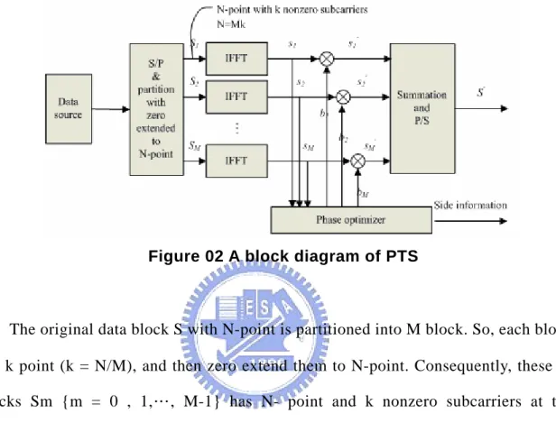
Figure 02 A block diagram of PTS

The original data block S with N-point is partitioned into M block. So, each block has k point (k = N/M), and then zero extend them to N-point. Consequently, these M blocks Sm {m = 0 , 1,…, M-1} has N- point and k nonzero subcarriers at the corresponding position. The objective of the method PTS is to choose bm to make a weighted combination of the M blocks S’ having a low PAPR.

m 1

'

S

M m m

S

b

=

=

∑

( 1.2 ) Where bm {m = 0 , 1,…, M-1} are the weighting vector and are assumed to be pure rotation, usually be called phase rotate vector at this situation. The phase rotate vector must be transmitted to the receiver as side information to recover the received data, and it is result in some loss of the transmission efficiency.

1.1.3 Selected Mapping (SLM)

In the selected mapping, the M – 1 statistically independent phase sequence are generated for multiplying the symbol sequence before the IFFT process. Containing with the symbol sequence itself, there are M difference sequence sent to the IFFT input, and choose one with the lowest PAPR to transmit. A block diagram of Selected Mapping (SLM) is shown in Fig 2.

Figure 03 A block diagram of SLM

The same as the PTS method, the receiver in the SLM method also has to recover data by the side information about which sequence is chosen to multiply the symbol sequence. In the SLM method, when using U-1 statistically independent phase and U kinds of signal totally to select lowest PAPR , we need transmit bit side information. In the PTS method, if we partition the original signal to W parts and use J kinds of rotate phase tune these part block, we need

2

log U

( 1)

2

log W J− _{bit side information.}

Fig4 shows The comparison between PTS and SLM’ s performance to how many side information to need to transmit additionally. We can see that the SLM can reduce the PAPR more than the PTS at the same amount of side information. This is because in the PTS we rotate the phase by clusters, whereas in the SLM we rotate the phase by

one subcarrier. Thus, the probability of low PAPR using the SLM is higher than the PTS.

Figure 04 CCDF of PAPR of the OFDM system using PTS and SLM method [12]

1.1.4 tone injection (TI)

The basic idea of tone injection scheme is to increase the constellation size so that each original constellation points can be mapped to several equivalent points in the expand constellation. Since one data symbol has many usable constellation points to choose, the additionally degrees of freedom can be exploit for reducing PAPR.

This method is called tone injection because substituting a point in the original basic constellation for a new point in the new larger constellation is equivalent to

injecting a tone of the appropriate frequency and phase in the multicarrier signal system.

Tone injection technique has many advantages like it introduces no distortion and no need to exchange side information between transmitter and receiver. However, there is an increase in transmit signal power due to inject signal in the TI technique.

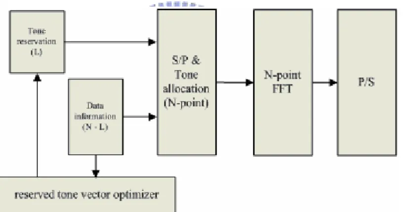
1.1.5 Tone reservation (TR)

In the tone reservation scheme, some of subcarriers in the OFDM system are reserved. These reserved subcarriers don’t carry any data information, and are only for reducing PAPR so as to be also called peak reduction tones.

Figure 05 A block diagram of TR

The peak which the data bears will be detected by reserved tone vector optimizer which generate tone vector to mitigate the peak. Obviously, tone reservation scheme will degrade capacity but it has advantages of low complexity and no overhead on the receiver side comparing other PAPR reduction scheme.

1.2 A Low Complexity SLM with conversion matrix[13]

In the variety of PAPR reduction technique, selected mapping (SLM) approach has a high reduction performance, but it suffer from high computational complexity due to the use of the bank of inverse fast Fourier transforms (IFFT) . So, in this chapter, it focuses on reducing the complexity within SLM.

To make short of the matter, SLM is stated that it has M-1 statically independent sequence to multiply the original data sequence and pass into the IFFT, and then choose one lowest PAPR sequence to transmit. The block diagram of SLM is Fig 2 in chap 1.

At first, we define the data sequence vector

.It is multiplied by a phase rotation vector defined as ( i = 1~M-1) to generate M-1 different output signal . We can write as 0 1 1 [ , ,..., ]T N X X X ₋ = X ( ) ( ) ( ) 0 1 1 [ i , i ,..., i N ] i= B B B − B T T ( ) ( ) ( ) ( ) ( ) ( ) 0 1 1 0 ₀ 1 ₁ 1 ₁ [ i , i ,..., i ]T [ i , i ,..., i ] N N _N i= S S S − = b X b X b −X ₋ S i = iX S R , where ( ) 0 ( ) 0 ( ) 1 ... 0 0 ... i i i N b b Ri b − ⎡ ⎤ ⎢ ⎥ ⎢ ⎥ = ⎢ ⎥ ⎢ ⎥ ⎢ ⎥ ⎣ ⎦ % ( 1.2 )

is phase rotation matrix generate by putting phase rotation vector Bi on its diagonal

line.

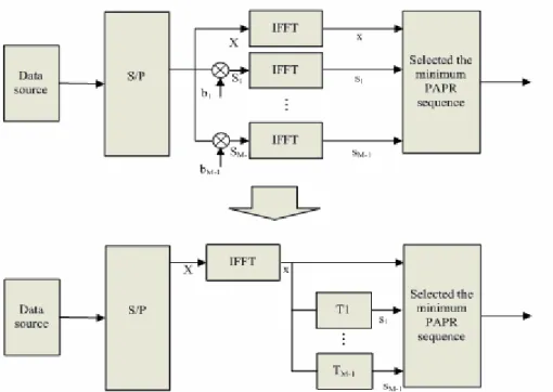
The conversion matrix method is stated that we do not need so many IFFT as to have high complexity if we can transform the action multiplying the phase rotate vector to passing into the conversion matrix.

Figure 06 Equivalent SLM with conversion matrix diagram

We can generate one output signal si by the original IFFT out signal x. Because signal

x and si is { } x=IFFT X =QX ( 4.1) { } i i i s =IFFT S =QS =QR X_i ( 4.2)

Where Q is the IFFT matrix. From (4.1), we have X =Q x−1 , where Q−1 is equivalent to FFT matrix. Then we can obtain

1

i i

s =QR Q x− ( 4.3)

Therefore, the conversion matrix T is represent as T = QRiQ-1

In general, this conversion does not necessarily have low complexity comparing with the original SLM structure. But if we choose the phase rotate vector with care, we can make the conversion matrix have a simple form so as to only need addition

operation but not multiply operation. For example, at the 16-points FFT length case and phase rotate vector is of the form [ 1 , j , 1 , -j , 1 , j , 1 , -j , 1 , j , 1 , -j , … ], the conversion matrix T is like this

1 0 0 0 1 0 0 0 1 0 0 0 -1 0 0 0 0 1 0 0 0 1 0 0 0 1 0 0 0 -1 0 0 0 0 1 0 0 0 1 0 0 0 1 0 0 0 -1 0 0 0 0 1 0 0 0 1 0 0 0 1 0 0 0 -1 -1 0 0 0 1 0 0 0 1 0 0 0 1 0 0 0 0 -1 0 0 0 1 0 0 0 1 0 0 0 1 0 0 0 0 .5 * T = 0 -1 0 0 0 1 0 0 0 1 0 0 0 1 0 0 0 0 -1 0 0 0 1 0 0 0 1 0 0 0 1 1 0 0 0 -1 0 0 0 1 0 0 0 1 0 0 0 0 1 0 0 0 -1 0 0 0 1 0 0 0 1 0 0 0 0 1 0 0 0 -1 0 0 0 1 0 0 0 1 0 0 0 0 1 0 0 0 -1 0 0 0 1 0 0 0 1 1 0 0 0 1 0 0 0 -1 0 0 0 1 0 0 0 0 1 0 0 0 1 0 0 0 -1 0 0 0 1 0 0 0 0 1 0 0 0 1 0 0 0 -1 0 0 0 1 0 0 0 0 1 0 0 0 1 0 0 0 -1 0 0 0 1 ⎡ ⎤ ⎢ ⎥ ⎢ ⎥ ⎢ ⎥ ⎢ ⎥ ⎢ ⎥ ⎢ ⎥ ⎢ ⎥ ⎢ ⎥ ⎢ ⎥ ⎢ ⎥ ⎢ ⎥ ⎢ ⎥ ⎢ ⎥ ⎢ ⎥ ⎢ ⎥ ⎢ ⎥ ⎢ ⎥ ⎢ ⎥ ⎢ ⎥ ⎢ ⎥ ⎢ ⎥ ⎢ ⎥ ⎢ ⎥ ⎢ ⎥ ⎣ ⎦

Chapter 2

The Brief of EWC PHY Specification For 802.11n

This document [14] specifies those features of a device that are necessary to achieve interoperability. It specifies the signals that may be transmitted by the device and received by the device's receivers. This device is referred to as an HT (High Throughput) device. The HT device is assumed to be compliant with 802.11a/b/g/j standards. This document describes the extensions needed in the physical layer for high throughput transmission.

2.1 PLCP Packet Format

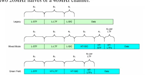
Two new formats are defined for the PLCP (PHY Layer Convergence Protocol): Mixed mode and Green Field. These two formats are called HT formats. Figure

1 shows the legacy format and the HT formats. In addition to the HT formats, there is a legacy duplicate format (specified in section 4.8) that duplicates the 20MHz legacy packet in two 20MHz halves of a 40MHz channel.

The elements of the PCLP packet are: L-STF: Legacy Short Training Field L-LTF: Legacy Long Training Field L-SIG: Legacy Signal Field

HT-SIG: High Throughput Signal Field

HT-STF: High Throughput Short Training Field HT-LTF1: First High Throughput Long Training Field

HT-LTF's: Additional High Throughput Long Training Fields

Data – The data field includes the PSDU (PHY sub-layer Service Data Unit)

The HT-SIG, HT-STF and HT-LTF's exist only in HT packets. In legacy and 12 legacy duplicate formats only the L-STF, L-LTF, L-SIG and Data fields exist.

2.2 Operating Mode

The PHY will operate in one of 3 modes –

z Legacy Mode – in this mode packets are transmitted in the legacy 802.11a/g format.

z Mixed Mode – in this mode packets are transmitted with a preamble compatible with the legacy 802.11a/g – the legacy Short Training Field (STF), the legacy Long Training Field (LTF) and the legacy signal field are transmitted so they can be decoded by legacy 802.11a/g devices. The rest of the packet has a new format. In this mode the receiver shall be able to decode both the Mixed Mode packets and legacy packets.

legacy compatible part. This mode is optional. In this mode the receiver shall be able to decode both Green Field mode packets, Mixed Mode packets and legacy format packets.

The operation of PHY in the frequency domain is divided to the following modes:

z LM – Legacy Mode – equivalent to 802.11a/g

z HT-Mode – In HT mode the device operates in either 40MHz bandwidth or 20MHz bandwidth and with one to four spatial streams. This mode includes the HT-duplicate mode.

z Duplicate Legacy Mode – in this mode the device operates in a 40MHz channel composed of two adjacent 20MHz channel. The packets to be sent are in the legacy 11a format in each of the 20MHz channels. To reduce the PAPR the upper channel (higher frequency) is rotated by 90º relative to the lower channel.

z 40 MHz Upper Mode – used to transmit a legacy or HT packet in the upper 20MHz channel of a 40MHz channel.

z 40 MHz Lower Mode – used to transmit a legacy or HT packet in the lower 20MHz channel of a 40MHz channel

LM is mandatory and HT-Mode for 1 and 2 spatial streams are also mandatory.

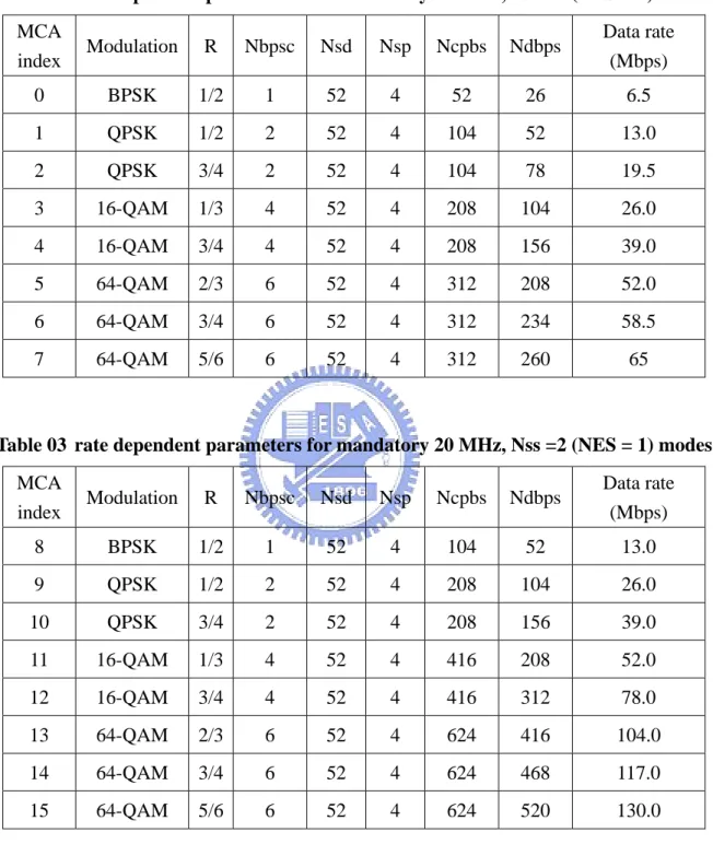
2.3 Modulation and Coding Scheme(MCS)

The Modulation and Coding Scheme (MCS) is a value that determines the modulation, coding and number of spatial channels. It is a compact representation that is carried in the high throughput signal field.

Rate dependent parameters for the full set of modulation and coding schemes (MCS) are shown in Appendix A in Tables 2 to 5. These tables give rate dependent

parameters for MCSs with indices 0 through 31 for 20MHz.

Table 02 rate dependent parameters for mandatory 20 MHz, Nss =1 (NES = 1) modes MCA index Modulation R Nbpsc Nsd Nsp Ncpbs Ndbps Data rate (Mbps) 0 BPSK 1/2 1 52 4 52 26 6.5 1 QPSK 1/2 2 52 4 104 52 13.0 2 QPSK 3/4 2 52 4 104 78 19.5 3 16-QAM 1/3 4 52 4 208 104 26.0 4 16-QAM 3/4 4 52 4 208 156 39.0 5 64-QAM 2/3 6 52 4 312 208 52.0 6 64-QAM 3/4 6 52 4 312 234 58.5 7 64-QAM 5/6 6 52 4 312 260 65

Table 03 rate dependent parameters for mandatory 20 MHz, Nss =2 (NES = 1) modes MCA index Modulation R Nbpsc Nsd Nsp Ncpbs Ndbps Data rate (Mbps) 8 BPSK 1/2 1 52 4 104 52 13.0 9 QPSK 1/2 2 52 4 208 104 26.0 10 QPSK 3/4 2 52 4 208 156 39.0 11 16-QAM 1/3 4 52 4 416 208 52.0 12 16-QAM 3/4 4 52 4 416 312 78.0 13 64-QAM 2/3 6 52 4 624 416 104.0 14 64-QAM 3/4 6 52 4 624 468 117.0 15 64-QAM 5/6 6 52 4 624 520 130.0

Table 04 rate dependent parameters for mandatory 20 MHz, Nss=3 (NES =2) modes

MCA

index Modulation R Nbpsc Nsd Nsp Ncpbs Ndbps

Data rate (Mbps) 16 BPSK 1/2 1 52 4 156 78 19.5

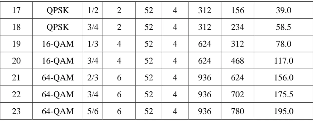
17 QPSK 1/2 2 52 4 312 156 39.0 18 QPSK 3/4 2 52 4 312 234 58.5 19 16-QAM 1/3 4 52 4 624 312 78.0 20 16-QAM 3/4 4 52 4 624 468 117.0 21 64-QAM 2/3 6 52 4 936 624 156.0 22 64-QAM 3/4 6 52 4 936 702 175.5 23 64-QAM 5/6 6 52 4 936 780 195.0

Table 05 rate dependent parameters for mandatory 20 MHz, Nss=4 (NES = 2) modes

MCA index Modulation R Nbpsc Nsd Nsp Ncpbs Ndbps Data rate (Mbps) 24 BPSK 1/2 1 52 4 208 104 26.0 25 QPSK 1/2 2 52 4 416 208 52.0 26 QPSK 3/4 2 52 4 416 312 78.0 27 16-QAM 1/3 4 52 4 832 416 104.0 28 16-QAM 3/4 4 52 4 832 624 156.0 29 64-QAM 2/3 6 52 4 1248 832 208.0 30 64-QAM 3/4 6 52 4 1248 936 234.0 31 64-QAM 5/6 6 52 4 1248 1040 260.0 R: Coding Rate

Nss: Number of Spatial Streams Nsd: Number of Data Subcarriers Nsp: Number of pilot subcarriers

Nbpsc: Number of coded bits per subcarrier per spatial stream

Ncbps: Number of Code Bits Per OFDM Symbol (total of all spatial streams) Ndbps: Number of data bits per MIMO-OFDM symbol

2.4 Transmitter Block Diagram

Figure 08 Transmitter diagram

The transmitter is composed of the following blocks:

z Scrambler – scrambles the data to prevent long sequences of zeros or ones – see section 4.2.

z Encoder Parser – de-multiplexes the scrambled bits among Nes FEC encoders, in a round robin manner.

z FEC encoders – encodes the data to enable error correction – an FEC encoder may include a binary convolutional encoder followed by a puncturing device, or an LDPC encoder.

z Stream Parser – divides the output of the encoders into blocks that will be sent to different interleaver and mapping devices. The sequences of the bits sent to the interleaver are called spatial streams.

z Interleaver – interleaves the bits of each spatial stream (changes order of bits) to prevent long sequences of noisy bits from entering the FEC decoder.

constellation points (complex numbers).

z Spatial Mapping – maps spatial streams to different transmit chains. This may include one of the following:

° Direct mapping – each sequence of constellation points is sent to a different transmit chain.

° Spatial expansion – each vector of constellation points from all the sequences is multiplied by a matrix to produce the input to the transmit chains.

° Space Time Block coding – constellation points from one spatial stream are spread into two spatial streams using a space time block code.

° Beam Forming - similar to spatial expansion: each vector of constellation points from all the sequences is multiplied by a matrix of steering vectors to produce the input to the transmit chains.

z Inverse Fast Fourier Transform – converts a block of constellation points to a time domain block.

z Cyclic shift insertion – inserts the cyclic shift into the time domain block. In the case that spatial expansion is applied that increases the number of

transmit chains, the cyclic shift may be applied in the frequency domain as part of spatial expansion.

z Guard interval insertion – inserts the guard interval.

z Optional windowing – smoothing the edges of each symbol to increase spectral decay

Parameter Value in legacy 20MHz channel Value in High Throughput 20MHz channel Value in High Throughput 40MHz channel NSD: Number of data subcarriers 48 52 108 NSP: Number of pilot subcarriers 4 4 6 NST: Total Number of subcarriers 52 56 114 NSR: Number of subcarriers occupying half of the overall BW 26 28 58 The spacing of subcarrier 312.5kHz (20MHz/64) 312.5kHz 312.5kHz (40MHz/128) TFFT: IFFT/FFT

period 3.2µsec 3.2µsec 3.2µsec TL-STF: Legacy

Short training sequence length

8µsec=10× TFFT/4 8µsec 8µsec

TL-LTF: Legacy Long training sequence length 8µsec=2× TFFT+TGI2 8µsec 8µsec TSYM: Symbol

Chapter 3

The Brief of Innovative Quixote DSP Board

3.1 About Quixote

Quixote is Innovative Integration’s Velocia-family baseboard. Velocia is an advanced architecture DSP baseboard that integrates a high performance Texas Instruments TMS320 C64xx DSP and Xilinx high density programmable logic with high performance peripherals such as PMC modules, analog IO and interconnectivity interfaces. The powerful combination of the DSP and FPGA provide signal processing speed and flexibility for almost any DSP application. Each baseboard features a PCI backbone connecting the DSP, PMC, peripherals and StarFabric interfaces. The StarFabric interface (PICMG 2.17) provides unlimited and extremely flexible interconnection to other DSP cards, IO cards and host processor systems. Each Velocia card incorporates a high performance IO system with either on-board peripherals like A/D and D/As, or one or more PMC sites accommodating a wide range of I/O options. Quixote DSP baseboard is for wireless, RADAR, ultrasound, high energy physics and other demanding applications requiring speed and processing power. Quixote features a powerful processing core built around Texas Instruments TMS320C6416 and Xilinx Virtex2 (2M or 8M gates) with 32MB of DSP RAM and 2MB of FPGA computation RAM (optional). Analog IO features include dual channels Quixote adds two (2) channels of 14-bit, 105 Mbps analog-to-digital (A/D) conversion and two (2)

channels of 14-bit, 105 Mbps digital-to-analog (DAC) conversion plus a 2 or 8 M user-programmable FPGA. The card serves a variety of applications including RF processing, radio-communications, servo applications, data acquisition and many others. System expansion is over StarFabric in a PICMG 2.17 compatible compact PCI chassis.

3.2 Support libraries

In order to support the baseboard as a part of a complete system, a complete set of powerful software libraries is provided to program the DSP on the baseboard and also to allow the card to interact with a host program resident on the PC. The Pismo Class Library provides support for developing applications which run on the target baseboard. The Armada Library provides the library support for host application development.

The Pismo Class Library

Pismo provides extensive C++ class support for： 1. Dynamic creation and runtime control of tasks

2. Simplified management of and access to all TI Chip Support Library (CSL) and DSP/BIOS API functions including: Semaphores, Mutexes, Mailboxes, Timers, Edma, Qdma, Atoms, McBsp, Timebases, Counters, etc.

3. Data exchange using RTDX Streaming I/O

4. Foundation (base) classes for DMA-driven device driver development 5. Templatized queues

The Armada Class Library

Armada is the Innovative Integration-authored component suite, which combines with the Borland BCB or Microsoft MSVC Integrated Development Environments (IDEs) to support programming of the Matador baseboard. Armada supports both high-speed data streaming plus asynchronous mailbox communications between the DSP and the Host PC, plus a wealth of Host functions to visualize and post-process data received from or to be sent to the target DSP.

The Armada suite shields the user from the nitty-gritty details of responding to asynchronous notifications of stream data and message reception, stream data requirements and message acknowledgements. Instead, a set of special C++ software class objects, called components, have been created to model each portion of the system. By employing software objects which model the true physical layout of the system, we can make a full-featured system more understandable.

The Caliente

Caliente is the internal, high performance data streaming support software within Armada. It is packaged both as an internal .component. for Borland VCL users and as a DLL for MSVC users. It handles bi-directional streaming of data between the host memory and the target DSP. The two streams are independent of each other, and may even be running at different rates.

When input streaming, the target DSP application and Host PC baseboard component must use identical channel configurations, in order for the channelization features of Caliente to function properly. The mechanism to create these configurations is described in a later chapter. When streaming starts, the baseboard collects data and busmasters it to the host memory. Caliente then moves the data into a set of internal buffers (called Pool Buffers), where the data is examined and split into individual data channels for use by the application. Caliente assumes that the data format that will be produced by the baseboard matches the configuration required by the pump components used within the Host application and can, therefore, properly separate the channels into independent streams and pump the data into the application for real-time processing.

Output streaming works similarly, but in the opposite direction. When data needs to be sent to a baseboard, Caliente requests sample data for the appropriate device channel from data pump components contained within Armada-based application software. When the data is received, the data is collated with data received from all other active channels, converted into peripheral-specific format and copied into bus-master memory. When the baseboard needs more data, it will automatically busmaster this data to its own onboard data storage, from which it sends the data to the appropriate output hardware.

Chapter 4

Developing A DSP Program

4.1 A recommended flow of developing a DSP program

Traditional development flows in the DSP industry have involved validating a C model for correctness on a host PC or Unix workstation and then painstakingly porting that C code to hand coded DSP assembly language. This is both time consuming and error prone. This process tends to encounter difficulties that can arise from maintaining the code over several projects.

The recommended code development flow involves utilizing the C6000 code generation tools to aid in optimization rather than forcing the programmer to code by hand in assembly. These advantages allow the compiler to do all the laborious work of instruction selection, parallelizing, pipelining, and register allocation. This allows the programmer the ability to focus on getting the product to market quickly. These features simplify the maintenance of the code, as everything resides in a C framework that is simple to maintain, support, and upgrade.

It is recommended that we follow the code develop flow below when we are writing and debugging our code.

Figure 09 A flow of developing a DSP program

4.2 Analyzing the C code performance

One of the preliminary measures of code is the time it takes the code to run. In large applications, it makes sense to optimize the most important sections of code first. Use the clock( ) and printf( ) functions in C/C++ to time and display the performance of specific code regions. The following example demonstrates how to include the clock() function in your C code.

Figure 10 A example to show the executing time

4.3 Refine the C/C++ code

4.3.1 Using the intrinsic to replace complicated C/C++ code

The C6000 compiler provides some intrinsic, special functions that map directly to inline C62x/C64x/C67x instructions to optimize your C/C++ code. All instructions that are not easily expressed in C/C++ code are supported as the intrinsic. The intrinsics are specified with a leading underscore ( _ ) and are accessed by calling them as you call a function. The following table shows some intrinsics.

Table 06 C compiler intrinsic

C Compiler Intrinsic Assembly Instruction Description

int _abs(int src2); ABS Return the saturated absolute value of src2

int _add4 (int src1, int src2); ADD4

Performs 2s-complement addition to pairs of packed 8-bit numbers.

unsigned _bitr (unsigned src); BITR Reverses the order of the bits

int _dotpn2 (int src1, int

src2); DOTPN2

The product of signed lower 16-bit values of src1 and src2 is subtracted from the product of signed upper 16-bit values of src1 and src2.

double _mpy2 (int src1, int

src2); MPY2

Returns the products of the lower and higher 16-bit values in src1 and src2.

4.3.2 Loop Unrolling

Another technique that improves performance is unrolling the loop; that is, expanding small loops so that each iteration of the loop appears in your code. This optimization increases the number of instructions available to execute in parallel.

4.3.2 Word access to the packed data

If we want to add 16-bit data vector, we can pack two 16-bit data into one 32-bit data. And then, do 32-bit addition with no carry at bit 16 which TMS320C64XX support. Like Using these word access to operate on 16-bit data stored in the high and low parts of a 32-bit register, we can save more time.

Figure 12 A example to show word access to packed data

4.3.2 Using compiler option

Compiler Options control the operation of the compiler. It can translate C code to assembly with attaching to debug capability, executing time or code size.

‹ -pm

Combines source files to perform program-level optimization by allowing visibility to the entire application.

‹ -o#

Optimizes register usage, locally or globally, file or program level.

‹ -ms#

Optimizes primarily for code size, and secondly for performance. Code size on three level (-ms0, -ms1, -ms2)

4.3 Write linear assembly code

If some function’s performance still does not achieve the requirement by refining C code using above methods, we can write assembly code by ourselves.TMS320C6x provides linear assembly language to user. It is no need to assign which register to use in one instruction comparing to original assembly language. Because it isn’t assigning register, parallel executing the instruction is also can not done by user appoint but by linear assembly optimizer.

A linear assembly file has a extended filename *.sa and it will be noticed that several points like:

1. Program label will start at the first character in one line.

2. Instruction can not start at the first character, it must follow the space.

3. There are some mnemonic which are machine – instruction or optimizer directive can help your program.

Table 07 some common linear assembler’s Directive

Directive Description Restrictions .call Calls a function Valid only within procedures .cproc Start a C/C++ callable

procedure Must use with .endproc .endproc End a C/C++ callable

procedure Must use with .cproc .mptr Avoid memory bank conflicts

Valid only within procedures; can use variables in the register parameter

.reg Declare variables Valid only within procedures .reserve Reserve register use Valid only within procedures

.return Return value to procedure Valid only within .cproc procedures

Here is a linear assembly code function which can be called by C function

Figure 13 A example to show a C callable function writing by linear assembly

Chapter 5

DSP Board Implementation Result and

Discussion

5.1 Choose M = 4 in SLM structure

802.11n is set up for wireless communication, it adopted MIMO OFDM structure, and choose FFT length 64. Because 64 is not too long so as we choose M = 4 in SLM structure is enough to deal with its PAPR problem. We can see fig 12 to know PAPR in the original OFDM structure will excess 9dB at the probability about 0.05, but applying to SLM with M=4, the probability is decrease to about 0.0001.

5.2 The use of the conversion matrix

Because choosing M = 4, we need to select additional three independent phase rotate vector. See chapter 1.2, using the conversion matrix can greatly lower the complexity of the original SLM structure. We select three phase rotate vector of the form [1, j , 1, j ] , [1, j , 1, -j ] and [1, j , -1, j ]. Figure 13 shows this conversion has no performance decade comparing to the IFFT banks. Table 8 shows the comparison of computation complexity between IFFT bank and conversion matrix.

5 6 7 8 9 10 11 12 13 10-5 10-4 10-3 10-2 10-1 100

probability of the PAPR exceeds the threshold for SLM with 64-pt FFT , L=4,

threshold P (PA PR > t h re s h o ld ) d B original

SLM with M = 4(using IFFT bank) SLM with M = 4(using conversion matrix)

Figure 15 The CCDF of PAPR comparison between IFFT bank and conversion matrix

Table 08 computation complexity between IFFT band and conversion matrix IFFT bank Conversion matrix respect to [1, j , 1, j ] Conversion matrix respect to [1, j , 1, -j ] Conversion matrix respect to [1, j , 1, -j ] Complex multiplication Nlog2N 0 0 0 Complex addition Nlog2N 6*N 6*N 6*N

5.3 About insert the side information

We still don’t consider side information up to now, and side information insertion usually means that bit rate will decrease. It is the expense which we choose SLM to lower the PAPR.

We should reserve several tones to transmit side information to the receiver side. It will need 2 (log2M) bit to indicate which phase rotate vector is been used when M=4.

In order to prevent the side information being corrupt by noise easily so as to make whole symbol is wrong, we need to apply channel coding to the side information bit and use low order modulation on the side information tones.

Fig14 simulate the PAPR of the 64-pt FFT length OFDM structure, SLM structure that information tones are reserved but not transmitting side information, and SLM structure with transmitting side information at the different power level on the information tones. The modulation type is BPSK to resist the noise. The side information is pass channel coding with (5, 2) shorten hamming code which can detect

two errors and correct one error.

Figure 16 SLM structure with transmitting the side information

5.3 Fixed point format on the DSP board

There are usually several restrict on the modulation accuracy in most spec, we should choose the fixed point format to fit this requirement. Due to not find the modulation accuracy requirement in 802.11n spec, we reference to 802.16 spec’s error vector magnitude (EVM.) It is obvious that 8-bit is not achieving requirement, so we choose 16-bit fixed point format to represent fraction number.

Table 09 simulation EVM result At the output of QAM

mapping

At the input of IFFT At the output of IFFT EVM(﹪) when using

8 bit to quantize 6.6 6.6 6.98

EVM(﹪) when using

16 bit to quantize 1.462* 10

-3

1.462* 10-3 5.854 * 10-2

5.3 Code performance on the DSP board

Table8 shows the comparison of PC and DSP bit rate and execute time. Fig14 shows the percentage of the block execute time in the simulation.

Table 10 execute time and bit rate At the PC At the DSP(without

optimized) At the DSP(with optimized) Execute time(s ) 3.578 3.0376 1.032 Bit rate(bit/s) 89435.43 105346.27 310077.59 execution time 7% 14% 4% 9% 6% 5% 7% 27% 6% 7% 8% info encode strmpasr freqintlv QAMmap STBC pilot IFFT SLM CS GI

Figure 17 the percentage of the all block execution time

5.4 About using the digital IO

Quixote provides 40 bits of bidirectional digital I/O. The digital I/O port allows the baseboard to exchange digital handshaking and information signals with other hardware, control and signal other devices, and may be used for software troubleshooting tasks as well. The user DIO (UD) port that has separate control and data registers that allows byte-wide control of the direction. The UD digital IO port is on connector JP5 (MDR50 connector). See the appendix for the connector pinouts.

1. About setting: make sure to include right DSP/BIOS configuration and the DIO is contained. ( Choosing the Quixtoe in the board category page or copy the existed project setting directly ).

2. Make sure to include UserData.h header.

The digital IO class

5.5 The estimate of speeding up the program using FPGA

Speeding up the program, it is needed that analyzing your application to identify the operations that are high speed (above 1 MHz) and lower speed. Higher speed signal processing operations should be targeted at the FPGA provided that they are of manageable complexity. Typical FPGA operations include FIR filters, down conversion, specialized high speed triggering and data sampling, and FFTs. All of these functions are deterministic mathematical functions that are suitable for the FPGA. Data formatting, protocols and control functions are typically more easily implemented on the DSP.

The Quixote has two FPGAs: a Xilnx Spartan2 (200K gates) and a Xilinx Virtex2 (2M or 6M gates). The Virtex2 is used for the analog interfacing, and as the computational logic on the board. Major elements inside the Spartan2 logic are the PCI interface, interrupt control, timebase selection and message mailboxes.

Quixote also provide some available clock. When we like developing the custom logic, we will need using the refclk which has about 20MHz frequency.

Block FFT:

The number of the stage is log2(N) in the N-point FFT structure. It can reach the

maximum data rate is 20M * N / log2(N) if FFT stages can be done in the 20MHz

clock period. Put the result in the 802.11n system (using 64-pt FFT), the maximum data rate is 20M * 64 / log2(64) = 213.33Mbit/s.

Block convolution encoder

There are six registers in the spec. 802.11n convolution encoder structure. Like the case in the FFT block, the maximum data rate depends on if we can put all logic into the 20MHz clock. We can reach the data rate about 20MHz when we really put into the 20MHz clock.

Table 11 speeding-up estimate using FPGA The estimated maximum

data rate by FPGA

data rate by DSP

IFFT 213.33Mbits/s 3.508Mbits/s Convolution encoder 40Mbits/s 0.55026Mbits/s

the estimate data rate using FPGA 0 50 100 150 200 250 FFT encoder func tion bl oc k

data rate (Mbits/s)

DSP FPGA

Chapter 6

Conclusion

SLM using conversion matrix is greatly lower the complexity comparing with the original IFFT bank in the original OFDM structure. Because MIMO-OFDM uses more transmit antenna, the complexity is needed lower in the every transmit antenna hardware dealing with the PAPR. In addition, 802.11n spec use 64 point FFT length, it is not too long as to very serious PAPR problem. So, we use SLM structure with conversion matrix but PTS structure in the 802.11n structure to reduce the PAPR. SLM has not bad performance but greatly lower complexity comparing with other PAPR reduction method. And insert the side information by low complexity way, we also add a power level parameter to trade off between the PAPR reduction capability and power on side information. This thesis also conclude something about how to use DSP board to develop a efficient program.

Chapter 7

Reference

[1] H. Ochiai and H. Imai, “Performance Analysis of Deliberately Clipped OFDM Signals,” IEEE Trans. on Commun., vol. 50, pp. 89–101, Jan. 2002.

[2] H. Saeedi, M. Sharif, and F. Marvasti, “Clipping noise cancellation in OFDM systems using oversampled signal reconstruction,” IEEE Comm. Lett., vol. 6, pp. 73–75, Feb. 2002.

[3] A. E. Jones, T. A. Wilkinson, and S. K. Barton, “Block coding scheme for reduction of peak to mean envelope power ration of multicarrier transmission schemes, ” Electron. Lett., vol. 30, no. 25, pp. 2098 – 2099, Dec. 1994.

J. A. Davis and J. Jedwab, “Peak-to-mean power control in OFDM, Golay complementary sequences, and Reed- Muller codes,” IEEE Trans. Inform. Theory,

vol. 45, no. 7, pp. 2397–2417, Nov. 1999.

[4] K. Yang and S. Chang, “Peak-to-Average Power Control in OFDM Using Standard Arrays of Linear Block Codes,” IEEE Commun. Lett., vol. 7, no. 4, pp. 174–176, Apr. 2003.

K. Patterson, “Generalized Reed-Muller codes and power control in OFDM modulation,” IEEE Trans. Inform. Theory, vol. 46, no. 1, pp. 104–120, Jan. 2000.

[5] D. Wulich and L. Goldfeld, “Reduction of peak factor in orthogonal multicarrier modulation by amplitude limiting and coding,” IEEE Trans. on Commun., vol. 47,

no. 1, pp. 18–21, Jan. 1999.

Ratio by Optimum Combination of Partial Transmit Sequences,” Elect. Lett., vol. 33, no. 5, Feb. 1997, pp. 368–69.

[7] A. D. S. Jayalath and C. Tellambura, “Adaptive PTS Approach for Reduction of Peak-to-Average Power Ratio of OFDM Signal,” Elect. Lett., vol. 36, no. 14,

July 2000, pp. 1226–28.

[8] R. W. Ba¨uml, R. F. H. Fischer and J. B. H¨uber, “Reducing the peak-toaverage power ratio of multicarrier modulation by selective mapping, ” Electron. Lett., vol. 32, no. 22, pp. 2056 –2 057, Oct. 1996.

[9] M. Breiling, S. H. M¨ uller – Weinfurtner and Johannes B. Huber, “SLM peak-power reduction without explicit side information, ” IEEE Commun. Lett.,

vol. 5, no. 6, JUNE 2001.

[10] EunJung CHANG, HoYeol KWON, and John M. CIOFFI, “PAR Reduction of Multicarrier Signals Using Injected Tone Constellation”, IEICE TRANS. COMMUN., VOL.E89–B, NO.10 OCTOBER 2006

[11] Krongold, B.S., Jones, D.L. An active-set approach for OFDM PAR reduction ,” via tone reservation”, IEEE Commun. Mag., vol. 28, pp. 5-14, May 1990.

[12] Naoto Ohkubo † and Tomoaki Ohtsuki, “A Peak to Average Power Ratio Reduction of Multicarrier CDMA Using Selected Mapping”Vehicular

Technology Conference, 2002. Proceedings. VTC 2002-Fall. 2002 IEEE 56th

[13] Chin-Liang Wang, Ming-Yen Hsu, Yuan Ouyang, “A low-complexity peak-to-average power ratio reduction technique for OFDM systems”, Global Telecommunications Conference, 2003. GLOBECOM '03. IEEE