行政院國家科學委員會補助專題研究計畫期中進度報告
※※※※※※※※※※※※※※※※※※※※※※※※※
※
基因調控網路之組合型重建 (1/3)
※
※※※※※※※※※※※※※※※※※※※※※※※※※
計畫類別:■個別型計畫
□整合型計畫
計畫編號:NSC 94-2213-E-009-143-
執行期間:94 年 8 月
1
日至
95 年 7 月 31 日
計畫主持人:胡毓志
共同主持人:
計畫參與人員:吳秉蔚,賴昀君,張巽昌
本成果報告包括以下應繳交之附件:
□赴國外出差或研習心得報告一份
□赴大陸地區出差或研習心得報告一份
■出席國際學術會議心得報告及發表之論文各一份
□國際合作研究計畫國外研究報告書一份
執行單位:交通大學 資訊工程系
中
華
民
國
95 年
4
月
27
日
行政院國家科學委員會專題研究計畫期中進度報告
國科會專題研究計畫成果報告撰寫格式說明
Preparation of NSC Project Reports
計畫編號:NSC 94-2213-E-009-143
執行期限:94 年 8 月 1 日至 95 年 7 月 31 日
主持人: 胡毓志 交通大學 資訊工程系
計畫參與人員:吳秉蔚,賴昀君,張巽昌 交大 資工系
一、中文摘要 在本計劃執行的第一年中,我們針對 多數已常被應用於基因網路重建研究之方 法做了詳細的探討,這其中包含布林網 路,貝氏網路,線性網路等。本年度的目 標在於評估各個方法的優劣,希望藉由各 系統的研究與探討,奠定我們新系統的基 礎,在透過仔細的分析評估之後,我們決 定採用多策略結合方式,整合轉錄子結合 區與基因表現資訊做為基因調節模組的預 測依據。 關鍵詞:專題計畫、報告格式、國科會 AbstractDuring the first year for this project, we investigated those approaches that have been widely applied to genetic network research,
including Boolean Networks, Bayesian
Networks, Linear Models and Non-linear Models, etc. The goal of our first-year project is to evaluate the pros and the cons of these various methods on which our network
reconstruction system can be based.
According to the evaluation, we have
concluded that our new approach will be built under a multi-strategy framework that combines motif binding sites and gene expression profiles.
Keywords: genetic networks, Boolean
networks, Bayesian networks, motif binding sites
二、緣由與目的
藉由分析大量的基因體實驗資料來瞭 解 所 有 基 因 (gene) 及 其 產 物 (gene product,如蛋白質, rRNA, tRNA 等)在種 種刺激下所產生的交互作用,是功能基因 體學 (functional genomics)重要目的之 一。為了達成此一目的,我們必須以系統 化的方式、全面性的角度對基因及其產物 進行分析,以建構出這些分子在細胞進行 各種活動、接受外在刺激時的交互關係, 亦即基因調控網路(genetic networks, or gene regulatory networks)。基因調控網 路的建立,可以幫助研究人員瞭解參與細 胞內各種生化反應的因素,讓製藥、醫學、 生化研究人員將實驗資源集中於重要的基 因上;也可以作為研究人員的虛擬實驗平 臺,由電腦來模擬他們所提出的假設。 準確地預測轉錄調控模組,才能重建 正確的轉錄調控網路。因此,我們的研究 目的就是提升轉錄控模組的預測能力,並 以此建構具參考價值的轉錄調控網路。 目前已有許多不同的方法被應用於基 因調控網路的重建,我們針對其優缺點做 了評估,希望藉由已知的方法中尋找靈感 以作為我們新系統的基礎。 三、結果與討論 我們特別針對一些常使用於基因調控 網路重建的方法做了比較: 布林網路是以邏輯關係來描述基因調 控網路。其核心假設為: (1) 每一基因的表現程度可以分為高(表 現)、低(不表現)兩種層次。 (2) 每一段基因的表現程度可以由其他基 因的表現程度以及外在條件所形成的 布林函式來決定。
這種表式法的優點是易於藉由邏輯關係解 釋基因間的交互作用,而缺點則是資料需 求量高。在一個 M 個節點的布林網路中, 我們需要 M 2 個觀察點來求得正確的布林 關係。Liang et al. 提出演算法試圖解決 此一問題(Liang et al. 1998),他們假設 每一個基因的基因表現至多由 k 個輸入所 決定,則解出 M 個節點的布林關係所需要 的資料量的估計值為 log( ) 2k M 。除了資料需 求量過高外,布林網路的假設與在實際狀 況 也 有 所 出 入 。 因 此 , Silvescu 等 人 (Silvescu et al. 2001)及 Soinov 等人 (Soinov et al. 2001)都以 Decision Tree 來建立布林網路,並且試圖修正一般的布 林網路所忽略的時間因素。此外,Ilya Shmulevich 等人則為為布林網路加入機率 模式,來模擬細胞中生化反應的不確定性 (Shmulevich et al. 2002)。 線性模式是研究許多物理現象常用的 數學模式,而以線性模式來表示基因調控 網路的假設如下: (1) 每一段基因的表現程度是連續的,而 非離散狀態。 (2) 每一段基因的表現程度可以由其他基 因的表現程度以及外在條件以線性方 程式表達。 這種表示法優於布林網路的地方在於 保留了基因表現的原始資訊,但缺點則是 此方法並不如布林網路般易於解釋基因之 間的交互作用。在一個 M 變數的線性模式 中,所需的資料量為 M 個觀察點,但在目 前的應用中,我們仍沒有那麼多的生物實 驗 資 料 對 整 個 基 因 組 求 解 。 因 此 , D’haeseleer P.等人以內插法方式來增加 資 料 數 目 (D’haeseleer P. et al. 1999b);而 van Someren E. P.等人則利用 分群法將基因表現相似者視為同一個節 點,以減少整個基因調控網路的複雜度 (van Someren E. P. et al. 2000)。
貝 氏 網 路 (Bayesia Networks) 是 graphical models 之一,它以條件機率來 表示基因調控網路中各基因間的相關性。 其核心假設為: (1)每 一 個 節 點 可 代 表 可 觀 察 變 數 (information variables),如基因表 現 ; 或 者 是 不 可 觀 察 變 數 (latent variables),如外在刺激、蛋白質表 現、蛋白質結構、實驗誤差等。變數可 以是連續或離散狀態。 (2)變數間的關係分為相關(dependency) 以 及 條 件 獨 立 (conditional independence)。 (3) 給定資料 D 與假設的網路結構 S,若 S 的 事 後 機 率 (posterior probability)p(S|D)越大,代表在以資料 D 為證據下,網路結構 S 成立的機率越大。 貝氏網路的優點在於其模式能夠包含 不可觀察變數,並以事後機率來衡量可能 的網路結構,這些都有助於模擬真實世界 中的不確定性與變異性。其缺點是貝氏網 路必須先提出可能的網路結構,才能以實 驗資料來評估該結構的事後機率。而 M 個 結點的網路,有 M 2 種可能的結構,因此計 算出 global optimal solution 所需計算 量 過 大 , 其 時 間 複 雜 度 為 NP-complete(Fisher et al. 1996) 。 Hartemink 等人則利用 AI 中常見的幾種 heuristic search 方 法 來 找 出 local
optimal solution(Hartemink et al.
2002)。 根據以上的結論,我們決定採行整合 型的系統以重建基因網路,整合多種資 訊,包含轉錄調控區間、基因表現實驗, 以及已知的轉錄因子結合區,其目的是預 測被這些轉錄因子所調控的基因,也就是 轉錄調控模組,並將預測的轉錄調控模組 整合成轉錄調控網路。而預測轉錄調控模 組的核心假設為: (1)在其轉錄調控區間含有特定轉錄因子 結合區的基因,可能會受到該轉錄因子 的調控。 (2)基因產物的行為,大部份決定於基因表 現程度。因此,產生轉錄因子所需的基 因,其基因表現程度與轉錄因子的行為 相關。 (3)轉錄因子所調控的基因,其基因表現程 度會受轉錄因子影響;間接的,也會與 構成轉錄因子的基因之表現程度相關。 Fujibuchi 等 人 曾 經 以 酵 母 菌 (Saccharomyces cerevisiae) 為 研 究 對 象,整合酵母菌基因組的轉錄調控區序 列、基因表現實驗、轉錄因子結合區等資
訊,定義出新的評分方式來對調控關係進 行篩選(Fujibuchi W. et al. 2001),其 研究結果顯示在整合了多種資訊後,可以 更準確地預測轉錄調控模組。Fujibuchi 等人的核心假設是受到共同轉錄因子所調 控的基因,其表現行為相似。由於我們的 假設與其有所不同,我們也將整合兩方的 評方分式,希望以更完整假設來預測轉錄 調控模組。 我們的整合型系統之重點在於結合 motif binding sites 與 expression profiles 的資訊,如此可加強基因調控模 組的預測準確性,此外,即便在 motif binding sites 資訊欠缺的情況下,亦可 藉由 expression profiles 的資訊找到逼 近的較佳解,這樣便可提升我們系統的實 用性。 為求將來實驗比較的統一性,我們已 蒐集了與 Fujibuchi 等人的研究相同的實 驗資料,其為 121 組在酵母菌上的基因表 現實驗所得,此外,我們也依循 Spellman 等人做了資料的前置處理,我們計畫於第 二年實做系統,並設計評估實驗。實驗目 的將包含基因調控模組的預測準確性評 估 , 以 及 利 用 已 知 的 基 因 網 路 作 為 benchmark 檢測系統的網路重建能力。 四、參考文獻
Cho R. J., Campbell M. J., Winzerler E. A., Steinmetz L., Conway A., Wodicka L., Wolfsberg T. G., Gabielian A. E., Landsman D., Lockhart D. J.,
and Davis R. W. (1998). A
Genome-Wide Transcriptional
Analysis of The Mitotic Cell Cycle. Molecular Cell, 2(1): 65-73.
Chu S., DeRisi J., Eisen M., Mulholland J., Botstein D., Brown P. O., and
Herskowitz I. (1998). The
Transcriptional Program of
Sporulation in Budding Yeast.
Science, 282(5389): 699-705.
DeRisi J. L., Iyer V. R., and Brown P. O.
(1997). Exploring the Metabolic
and Genetic Control of Gene
Expression on A Genomic Scale. Science, 278(5338): 680-686. D'haeseleer P., Wen X., Fuhrman S., and
Somogyi R. (1997). Mining the Gene Expression Matrix: Inferring
Gene Relationships from Large
Scale Gene Expression Data. In:
M.Holcombe, R.Paton(eds)
Information Processing in Cells and Tissues. Plenum, 203-212.
D'haeseleer P., Liang S., and Somogyi R. (1999a). Gene Expression Analysis and Genetic Network Modeling.
Pacific Symposium on
Bioinformatics, Tutorial session on
Gene Expression and Genetic
Networks.
D'haeseleer P., Wen X., Fuhrman S., and
Somogyi R. (1999b). Linear
Modeling of mRNA Expression Levels during CNS Development and Injury. Pacific Symposium on Bioinformatics, 4: 41-52.
Eisen M. B., Spellman P. T., Brown P. O., and Bostein D. (1998). Cluster
Analysis and Display of
Genome-Wide Expression Patterns. Proceedings of National Academy of Sciences, 95(25): 14863-14868.
Fujibuchi W., Anderson J. S., and
Landsman D. (2001). PROSPECT
Improves Cis-Acting Regulatory
Element Prediction by Integrating
Expression Profile Data with
Consensus Pattern Searches.
Nucleic Acids Res., 29(19):
3988-3996.
Hartemink A. J., Gifford D. K., Jaakkola T. S., and Young R. A. (2001). Using Graphical Models and Genomic
Expression Data to Statistically
Validate Models of Genetic
Regulatory Networks. Pacific
Symposium on Bioinformatics, 6: 422-433.
Hartemink A. J., Gifford D. K., Jaakkola T.
Combining Location and
Expression Data for Principled
Discovery of Genetic Regulatory Networks. Pacific Symposium on Bioinformatics, 6: 437-449.
Hertz, G. Z., Hartzell G. W. 3rd, and
Stormo G. D. (1990).
Identification of Consensus Patterns
in Unaligned DNA Sequences
Known to Be Functionally Related.
Computer Applications in the
Biosciences (now Bioinformatics), 6(2): 81-92.
Lashkari D. A., DeRisi J. L., McCusker J. H., Namath A. F., Gentile C., Hwang S. Y., Brown P. O., and Davis R. W.
(1997). Yeast Microarrays for
Genome Wide Parallel Genetic and Gene Expression Analysis. Proc. Natl. Acad. Sci. USA, 94(24): 13057-13062.
Lee T. I., Rinaldi N. J., Robert F., Qdom D. T., Bar-J. Z., Gerber G. K., Hannett N. M., Harbison C. T., Thompson C. M., Simon I., Zeitlinger J., Jennings E. G., Murray H. L., Gordon D. B., Ren B., Wyrick J. J., Tagne J.-B., Volkert T. L., Fraenkel E., Gifford K. D., and Richard A. (2002).
Transcriptional Regulatory
Networks in Saccharomyces
cerevisiae. Science, 298(5594):
799-804.
Liang S., Fuhrman S., and Somogyi R. (1998). Reveal, A General Reverse
Engineering Algorithm for
Inference of Genetic Network
Architectures. Pacific Symposium on Bioinformatics, 3: 18-29.
Mendenhall M. D., and Hodge A. E. (1998).
Regulation of Cdc28
Cyclin-Dependent Protin Kinase
Activity during the Cell Cycle of the Yeast Saccharomyces cerevisiae. Microbiol. Mol. Biol. Rev. 62(4): 1191-1243.
Shmulevich I., Dougherty E. R., Kim S., and
Zhang W. (2002). Probabilistic
Boolean Networks: A Rule-based
Uncertainty Model for Gene
Regulatory Networks.
Bioinformatics, 18(2): 261-274
Silvescu A., and Honavar V. (2001).
Temporal Boolean Network Models of Genetic Networks and Their Inference from Gene Expression Time Series. Complex Systems., 13(1): 54-.
Simon I., Barnett J., Hannett N., Harbison C. T., Rinaldi N. J., Volkert T. L., Wyrick J. J., Zeitlinger J., Gifford D. K., Jaakkola T. S., and Young R. A.
(2001). Serial Regulation of
Transcriptional Regulators in the Yeast Cell Cycle. Cell 106(6): 697-708.
Soinov L. A., Krestyaninova M. A., and
Brazma A. (2003). Towards
Reconstruction of Gene Networks
from Expression Data by
Supervised Learning. Genome
Biology, 4(1): R6.
Spellman P. T., Sherlock G., Zhang M. Q., Iyver V.R., Anders K., Eisen M. B., Brown P. O., Bostein D., and Futcher B. (1998). Comprehensive
Identification of Cell
Cycle-Regulated Genes of the Yeast
Saccharomyces Cerevisiae by
Microarray Hybridization.
Molecular Biology of the Cell, 9(12): 3273-3297.
Tamayo P., Slonim D., Mesirov J., Zhu O. Kitareewan S., Dmitrovsky E., and Golub T. R. (1999). Interpreting Patterns of Gene Expression with
Self-Organizing Maps: Methods
and Application to Hematopoietic Differentiation. Proc. Natl. Acad. Sci. USA, 96:2907-2912.
Tavazoie S., Hughes J. D. Campbell M. J., Cho R. J., and Church G. M. (1999).
Systematic Determination of
Nature Genet., 22:281-285.
van Someren E. P., Wessels L. F. A. and Reinders M. J. T. (2000). Linear
Modeling of Genetic Networks
from Experimental Data. Intelligent Systems for Molecular Biology, 8: 355-366.
行政院國家科學委員會補助國內專家學者出席國際學術會議報告
95 年 4 月 27 日報告人姓
名
胡
毓
志
服務
機構
及職稱
交通大學資訊科學系
副教授
時間
會議
地點
06/26/2006-06/29/2006 Las Vegas, USA本會核定
補助文號
NSC
94-2213-E-009-143-會議
名稱
(中文) 生物資訊暨計算生物學國際研討會
(英文)2006 International Conference on Bioinformatics and
Computational Biology
發表
論文
題目
1.(中文) 以多策略方法設計蛋白質結構字元
(英文)
A Multi-Strategy Approach to Protein Structural Alphabet Design因期中進度報告繳交期限在研討會舉行之前,因此,僅附上會議論文,請 參考。
附
件
A Multi-strategy Approach to Protein Structural Alphabet Design
Shih-Yen Ku and Yuh-Jyh Hu Department of Computer Science
National Chiao Tung University {gis92622,yhu}@cis.nctu.edu.tw
Abstract
The search for structural similarity among proteins can provide valuable insights into their functional mechanisms and their functional relationships. Though the protein 1D sequence contains the information of protein folding, the performance of predicting the 3D-structure directly from the sequence is still limited. As the increase of available protein structures, we can now conduct more precise and thorough studies of protein structures. Among many is the design of protein structural alphabet that can characterize protein local structures. We use the self-organizing map combined with the minimum spanning tree algorithm for visualization to determine the alphabet size and then apply the k-means algorithm to group protein fragments into clusters corresponding to the structural alphabet. The intra-cluster and inter-cluster analyses show the significant structural cohesiveness. A comparative study of our alphabet with one of the
recently developed structural alphabets also
demonstrated a competitive result.
1. Introduction
Various genome sequencing projects have been producing numerous linear amino acid sequences; however, complete understanding of the biological roles played by these
proteins requires knowledge of their
structures and functions [1]. Despite that experimental structure determination methods
provide reasonable structure information
regarding subsets of proteins, computational methods are still required to provide valuable information for a large fraction of proteins whose statures may not be experimentally
determined. Even though the primary
sequence implies the whole information
guiding the protein folding, yet the
performance of predicting the 3D-structure directly from the sequence is still limited. The
complexity and the number of
physicochemical, kinetic and dynamic
parameters involved in protein folding
prohibit an efficient 3D-structure prediction without first knowing the 3D-structures of closely related proteins [2]. Some ab initio methods do not directly use 3D-structures, but their applications are often limited to small proteins [3].
Early analysis of protein structures has shown the importance of repetitive secondary
structures, i.e. -helix and -sheet. With
variable coils, they constituted a basic
standard 3-letter alphabet, and this has led to
early secondary structure prediction
algorithms, e.g. GOR [4], and more recent
ones that apply neural networks and
homology sequences [5-8] with prediction accuracy approaching 80%. In spite of the
increase of predictive accuracy, the
approximation of 3D-structures with only a 3-letter alphabet is apparently too crude for
meaningful 3D reconstruction. All the
predictions are highly dependent on the
definitions of periodic structures, but
unfortunately the structure description is incomplete. As the increase of available protein structures, it allows more precise and
thorough studies of protein structures.
Various more complex structural alphabets have been developed by taking into account
the heterogeneity of backbone protein
structures through sets of small protein fragments frequently observed in different
protein structure databases [2][9]. The alphabet size can vary from several to around 100. For example, Unger et al. [10] and Schuchhardt et al. [11] used k-means method and self-organizing maps respectively to identify the most common folds, but the large number of clusters (about 100) is not appropriate for prediction. Rooman et al. found 16 recurrent folding motifs, ranging from 4 to 7 residues and categorized into four
classes corresponding to -helix, -strand,
turn and coil [12]. By applying
autoassociative neural networks, Fetrow et al.
defined six clusters representing
supersecondary structures that subsume the classic secondary structures [13]. Bystroff and
Baker produced similar short folds of
different lengths and grouped them into 13 clusters for prediction [14]. Taking into
account the Markovian dependence,
Camproux et al. developed an HMM
approach to lean the geometry of the
structural alphabet letters and the local rules for assembly process [15].
In this paper, we propose a multi-strategy approach to identifying structural alphabet that can characterize protein local structures. Instead of applying cross-validation [14] or shrinking procedures [16] to refine the clusters directly, we use self-organizing maps as a visualization tool to determine the size of structural alphabet. Given the alphabet size, we later apply the k-means algorithm [17] to group protein fragments into clusters that correspond to a structural alphabet. The analysis of structural similarities between proteins not only provides significant insight into functional mechanisms and biological relationships, but also offers the basis for protein fold classification. An expressive structural alphabet can allow us to quantify the similarities among proteins encoded in appropriate letters. It also enables us to work with a primary representation of 3D structures,
simply using standard 1D amino acid
sequence alignment methods. To demonstrate the performance of our new method, we tested it on the all-proteins in SCOP. The experimental results show that using our structural alphabet rather than the standard amino acid letters can outperform BLAST in finding the best hit for a protein query. This suggests that our structural alphabet can
successfully reflect protein structural
characteristics which are implied in protein fragments. Besides, in order to make a consistent and fair comparison, we also compared our alphabet with others that are also developed by the SOM, but in a different design methodology [9][19]. Our structural alphabet shows competitive performance in protein matching.
2. Material and methods
The use of frequent local structural motifs
embedded in polypeptide backbone has
recently shown improvement in protein
structure prediction [1][14][18]. Its success has shed some light on further studies of structural alphabet. We used the proteins classified to all- fold within the SCOP database (version 1.65) in our study with the aim to build the structural alphabet suitable for all-proteins. The same approach can be easily applied to other databanks as well.
There are three issues addressed in our
study. They are: (1) protein fragment
representation, (2) alphabet size
determination and (3) structural alphabet definition. Like others, we transform each protein backbone into a series of the dihedral angles ( and , neglecting ) [14][16]. Adapted from [16], the analysis is limited to fragments of five residues since they are
adequate for describing a short helix and a
minimal structure. With the fixed window
along each all-protein in SCOP, advancing one position in the sequence for each fragment, and collected a set of overlapped 5-residue fragments. As the relation between two successive carbons,
i C and 1 i C ,
located at the ith and (i+1)th positions, can be
defined by the dihedral angles i of Ci and
i+1 of Ci1, a fragment of L residues can
then be defined as a vector of 2(L-1) elements. Thus, in our study, each protein fragment,
associated with -carbons
2 i C , 1 i C , i C, 1 i C and 2 i C , is represented by a vector of
eight dihedral angles, i.e.
]. , , , , , , , [i2 i1i1 i i i1i1 i2 Based on
this representation, we totally gathered
1,143,072 fragment vectors.
Self-organizing maps (SOM) are widely used as a data mining and visualization tool for complex data sets. A self-organizing map usually consists of a regular 2D grid of so-called map units, each of which is
described by a reference vector mi= [mi1, mi2,
mi3,…, mid], where d is the input vector
dimension, e.g., d = 8, in our case of fragment vectors. The map units are usually arranged in a rectangular or hexagonal configuration. The number of units affects the generalization capabilities of the SOM, and thus is often specified by the researcher/user. It can vary from a few dozen to several thousands. An SOM is a mapping from the ensemble of
input data vectors (Xi=[xi1, xi2, xi3,…, xid]Rd)
to a 2D array of map units. During training, data points near each other in input space are mapped onto nearby map units to preserve the topology of the input space [19][20]. The SOM is trained iteratively. In each training step t, distances between a randomly picked
input vector xj and all the reference vectors
are computed. The unit with the least distance is then selected as the winner unit and denoted by w. The winner unit and its
topological neighbors are updated to move
closer to input vector xj in the input space by
the following rule:
) ( ) ( ) ( ) ( ) 1 (t m t t h t x m t mi i wi j i
where t is time, (t) is the adaptation
coefficient, |xj-mi(t)| is the component-wise
difference between the input vector and the
ith reference vector, and hwi(t) is the
neighborhood function acting on the array of units, whose form includes bubble kernel, Gaussian kernel and other more complicated ones. In our study, we used the bubble kernel [20][21]. Unlike previous works that directly apply SOM to obtain clusters of backbone fragments as the basis to define the structural alphabet, our approach instead uses SOM
only for the visualization purpose to
predetermine the number of letters in the alphabet.
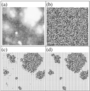
By visual inspection of the trained SOM, we can get a preliminary idea of the number of clusters on the map. The unified distance matrix (U-matrix) is one of the most widely used methods for visualizing the clustering result on the SOM. It shows distances between neighboring reference vectors, and can be efficiently visualized using grey shade [22], as shown in Figure 1(a). In spite of the initial idea of the cluster structure provided by
the U-matrix, a systematic method to
determine the number of clusters on the map is still desired. We implement a post-process on the U-matrix that is based on the minimum-spanning-tree algorithm. Given the grey levels in the U-matrix, we can build the minimum spanning tree for all the map units, e.g., in Figure 1(b), all map unit are linked in the spanning tree. Based on a threshold of the grey level, we can partition the entire tree into several disconnected subtrees, by removing the links between map units with grey levels below the threshold, as shown in Figure 1(c). Conceptually, it means that we break the links of a distance longer than some threshold.
Furthermore, those relatively smaller subtrees left can be also deleted later such that the remaining clusters can maintain a reasonable size, as presented in Figure 1(d). The number of the subtrees finally kept becomes the structural alphabet size. As the SOM can be viewed as a topology preserving mapping from input space onto the 2D grid of map units [19], the number of map units can affect
the clustering result. We systematically
increase the number of units, and repeat the above process till the alphabet size stabilizes.
Rather than adapt the two-level approach that first trains the SOM, then performs clustering of the trained SOM [19], after determining the alphabet size, we apply the k-means algorithm to the input data vectors directly to obtain the clusters. The SOM established a local order among the set of reference vectors in such a way that the closeness between two reference vectors in
the Rd space is dependent on how close the
corresponding map units are in the 2D array. Nevertheless, an inductive bias of this kind
may not be appropriate for structural
alphabets since the local order does not always faithfully characterize the relation between structural building blocks, and can sometimes be misleading, e.g. forcing the topology to preserve mapping from the input
space of-helix and -strand to a 2D grid of
units could be harmful to clustering. As a result, we use the SOM only for visualization the alphabet size, and rely on the k-mean algorithm to extract the local features from the input data that can actually reflect the characteristics of the clusters respectively. The centroid of each cluster forms the prototypical representation of each alphabet letter. Given the clustering result by the k-means algorithm as the basis of the structural alphabet, we can transform a protein into a series of the alphabet letters by matching each of its fragments against our
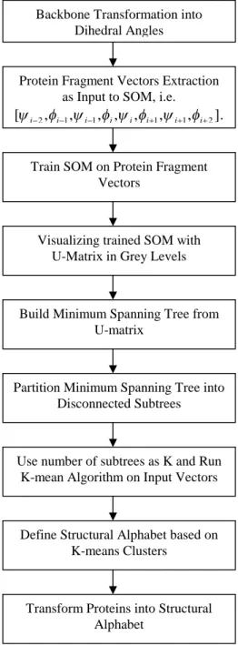
alphabet prototypes. The control flow of our system named SMK is illustrated in Figure 2.
(a) (b)
(c) (d)
Figure 1. Visualization of the trained SOM. (a) the grey shade of the trained SOM, where darker areas mean larger distances, (b) the minimum spanning tree for the map units, (c) the disconnected subtrees after removing the links below some threshold and (d) the final disconnected subtrees after discarding those relatively small ones.
3. Experimental results
We tested our approach on the all- proteins in SCOP. By this experiment, we show that our method can produce an appropriate structural alphabet for describing
these all- proteins. After transforming
protein backbones into dihedral angles and extracting protein fragments, we trained the SOM on these dihedral angle vectors.
Three issues were addressed in the
experiments. First, the meaningfulness of the structural alphabet size in terms of the number of clusters was presented by showing the size stability given various parameters.
cohesiveness by visual superimpositions of protein fragments as well as computed the intra-cluster and inter-cluster distance. Third, we proved the fragment clusters found were not arbitrary by comparing our result with that from a random background.
Figure 2. The system control flow of SMK
Since the number of map units has
influence over the SOM’s clustering behavior,
to obtain the optimal number of clusters, we varied the number of units on the map until the number of clusters found became steady. The results are shown in Figure 3, which indicates a distinctive plateau within the range between nine and twelve. Because eleven is the most frequent number of clusters on the plateau, as shown in Figure 4, it is designated as the structural alphabet size.
To further confirm the general geometric regularities characterized by the structural alphabet, we also built a negative all- protein fragment set for comparison. The negative set was derived from the real all- protein fragment vectors prepared earlier by
rotating the dihedral angles at random
(increase or decrease) within a certain degree, e.g. 30in our analysis. We compared the clusters produced by clustering on the real vector set and on the negative control set. Insignificant difference suggests that the alphabet we found could be arbitrary. Our
experiments (see Figure 5) show that
clustering on the negative control set cannot
even produce consistent clusters, which
supports our hypothesis that the clusters found from the real fragment vectors reflect
the classes of local protein structures;
otherwise, these clustering results would have been similar.
Given the size, we ran the k-means algorithm on the input fragment vectors to find the twelve clusters by which to define the structural alphabet. Figure 6(a) and (b) shows
the fragment superimpositions for the
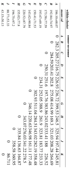
alphabet. Even though the fragment structures do not superimpose perfectly, yet the general structural cohesiveness of each category is quite evident. In addition, we computed the Euclidean distances from each fragment in a given cluster to its centroid. The average of
these within-cluster distances was then
Backbone Transformation into Dihedral Angles
Protein Fragment Vectors Extraction as Input to SOM, i.e.
]. , , , , , , , [i2 i1i1 ii i1i1i2
Train SOM on Protein Fragment Vectors
Visualizing trained SOM with U-Matrix in Grey Levels
Build Minimum Spanning Tree from U-matrix
Partition Minimum Spanning Tree into Disconnected Subtrees
Use number of subtrees as K and Run K-mean Algorithm on Input Vectors
Define Structural Alphabet based on K-means Clusters
Transform Proteins into Structural Alphabet
compared with the center-to-center distances between clusters as presented in Table 1. It shows that in most cases, the center-to-center distance between any two clusters is greater than the mean distance of all vectors in that cluster from its center plus one standard
deviation. The result indicates that the
individual clusters are fairly well separated from each other.
The detection and analysis of structural similarities between proteins allows deeper insight into their functional mechanisms and
relationships. To search for structural
similarities, the structural alphabet provides a good basis on which to work with a 1D representation. As a result, numerous 1D alignment algorithms can be used, with minor modifications, to detect structural similarities. In our experiments, we first transformed the 3D structures of proteins into a 1D sequence of the letters in our structural alphabet. To demonstrate the applicability of the alphabet, we used FASTA to search for structural similarities between a query protein and a
bank of proteins, using an
identify matrix of our
0 10 20 10X1 0 60X6 0 110X 110 160X 160 210X 210 map size nu m be r of cl us te r
Figure 3. The variance in the number of
clusters produced by the SOMs of varying sizes. There exists a distinctive plateau that suggests the cluster number has stabilized.
0 2 4 6 8 1 6 11 16 21 number of cluster fr en qu en cy
Figure 4. The frequencies of cluster numbers. It shows 11 is the most frequent number of clusters. 0 10000 20000 30000 40000 10X1 0 60X6 0 110X 110 160X 160 map size nu m be r of cl us te r
Figure 5. The variance in the number of clusters produced by the SOMs of varying sizes trained on a negative fragment set. It shows no sign of convergent cluster number.
alphabet letters to find maximal exact
matches. For comparison, we also conducted the same tests also using FASTA but based on different structural alphabets, one developed by de Brevern et al. [9], the other by the
two-level SOM approach [19]. As the
baseline reference, we used BLAST with the standard 20 amino acid letters to find the best sequence hit.
The proteins used in the experiments were selected from the all- proteins in SCOP. After filtering out those with more than 30% sequence similarity, we have totally 1055 proteins. For each run of the experiment, we randomly picked one protein as the query, and then matched it against the rest, using FASTA or BLAST with different alphabets. Given the
best hit, we computed the RMSD
between the query and the hit,
Table 1. Summary of within-cluster distances and center-to-center distances. K J I H G F E D C B A 4 3 .1 5 ± 5 0 .1 3 8 8 .7 7 ± 5 3 .3 3 1 9 6 .7 5 ± 9 7 .2 1 5 5 .0 2 ± 7 7 .8 2 2 0 .5 2 ± 8 7 .7 9 1 4 3 .6 2 ± 9 0 .8 4 1 5 0 .4 1 ± 7 1 .5 3 1 9 3 .6 7 ± 6 9 .1 9 1 7 3 .5 8 ± 7 7 .5 9 1 9 2 .8 4 ± 7 4 .9 7 1 8 6 .1 0 ± 6 8 .0 7 m ea n ± sd w it h in -c lu st er 0 A 0 2 8 2 .3 B 0 2 8 4 .5 9 2 0 5 .2 7 C 0 2 5 0 .3 1 2 0 3 .4 1 2 1 6 .7 5 D 0 2 3 4 .3 1 2 5 1 .6 2 0 2 .8 2 2 6 .9 3 E 0 3 0 2 .9 3 2 5 2 .0 5 1 9 7 .7 6 2 7 5 .0 8 2 3 6 .7 2 F 0 3 4 6 .1 4 5 1 1 .0 4 3 8 8 .9 3 8 3 .8 6 4 1 4 .9 9 3 9 9 .5 3 G 0 3 4 3 .0 7 2 2 0 .6 3 2 8 4 .5 1 2 6 1 .9 2 4 3 .0 2 1 6 9 .3 2 4 6 .5 H 0 3 3 5 .8 4 2 7 6 .0 3 3 4 6 .9 8 3 4 3 .0 2 3 2 3 .8 1 3 3 3 .4 1 3 2 1 .0 3 3 2 5 .9 4 I 0 3 5 8 .5 8 1 3 6 .6 3 3 4 1 .2 2 1 6 1 .1 1 2 8 2 .1 9 1 8 3 .7 7 1 8 8 2 0 8 .2 8 1 9 7 .4 4 J 0 8 6 .7 1 1 3 6 0 .9 5 1 6 4 .8 7 2 7 8 .5 1 7 7 .4 8 3 5 8 .4 8 2 3 3 .3 3 2 2 6 .5 2 2 6 4 .6 9 2 4 5 .8 1 K ce n te r-to -c en te r
and recorded the lowest level in the SCOP hierarchy at which the query and the hit are both located, i.e. class, fold, superfamily or family. Smaller RMSD and lower common level in SCOP hierarchy indicates higher
structural similarity. We repeated the same experiment for 100 times and the results are summarized in Table 2 and 3. According to Table 2, we notice that our method SMK and
de Brevern et al.’s both produced higher
frequencies at lower common levels than the other two methods. This suggests that our
structural alphabet and de Brevern et al.’s can
better characterize the SCOP hierarchy. Table 3 shows that SMK has the lowest mean RMSD and standard deviation among all.
Table 2. Summary of frequencies at the lowest common level. The first column shows the methods used in the experiments. The remaining columns present the frequency for different levels at which the query and the best hit are both located.
frequency at different level
Method class fold super family family
BLAST 71 4 5 20
SMK 55 11 5 29
de Brevern 58 4 11 27
2-level SOM 73 6 14 7
Table 3. Summary of average RMSD and standard deviation between the queries and the best hits.
method mean (RMSD) sd (RMSD) BLAST 8.953744 4.764597 SMK 7.290972 3.934283 de Brevern 8.076746 4.819178 2-level SOM 10.38624 5.217078
4. Discussion
In this paper, we propose a multi-strategy approach to designing the structural alphabet which allows local approximation of protein
3D structures as well as enables the applications of 1D alignment algorithms to search for 3D structural similarities. The success of the alphabet design depends on three crucial factors. First, it is the protein fragment representation, which determines what and how 3D structural characteristics to
be approximated, e.g. thermodynamic
stability, amino acid physicochemical
properties, amino acid usage in known
proteins, distances, dihedral angles, bond lengths, bond angles, etc.
A B C D E F G H I J K
Figure 6(a). The superimposition in
wireframe format for the structures of each structural cluster found by SMK.
A B C D E F G H I J K
Figure 6(b). The superimposition of the structures of each structural cluster found by SMK in the ball-and-stick form.
The effects of the representation selected are
entangled with the performance of the
learning approach we apply to develop the
structural alphabet. Overcomplicated
representations can sometimes lead to
overfitting. To avoid this problem, we
currently focus on the dihedral angles. Other features can be easily included in the representation if proved necessary.
The second factor is the size of the alphabet. We took advantage of the SOM as a visualization tool that helps determine the alphabet size. By systematically varying the number of map units on the map, we visualized the clustering behavior of the SOM. Our experiments showed a distinct plateau corresponding to the convergent number of
clusters, compared with the increasing
number of clusters in the results of clustering on the random negative control dataset. This suggests that the structural alphabet size we found is not arbitrary.
Various types of algorithms have been
applied to clustering local protein 3D
fragments into a limited set of fold patters, e.g. self-organizing maps (SOM), hidden Markov models (HMM), neural networks, hierarchical clustering, k-means clustering, etc. Each has its own learning bias and inherent limitations. For example, the topology (e.g. number of layers or map units) of neural networks, the SOM and the HMM strongly affect the performance. The value of k in k-means algorithm determines the clusters. As a consequence, the third factor is the learning
algorithm. In our study, we took a
multi-strategy approach. We first used the
SOM and the minimum-spanning tree
algorithm to determine the alphabet size, and then applied the k-means algorithm to group
fragments into meaningful clusters. The
number of map units in the SOM and the value of k in k-means are not pre-specified in
advance, but instead determined
systematically. To verify the correspondence of our structural alphabet letter to the fold
patterns, we computed the average
within-cluster distance for each alphabet cluster as well as the distance across clusters. The small average within-cluster distance and the relatively large between-cluster distance demonstrate the significance of the structural
alphabet we found. Furthermore, the
visualized superimposition of protein
fragments in each cluster also justifies the structural cohesiveness.
The objective of the paper is to propose a new approach to developing the structural alphabet. To verify its usefulness, we tested it on the all- proteins in SCOP, and the
experimental results show its promising
applicability. After the success on the all- proteins in SCOP, we plan to test our method on different data banks to further verify its feasibility and generality. Also as mentioned above, the representation is a crucial factor in the alphabet design. We will consider other structural features besides dihedral angles, add more useful features to enhance our structural alphabet, and test the new approach on other families in SCOP.
5. References
[1] D. Baker and A. Sali, “Protein Structure
Prediction and Structural Genomics”, Science,
vol. 294, 2001, pp. 93-96.
[2] A.G. de Brevern and S.A. Hazout,
“Hybrid Protein Model(HPM): a method to
compact protein 3D-structure information and
physicochemical properties”, IEEE Comp.
Soc. S1, 2000, pp. 49-54.
[3] C.A. Orengo, J.E. Bray, T. Hubbard, L.
assessment of ab initio three-dimensional prediction, secondary structure, and contacts
prediction”, Protein, vol. 37, 1999, pp.
149-170.
[4] J. Garnier, D. Osguthorpe and B. Bobson,
“Analysisoftheaccuracy and implicationsof
simple methods for predicting the secondary
structure of globular protein”, Journal of
Molecular Biology, vol. 120, 1978, pp. 97-120.
[5] B. Rost and C. Snader, “Prediction of
protein secondary structure at better than 70%
accuracy”, Journal of Molecular Biology, vol.
232, 1993, pp. 584-599.
[6] A. Salamov and V. Solovyev, “Protein
secondary structure prediction using local
alignments”, Journal of Molecular Biology,
vol. 268, 1997, pp. 31-36.
[7] T.N. Petersen, C. Lundegaard, M.
Nielsen, H. Bohr, J. Bohr, S. Brunak, G.P.
Gippert and O. Lund, ”Prediction of protein
secondary structure at 80% accuracy”,
Proteins, vol. 41, 2000, pp. 17-20.
[8] B. Rost, “Review: Protein secondary
structure prediction continues to rise,”
Journal of Structural Biology, vol. 134, 2001, pp. 204-218.
[9] A.G. de Brevern, H. Valadie, S.A. Hazout
and C. Etchebest, “Extension of a local
backbone description using a structural
alphabet: A new approach to the
sequence-structure relationship,” Protein
Science, vol. 11, 2002, pp. 2871-2886.
[10] R. Unger, D. Harel, S. Wherland and J.L.
Sussman, “A 3D building blocks approach
to analyzing and predicting structure of
proteins”, Proteins, vol. 5, 1989, pp. 355-373.
[11] J. Schuchhardt, G. Schneider, J. Reichelt,
D. Schomburg and P. Wrede, “Local
structural motifs of protein backbones are
classified by self-organizing neural networks”,
Protein Engineering, vol. 9, 1996, pp.
833-842.
[12] M.J. Rooman, J. Rodriguez and S.J.
Wodak, “Automatic definition of recurrent
local structure motifs in proteins”, Journal of
Molecular Biology, vol. 213, 1990, pp. 327-336.
[13] J.S. Fetrow, M.J. Palumbo and G. Berg,
“Patterns, structures, and amino acid
frequencies in structural building blocks, a
protein secondary structure classification
scheme”, Proteins, vol. 27, 1997, pp.
249-271.
[14] C. Bystroff and D. Baker, “Prediction of
local structure in proteins using a library of
sequence-structure motif”, Journal of
Molecular Biology, vol. 281, 1998, pp. 565-577.
[15] A.C. Camproux, R. Gautier and P.
Tuffery, “A hidden Markov model derived
structural alphabet for proteins”, Journal of
Molecular Biology, doi:
10.1016/j.jmb.2004.04.005.
[16] A.G. de Brevern, C. Etchebest and S.
Hazout, “Bayesian probabilistic approach
for predicting backbone structures in terms of
protein blocks”, Proteins, vol. 41, 2000, pp.
271-287.
[17] J.A. Hartigam and M.A. Wong, “A
k-means clustering algorithm”, Applied
Statistics, vol. 28, 1975, pp. 100-108.
[18] K.T. Simons, I. Ruczinski, C.
Kooperberg, B.A. Fox, C. Bystroff and D.
Baker, “Improved recognition of native-like
protein structures using a combination of
sequence-dependent and
sequence-independent features of proteins”,
Proteins, vol. 34, 1999, pp. 82-95.
[19] J. Vesanto and E. Alhoniemi, “Cluster of
the self-organizing map”, IEEE trans. Neural
Networks, vol. 11, 2000, pp. 586-600.
[20] T. Kohonen, “Self-organizing Maps”,
Berlin/Heidelberg, Germany; Springer, Vol. 30, 1995.
[21] P. Tamayo, D. Slonim, J. Mesirov, Q. Zhu, S. Kitareewan, E. Dmitrovsky, E.S.
of gene expression with self-organizing maps: Methods and applications to hematopoietic
differentiation”, PNAS, vol. 96, 1999, pp.
2907-2912.
[22] J. Iivarinen, T. Kohonen, J. Kangas and
S. Kaski, ”Visualizing the clusters on the
self-organizing map”, in Proc. Conf. Artificial
Intelligence Research Finland, 1994, pp. 122-126.