國 立 交 通 大 學
電信工程學系
碩 士 論 文
可自動調整之壅塞控制
Self-Configurable Congestion Control
研究生:林裕翔
指導教授:廖維國 博士
可自動調整之壅塞控制
Self-configurable Congestion Control
研 究 生︰ 林裕翔
Student: Yu Hsiang Lin
指導教授︰ 廖維國 博士
Advisor: Dr. Wei-Kuo Liao
國 立 交 通 大 學
電信工程學系碩士班
碩士論文
A Thesis Submitted to
the Department of Communication Engineering
College of Electrical and Computer Engineering
National Chiao Tung University
in Partial Fulfillment of the Requirements
for the Degree of Master of Science
In
Communication Engineering
Jan 2007
Hsinchu, Taiwan, Republic of China
可自動調整之壅塞控制
研 究 生︰ 林裕翔
指導教授︰ 廖維國 博士
國立交通大學電信工程學系碩士班
中文摘要
網路的端口路由器可利用壅塞控制來降低封包遺失率並提升頻寬使用 率.RED 在 1993 年被提出,並為現今最知名的壅塞控制理論.然而它從未被人們所 使用.目前的研究顯示,它所使用的各項參數需要仔細的根據網路的狀況來設定; 否則的話,其效能會大幅的下降.在本篇論文中,我們提出了一個可自行調整參數 的新壅塞控制機制.藉著使用馬爾可夫決策過程,我們的壅塞控制機制有能力自 行調整其參數.我們利用平均的隊伍長度及平均的封包到達率來當成壅塞控制機 制的性能指標.根據我的實驗結果,當 RED 的性能隨者網路環境的不同而劇烈的 改變同時,我們的控制機制永遠能保持 95%的頻寬使用率,及相當低的暫存空間佔 有程度.Self-Configurable Congestion Control
Student: Yu Hsiang Lin Advisor: Dr. Wei-Kuo Liao
Department of Communication Engineering
National Chiao Tung University
Abstract
Edge routers can deploy congestion control mechanism to reduce packet loss probability while improving the utilization of link bandwidth. RED, the most famous congestion control algorithm, has been proposed in 1993. It has been rarely used due to the difficulty of setting its five parameters. The current researches show that these parameters have to be carefully configured according to the status of flows passing through the router, otherwise the performance of RED can be degenerated significantly. In this thesis, we proposed a new congestion control mechanism with the ability to configure its own parameter by itself. By using Markov decision process, we provide the self-configuring ability to our congestion control mechanism. We use average queue size and average packet arrival rate of the router as the performance indices of congestion control mechanism. As shown in our simulation, while RED’s performance degrades dramatically as the status of flows changes, our proposed mechanism keeps the bandwidth utilization nearly 95% and low buffer occupancy.
誌謝
在此首先感謝我的指導教授廖維國老師,在碩士班兩年的時間
中,對於我的研究方法、原則以及日常生活的態度,不厭其煩地給予
諄諄教誨,使得我在短短兩年之間能夠學會面對研究、課業,甚至於
生活該有的態度及想法,讓我著實獲益良多。接著感謝我的父母,在
金錢以及精神上的全力支持,使我在面對難題時,更能鼓起勇氣,全
心全意地繼續作下去,達成我的理想與目標。
另外論文的完成,還要感謝實驗室的學長們,有你們的經驗傳
承,使我能夠避免掉研究過程中的種種困境,讓我在過程裡走的更平
坦;還有實驗室裡的各位同學及可愛的學弟妹,柔嫚、廷任、佳甫、
為凡、俊宏、富元、永裕,你們的一路相陪,讓我在研究的道路上感
到絲絲的溫馨,有你們在,實驗室充滿了歡笑,是我過了許久仍回味
無窮的珍貴回憶。
最後還要感謝我的大學同期以及身邊週遭的各位朋友,在我作研
究之餘,給與我相當多生活的歡笑以及鼓勵,也是有了你們,才使得
我能夠一路劈荊斬棘,謝謝你們對我的支持鼓勵。
Contents
Chinese Abstract………...……2 English Abstract……….. 3 Contents……….………5 List of Tables……….………5 List of Figures……….………. 6 Chapter 1: Introduction………….………. 7Chapter 2: Background and Motivation………...………..….10
2.1 Markov Decision Process with reward ...……….………….…….…10
2.1.1 Policy-Iteration method……….………..10
2.1.1.a The value determination operation………...10
2.1.1.b Policy-improvement routine……….13
2.2 Transmission Control Protocol(TCP) ……….…….………..13
2.3 Explicit Congestion Notification (ECN)……….……20
2.3.1 ECN-TCP header……….21
2.3.2 ECN-TCP Gateways………22
2.3.3 ECN-TCP Sender……….……….………22
2.3.4 ECN-TCP Receiver……… ….22
2.4 Random Early Detection (RED)……….…. ……..23
2.5 Motivation……… ……..26
Chapter 3: Self-Configurable Congestion Control…...………...30
3.1 Model for MDP….……..………..…...…...31
3.2 Self-configuring mechanism………...34
3.3 Calculate drop probability..…………..……..……….35
3.4 More above Markov Model………....39
Chapter 4: Simulation ……...…….…….……….……………...…….…..41
4.1 UML Simulator Design… ………...………...………… 41
4.2 Network Topology…..…………43
4.3 Simulation results…………...………...………44
4.3.1 Identical Delay………….….……….……….……….……….45
4.3.2 Different amount of TCP sessions.……..………...………….....48
4.3.3 Heterogeneous delays.……….……….……….…52
4.3.4 With and without update mechanism….…………...……..…..……..………..55
Chapter 5: Conclusion………....56
Reference……….57
List of Tables
Number Page 3.1 policy obtained by iteration method forα=0.9, error=40…..……….…...333.2 policy for differentα, error=40…….………...……….…....34
3.3 “lost” value of different α………...………34
3.4 drop probability for differentα, error=40………..37
3.5 Range of ‘lost’ of differentα………...………39
3.6 policy for differentα,error= 80……….40
List of Figures
Number Page
2.1 Iteration cycle……….15
2.2 Packets in transit during additive increase, with one packet being added each RTT………..18
2.3 TCP window evolution under periodic loss. Each cycle delivers p w w ) 1 2 ( 2 1 ) 2 ( 2+ 2 = packets and takes 2 w round trip times ………... 19
2.4 RED algorithm……….……….…..24
3.1 proposed congestion control mechanism………...……….……38
4.1 Object model diagram of our simulator……..….……….……..41
4.2 Network Model………...……….…...43
4.3 value of α of 200 TCP sessions with 40msec round trip time(Proposed mechanism)………...45
4.4 queue status of 200 TCP sessions with 40ms round trip time (Proposed mechanism)………46
4.5 queue status of 200 TCP sessions with 40ms round trip time(RED) …….46
4.6 value of α of 200 TCP sessions with 140msec round trip time(Proposed mechanism) ………..……….46
4.7 queue status of 200 TCP sessions with 140msec(Proposed mechanism)…47 4.8 queue status of 200 TCP sessions with 140ms round trip time(RED)……. 47
4.9 value of α of 1000 TCP sessions with RTT=140ms(Proposed mechanism………48
4.10queue status of 1000 TCP sessions with RTT=140ms(Proposed mechanism)………..………49
4.11 queue status of 1000 TCP sessions with RTT=140ms(RED)… ….….…...49
4.12 value of α of 500 TCP sessions with RTT=140ms………..50
4.13 queue status of 500 TCP sessions with RTT=140ms(Proposed method)..50
4.14 queue status of 500 TCP sessions with RTT=140ms(RED)……….51
4.15 value of α queue status of 100 TCP sessions with round trip delay=30~140 msec………..52
4.16queue status of 100 TCP sessions with round trip delay=30~140 msec (Proposed method)……….52
4.17 queue status of 100 TCP sessions with round trip delay=30~140 msec. ………..…53
4.18 value of α of 500 TCP sessions with round trip delay=30~140 msec ……… …...53
4.19queue status of 500 TCP sessions with round trip delay=30~140 msec(Proposed method) ………54
4.20queue status of 500 TCP sessions with round trip delay=30~140 msec(RED)………54
Chapter 1
Introduction
In the current Internet, the TCP transport protocol detects congestion and decreases its sending rate after a packet has been dropped (or marked) at the gateway. Therefore, without appropriate congestion control on links, the load may exceed the link capacity and resulting in buffer overflow. As such, TCP will be in the slow start phase to respond the bursty packets dropping and thus leads to the ineffective utilization of link capacity.
When the route is fixed, it is expected that the congestion control for a link can be done by the router itself. If doing so effectively, the end protocol would not need to change. Therefore, despite the argument that the router may not achieve such without changing the end protocol [6], many researches still endeavor in designing effective congestion control methods which is solely implemented at the router. In this thesis, we follow this line of effort and elaborate on proposing a new congestion control method in router.
Router simply with traditional drop tail cannot control the load on a link properly. Drop tail sets a maximum length for each queue at the router and accepts packets until the maximum queue length is reached. Once the maximum queue length is achieved, it drops packets until the queue length is again below the maximum set value. This method has been used for several years on the Internet, but it is not suited to TCP sessions, because the drop-tail queues are always full or close to full for long periods of time and packets are continuously dropped when the queue reaches its maximum
length. Another disadvantage of drop tail is the global synchronization problem, which arises because the full queue length is unable to absorb bursty packet arrivals and thus many of them are dropped, resulting in global synchronization. This global synchronization can reduce all TCP sessions’ throughput at the same time, and it happens from time to time. As a result, Tail drop mechanism keeps high buffer occupation but low bandwidth utility.
Random early detection, also called RED [2], is a well-known mechanism. It is designed for a network where a single marked or dropped packet is sufficient to signal the presence of congestion to the transport-layer protocol. RED tries to maintain the average queue length at a proper level to maintain high bandwidth utility. It has been shown in [2], with proper setting, RED can achieve the same bandwidth utility by maintaining a smaller queue size than Tail Drop. However, even though RED is easy to implement but it is vary hard to configure its parameters due to the wide range of round trip times associated with the active connections. Actually, these parameters can only be set according to experience. An alternative way is to let RED tune its own parameters, like [11] and [12]. These algorithms reveal an important idea that the mechanism we use for load control should have ability to configure itself according to the environment. But none of these algorithms has been studied extensively and implemented on any network devices for now.
In this thesis we develop a congestion control mechanism that can keep as small average queue length as needed to maintain high bandwidth utility. And our congestion control mechanism also has ability to adjust its own parameters according
mechanism and provide self-configuring ability by using the property of stochastic minimax control. At the end, we use several different network environments to test our mechanism, and the result shows that our mechanism works well for all of them.
The remaining thesis is organized as follows: In chapter 2, we introduce several techniques and knowledge that will be needed to develop our congestion control mechanism. In chapter 3 we build up our congestion control mechanism based on Markov decision process. In chapter 4 the environment that we used to do our experiment has been described. In chapter 5, we test our congestion control mechanism under different settings.
Chapter 2
Background knowledge and Motivation
In this chapter we will introduce some properties of TCP traffic and RED. We also describe the behavior of router and TCP connection with ECN being implemented. ECN is an important mechanism to our congestion because it can significantly reduce the amount of packets drop events, so we can do congestion control without alloying end users’ throughput too much. Also we introduce Markov Decision Process (MDP) that will be used to build our congestion control mechanism in next chapter.
2.1 Markov Decision Process with reward
Suppose in an N-state discrete Markov process, a transition from state i to state j costs rij dollars. And at each state, there are k alternatives to choose, which will cause
different transition probabilities. Then in this section, we will briefly explain a method to find the optimal decision at each state, which will minimize the total cost after n stages.
We define vi(n) as the expected total earnings in the next n transitions, and Pij as
the transition probability from state i to state j, if the system is now in state i. According to [1], if the system makes a transitions from i to j , it will cost the
amount rij , and rij plus the amount it expects to earn if it starts in state j with one
move fewer remaining . Further, if we define a quantity qi as
∑
= N ij ij
i P r
then the expected total cost can be expressed as
∑
∑
= = − + = − + = N j j ij i N j j ij ij i n v P q n v r P v 1 1 ) 1 ( )] 1 ( [ (2.2)The quantity qi may be interpreted as the cost to be expected in the next transition out
of state i ;it will be called the expected immediate cost for state i . If we define v(n) as a column vector with N components vi(n), and q column vector with N comp-
onents qi , thus, Eq(2.2) can be rewritten in vector form as
) 1 ( ) (n =q+Pv n− v (2.3)
Moreover, for the completely ergodic Markov process, we define a quantityπi as the
probability that the system occupies the ith state after a large number of transitions. And the row vector π with components πi is called the vector of limiting state
probability.
Consider a completely ergodic N-state Markov process described by a transition-probability matrix P and a cost matrix R. Suppose that the process is allowed to make transitions for a very long time and that we are interested in the earnings of the process. The total expected costs depend upon the total number of transitions that the system undergoes, so that this quantity grows without limit as the number of transitions increases. A more useful quantity is the average costs of the process per unit time. This quantity is meaningful if the process is allowed to make many transitions; it was called the ‘lost’ of the process, g
∑
= = N i i iq 1 g π (2.4)Above discussion shows some basic properties and definitions about Markov decision process with costs. But, in Markov decision process, there are more than one options (or actions) can be taken in each state. We define policy as the rule of how to choose action at each state. Thus, different policies will form different transition probabilities, which will cause different Markov processes and different gains. Generally, the policies that can minimize the total costs over a long period of time is considered as the optimal policy. But it is quite complex to compute the expected costs of all possible policies, especially when there are many options to choose in each state. So, in the next section, we will introduce a method to make an optimal policy according to the gain instead of the total expected cost.
2.1.1 Policy-Iteration method
In this section, we will explain an method to find an optimal policy of the Markov decision process with cost, which is introduced and proved in [1]. Here, we define the optimal policy as the policy that achieves the minimum gain. This method is composed of two parts: the value determination operation and the policy -improvement routine.
initial cost vi. Thus, under some initial policy, we can write the following equations
according to () and the definition of the gain ,g
(2.6) N 1,2,..., i (2.5) N 1,2,.., i ] )) 1 [( ) ( 1 1
∑
∑
= = = + = + = + − + = + = N j j ij i i N j j ij i i i v p q v g v g n p q v ng n vBecause we assume the initial policy is known, that means the value of the transition policy pij is known, so what we have to do now is to solve the N+1 unknown variables
from Eq (2.6). These variables are v1,v2,……,vN and g. In [1], it says that we can just
let the vn=0 for all the time ,and solve the rest unknowns. In such case, the solution of
v1,…vN-1 and g are slightly differ from the correct ones., but they are sufficient enough
to be used to find the better policy in the next section.
2.1.1.b Policy-improvement routine
Consider that if we have an optimal policy up to stage n, we could find the best alternative in the ith state at stage n+1 by maximizing
∑
= + N j j k ij k i p v n q 1 ) ( (2.7) over all alternatives. For large n, we could substitute Eq. (2.7) to obtain1 ( ) N k k i ij j j q p ng v = +
∑
+ (2.8) as the test quantity to be maximized in each state. Since1 1 N k ij j p = =
∑
(2.9)the contribution of ng and any additive constant in the v becomes a test-quantity j
component that is independent of k. Thus, when we are making our decision in state i, we can maximize 1 N k k i ij j j q p v = +
∑
(2.10) with respect to the alternatives in the thi state. Furthermore, we can use the relative
values (as given by Eq. (2.6)) for the policy that was used up to stage n. The policy-improvement routine may be summarized as follows: For each state i, find the alternatives k that maximizes the test quantity
1 N k k i ij j j q p v = +
∑
using the relative values determined under the old policy. The alternative k now becomes d , the decision in the i i state. A new policy has been determined when th
this procedure has been performed for every state.
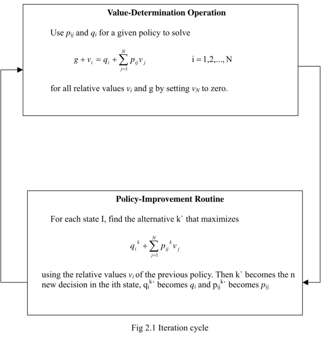
We have now, by somewhat heuristic means, described a method for finding a policy that is an improvement over our original policy. In [1] it proves that the new policy will have a higher gain that the old policy. First, however, we shall show how the value-determination operation and the policy-improvement routine are combined in an iteration cycle whose objective is to find a policy that has highest gain among all possible policies. The basic iteration cycle may be diagrammed as shown in Fig. 2.1
Fig 2.1 Iteration cycle
The upper box, the value-determination operation, yields the g and v i
corresponding to a given choice of p andij q . The lower box yields the i p and ij q i
that increase the gain for a given set of v . In other words, the value-determination i
operation yields values as a function of policy, whereas the policy-improvement routine yields the policy as a function of the values.
We may enter the iteration cycle in either box. If the value-determination operation is chosen as the entrance point, an initial policy must be selected. If the
Value-Determination Operation
Use pij and qi for a given policy to solve
N 1,2,..., i 1 = + = +
∑
= N j j ij i i q p v v gfor all relative values vi and g by setting vN to zero.
Policy-Improvement Routine
For each state I, find the alternative k` that maximizes
∑
= + N j j k ij k i p v q 1using the relative values vi of the previous policy. Then k` becomes the n
new decision in the ith state, qik` becomes qi and pijk` becomes pij.
cycle is to start in the policy-improvement routine, then a starting set of values is necessary. The selection of an initial policy that maximizes expected immediate reward is quite satisfactory in the majority of cases.
At this point it would be wise to say a few words about how to stop the iteration cycle once it has done its job. The rule is quite simple: The final robust policy has been reached (g is maximized) when the policies on two successive iterations are identical. In order to prevent the policy-improvement routine from quibbling over equally good alternatives in a particular state, it is only necessary to require that the old d be left unchanged if the test quantity for that i d is as large as that of any i
other alternative in the new policy determination.
In summary, the policy-iteration method just described has the following three properties:
1. The solution of the sequential decision process is reduced to solving sets of linear simultaneous equations and subsequent comparisons.
2. Each succeeding policy found in the iteration cycle has a higher gain than the previous one.
3. The iteration cycle will terminate on the policy that has largest gain attainable within the realm of the problem; it will usually find this policy in a small number of iterations.
These three properties are proved in [1].
In contrast to a simple demultiplexing protocol like UDP, TCP is a more sophisticated transport protocol that can provide a reliable, connection-oriented, byte-stream service, and is widely used to reliably transfer data in computer network. It has a window based congestion-control mechanism to keep the sender from overloading the network. TCP never sends more than one window size of packets into the network. This window size is controlled by a mechanism, which is commonly called AIMD (additive increase/ multiplicative decrease). The basic idea of the AIMD mechanism is that TCP keeps increasing the size of congestion window, which limits how many packets can be transmitted per round trip time (RTT), until it detects that a packet has been dropped.
There are several different implementations of TCP, like RENO, TAHOE or new RENO. In our simulation, all of our traffic sources use RENO TCP to send data packets. RENO TCP includes four mechanisms: slow start, congestion control, fast retransmit and fast recovery. Its congestion window is controlled by slow start and congestion control. At the beginning, RENO TCP transmits packet with slow start mechanism, and each ACK from destination increases congestion window by one. Until a packet has been dropped in the network, so the destination receives an out of order packet and it sends an ACK packet with the last in order packet’s sequence number to the source. Then the fast retransmit mechanism will retransmit the missing packet and TCP now uses the congestion control mechanism to transmit packet.
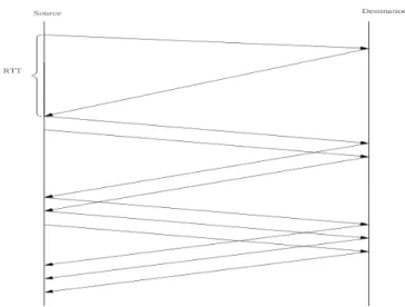
Fig 2.2 Packets in transit during additive increase, with one packet being added each RTT
The Fig 2.2 shows the behavior of the TCP while it still uses slow start to transmit packet, that means each ACK from destination triggers the source to send two more packets. According to Fig 2.3, the traffic rate generated by the “Source” might be considered as the product of the congestion window size and packet size divide by the value of round trip time. But in general, the round trip time is much larger than the transmission time, that means the TCP sender generates a short period of burst traffic per round trip time.
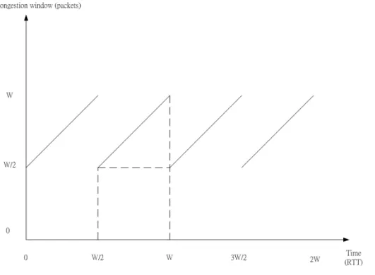
Fig 2.3 TCP window evolution under periodic loss. Each cycle delivers p w w 1 ) 2 ( 2 1 ) 2
( 2+ 2 = packets and takes
2
w round trip times
TCP sender’s throughput is actually depending on the packet drop probability of the network. In [4], a simplified model of the throughput of a single TCP connection has been established. The author makes the following assumptions,
1.TCP connection has infinite data to send.
2.A TCP source is running over a lossy path which has a constant round trip time
(RTT), because it has sufficient bandwidth and low enough total load that it never
sustains any queues
3. Approximating random packet loss at constant probability p by assuming that the link delivers approximately 1/p consecutive packets, followed by one drop 4.The maximum value of the window is W.
as fig (2.3) and the relation between the throughput of the source and the drop probability p can be described as
p C BW RTT MSS = (2.12)
The constant of proportionality (C) lumps together several terms that are typically constant for a given combination of TCP implementation, ACK strategy (delayed v.s. non-delayed), and loss mechanism. In Eq (2.12), MSS denotes maximum segment size. But in practice, there are much more than one TCP connections passing through a single router or a gateway. Even we know the number of the TCP connections which are passing through the router or a gateway, the relation between the total throughput and the drop probability will not be the multiplication of the Eq (2.12) and the number of TCP connections. But it is believed that the total throughput of the TCP connections is direct proportion to the square root of the drop probability deployed by the router.
2.3 Explicit Congestion Notification (ECN)
TCP infers that the network is congested from a packet drop, which is indicated by retransmit timer timeouts or duplicate acknowledgements. This mechanism can be an expensive way to detect network congestion. An alternative way for routers or other network devices to inform TCP senders that network is congested is using ECN (explicit congestion notification). ECN enhances active queue management, like RED,
packets are marked rather than dropped. As such, congestion information can be quickly transferred to the source host where the transfer rate can be immediately adjusted without additional delay in waiting for a duplicated ACK or timeout. As a result, unnecessary packet drops can be avoided.
In general, TCP should respond to a single marked packet as it would to a lost packet. That means TCP cuts down the congestion window by halve and reduces the slow start threshold. The next four sections summarize the modifications TCP need to implement ECN.
2.3.1 ECN-TCP header
To cooperate with ECN, TCP needs two additional bits in the header: one to indicate
that the connection is ECN capable (ECT-bit) and another to indicate network congestion (CE-bit). If a connection uses ECN for congestion control then the ECT-bit is set to 1 for all packets, otherwise it is set to 0. How a gateway decides which packet to mark is according to what kind of active queue management mechanism it uses.
Furthermore, ECN introduces two new flags in the reserved field of the TCP header. One of them is the ECN echo flag, which is set in an ACK packets by the receiver if an data packet’s CE-bit has been set. The other flag is the congestion window reduced (CWR) flag. This flag is set by the sender after it has reduced its congestion window for receiving congestion notification.
Gateways may use various kinds of active queue management mechanism, like RED or BLUE [8]. Gateways supporting ECN can choose to mark arriving packets instead dropping them.
2.3.3 ECN-TCP Sender
The sender treats an ECN echo ACK as a lost packet, but without the need to retransmit the marked packet. Although this ACK acknowledges a data packet, it does not increase the congestion window. If the sender receives multiple congestion indications, including timeouts, duplicate ACKs and ECN echo ACK, it should react just one per RTT to the congestion indication. In the case that a retransmitted packet is marked or dropped, the sender reacts to congestion indication again. After the sender responds to a congestion indication, it sets the CWR flag in the next data packet sent after the reduction of the window.
2.3.4 ECN-TCP Receiver
The receiver echoes the congestion notification of a CE packet back to the sender.
The receiver will keep setting every ACK packet’s CE bit to 1 until it receives a data packet with the CWR flag has been set to 1 from sender. This provides robustness in case an ACK packet with the echo flag set gets lost.
RED is an active queue management mechanism that is intended to address some of the shortcomings of standard tail-drop FIFO queue management [3]. In a FIFO queue it is possible for “lock-out” to occur, a condition in which a small subset of the flows sharing the link can monopolize the queue during periods of congestion. Flows generating packets at a high rate can fill up the queue such that packets from flows generating packets at substantially lower rates have a higher probability of arriving at the queue when it is full and being discarded. A second problem with a FIFO queue is that latency is increased for all flows when the queue is constantly full. Simply making the queue shorter will decrease the latency but negates the possibility of accommodating brief bursts of traffic without dropping packets unnecessarily. RED addresses both the lock-out problem by using a random factor in selecting which packets to drop and the “full queue” problem by dropping packets early, before the queue fills.
RED monitors router’s queue length and when it detects that congestion is imminent, it notifies the source to adjust its congestion window by dropping packets. RED is invented by Sally Floyed and Van Jacobson in [2]. It has been designed to be used in conjunction with TCP. The authors say that their goal is to avoid a bias against bursty traffic. Networks contain connections with a range of burstiness, and gateways such as Drop Tail and Random Drop gateways have a bias against bursty traffic. With Drop Tail gateways, the more bursty the traffic from a particular connection, the more likely it is that the gateway queue will overflow when packets from that connection arrive at the gateway.(2)
The basic idea of RED is shown in Fig (2.4) algorithm RED 2.4 Fig packet arriving mark the max if else packet arriving mark the : p y probabilit with p y probabilit calculate max min if size queue average the calculate arrival packet each for th a a th th avg avg avg < < <
In addition to Fig (2.4), RED needs two more algorithms : one for calculating the average queue length, one for calculating drop probability. RED uses the following equation to calculates the drop probability :
max ) min (max ) min ( y probabilit drop p th th th avg p − − = (2.13)
and maxp denotes the maximum probability which is used by RED to drop (or mark)
the packet. Eq (2.14) is used to calculate the average queue length
avg=wq ⋅avg+(1−wq)⋅q (2.14)
We now summarize RED’s behavior as follows : when a packet arrives to the router, RED calculates the value of the average queue size (avg) according to the current queue size (q) by using Eq(2.14), then uses it to find the drop (or mark) probability
The authors of [2] classify the network congestion in to two kinds: longer-lived congestion and transient congestion. The transient congestion increases the size of the queue temporarily while the longer-lived congestion increases the average queue length. Among all connections passing through the router, some connections may generate more bursty traffic than others, so these connections are more likely to cause transient congestion to happen. Some other congestion control methods, like Random Drop or Drop-Tail mechanisms, have bias against to burst traffic. By adjusting probability according to the average queue length, Sally and Van believe that RED is able to avoid the bias against bursty traffic.
Finally, RED is claimed to provide several benefits, in particular 1) decrease the end-to-end delay for both responsive (TCP) and non necessarily responsive real-time traffic (UDP), 2) prevent large number of consecutive packet losses by ensuring available buffer space even with bursty traffic, and 3) remove the higher loss bias against bursty traffic observed with Tail Drop.
It has been believed that the performance of RED is highly depending on the value of the parameters: maxth , minth , maxp and wq. But it is vary difficult to configure
these parameters. In [10], several different experiments have been done to examine RED’s performance with different parameter settings. It concludes that RED parameters have a minor impact on the performance with small buffer and using RED with large buffer indeed can improve the system’s performance.
results in a significant decrease of the drop rate suffered by bursty traffic only when the fraction of bursty traffic is small. Otherwise, the main effect of RED is to increase the drop probability of smooth traffic without improving the drop probability of the bursty traffic, comparing to Tail drop mechanism. In practice, if we replace "bursty" with 'TCP" and "smooth" with "interactive UDP audio" for example, and if we note that TCP makes up the vast majority of Internet traffic, the result above means that the overall loss rate suffered by TCP connections when going from Tail Drop to RED will not change much, but that the loss rate suffered by UDPLIP telephony applications (whether they are rate adaptive or not) will increase significantly.
2.5 Motivation
In this section, we first discuss the difficulty of implementing RED. We now know that RED is controlled by five parameters: maxth , minth , maxp, wq and buffer size. But
we didn’t show how to set these parameters. We now discuss it in two different criteria. In [6], they discuss the stability of throughput of TCP connections while the bottleneck link is using RED. They use the average size of all TCP connections’ congestion windows as an indicator of stability. It shows that even all TCP connections have the identical round trip time, the average size of the congestion windows still can oscillate heavily, which means the systems is unstable, if the round trip time is large. It is because that the traffic from TCP connections only appears a short period of time per RTT, which means that there is only transient congestion but no longer-lived congestion and RED tries not to respond to such kind of congestion. In RED, the parameter wq is used to control the sensitivity to the duration of periods of
delay is larger than 140ms, the size of the average window oscillates heavily. In [6], they conclude that it is the protocol stability more than other factor that determines the dynamic of TCP/RED. But it is very difficult to develop a new protocol and ask every one to use it. So, instead of modifying TCP, finding a way to improve RED’s stability seems to be more practical.
Another way to discuss the stability of TCP/RED is to examine the stability of the router’s queue length. While system is stable, the instantaneous queue length oscillates between minth and maxth. In [7], the stability of the queue length has been analysed and a necessary condition has been proposed as follows. Let C denotes the link capacity (packets/sec), N denotes the number of TCP sessions , R denotes round trip time and
δ ) 1 ( log K , min max e max q th th w P L = − − = ,
where δ is the sampling time, see [9]
Then, for K and L satisfy the following condition, the queue length will be stable.
} 1 , 2 min{ 1 . 0 where 1 ) 2 ( ) ( 2 2 2 2 3 R C R N w K w N RC L g g = + ≤ .
In general, different TCP session will have different round rip time. So in [7], it mentions that we can use an equivalent round trip time to see if the condition could be satisfied. In fact, in the presence of heterogenous round trip times for the flows, this bound should be interpreted for what we call the equivalent round trip time of the flows. The equivalent round trip is calculated as the harmonic means of the individual
round trip time of the flows. Consider a scenario with N flows having heterogenous round trip times Ri. The harmonic mean of the round trip times (Req) is given by
=
∑
N i eq N R R 1 1 1 1 .From above condition, we can see that the stability of TCP/RED is related to the network environment. However, how these parameter settings affect the bandwidth utility and average queuing delay is unidentified. Also, the information of network environment, like the numbers of TCP session and round trip time of each TCP connection are not easy to get, and changing all the time. So it is generally considered that the major difficulty in deploying RED is how to set its parameters.
According to the previous section, we know that if we want to stabilize TCP/RED performance, we need to know more information about network environment, like the number of TCP sessions, round trip time per session or equivalent round trip time. Some people may try to make RED to dynamically tune these parameters by itself, like “Adaptive RED algorithm”[11] or “Auto-Tuning algorithm” [12]. But all these methods still use queue length as an indicator of network congestion. We agree with that buffer is always needed because TCP session generates bursty traffic and routers need buffer to contain such burst. But we want to try a more aggressive way to do the congestion control on routers by controlling the packet arrival rate observed at the router, so the router can maintain low buffer occupation and maximize the bandwidth utility at the same time. Also, we want to conclude the effect caused by different network environments to just one parameter, so the mechanism can be vary easy to
Chapter 3
Self-Configurable Congestion Control
In this chapter we are going to develop our method, which can maintain the packet
arrival rate to be 95% of link’s bandwidth in different network environments and maintain the low buffer occupation. Here, the “different network environments”
means “the different combinations of the TCP sessions’ round trip times”. We first separate the problem into two parts: the first part is how to achieve our goal, the second part is to tune our method according to the network environment.
Since Markov decision process is a convenient tool to find a policy according to the state space and cost function, which are defined according to our purpose. So we will use the Markov decision process to control the packet arrival rate, and find a way to compensate the difference between the reality and our Markov model. Before building up the model, we first discuss what kind of problem we are dealing with. First, we assume that we can directly control TCP senders’ throughput with some error by sending some kind of ‘rate command’ to them. To simplify the problem, we also assume that all TCP senders have the same round trip time. Once we detect that the arrival rate is higher then we expected, we shall ask TCP senders to decrease their throughput lower than the desired value, so the buffer occupation can be decreased. And to raise the throughput if the current arrival rate is lower than we want. We need to know when to raise (lower) the throughput and how much to raise (lower) it. We will use Markov Decision Process to solve this problem.
In reality, TCP senders will respond to packet drops or “marked” ACK packets (if ECN is implemented) and decrease their throughput. So the “rate command” is given in the form of packet drop probability. We need three mechanisms to achieve our goal, one to generate policy according to different error, one to determine the effect of the error, and one to find out the relation between drop probability and packets arrival rate.
3.1 Model for MDP
We use MDP to generate our desired policy and we will start to build a Markov decision process to generate our desired policy from now on. We first define the discrete state space as the packet arrival rate, since our goal is to control the packet arrival rate, which is measured in the percentage of the target bandwidth. Let S denotes the state space, then S={10,20, ... ,200}, which represents 10% to 200% of target bandwidth. And we assume at each state, we can give “rate commands” to control TCP sessions’ throughput. We define these “rate commands” to be our action space A, A={15,25,35,45,50,60,76,86,90,94,95,96,97,98,99,105,110,120,130,140}. Each action represents the amount of the target bandwidth (measured in percentage).
An essential part of Markov is the state transition probability, but such kind of transition probability of TCP traffic is very hard to determine. Instead of using complicated model, we try to build up a simplified model that can satisfy our need. Another important issue is that we shall conclude the effect of real network environment on just one parameter, so we can let the model to configure this parameter by its own self to reduce the difference between our model and the reality.
Obviously, there is no such technique can help us to build up our model, and such kind of model has not yet been seen. So we build a model that can generate our desired policy first, then we analyze our model later to see if it is reasonable. We conclude the properties of our policy as follows: 1. While the arrival rate is larger than 100% of bandwidth, we should ask TCP senders to decrease their throughput lower than 100% of bandwidth to decrease the queue length; 2. While the arrival rate is smaller than 100% of bandwidth, we should ask TCP senders to increase their throughput larger than 100% of bandwidth to increase the queue length; 3. By changing just one parameter, the Markov decision process should be able to generate a new policy. We use MDP to decide when to decrease the rate and how much should it decrease. We try to use normal random variables to generate state transition probability. The reason of choosing normal random variable is that we can easily control its mean and deviation to generate our desired policy.
After merely infinite trials, we conclude that state transition probability for a transition from state i to state j by choosing action k ( k
ij
P ) should be in the following
form: (3.1) 20 j for , -1 1 j for , ]] [ [ 19 j 2 for , )] 2 ] 1 [ ] [ ( ) 2 ] 1 [ ] [ [( 19 1 j
∑
= = = = ≤ = ≤ ≤ + + ≤ < − + = k ij k i k i k ij p j state N p j state j state N j state j state p Pand the variable k i
N denotes the normal random variable we used to generate
(3.3) . * ) 1 ( * ] [ 100 deviation (3.2) ] [ * ) 1 ( ] [ * mean k i α α σ α α μ error k action i state k action k i = − − + − + =
The parameter α and error are used to represent the effect of the real network environment, and we can configure the value of them to reduce the difference between our model and the reality. We will explain their roles and functionality later. And the immediate cost is defined to be :
] [
100 statei
rij = − . (3.4)
So we are looking for a policy that can minimize the cost. Such policy will keep arrival rate approaching to 100% of target bandwidth. If we set α to be 0.9 and
error to be 40, then we can use the method introduced in section (2.1) to find the
policy. In general, it takes only 5 iterations to find the policy. The result is shown in table (3.1)
State 10 20 30 40 50 60 70 80 90 100 110 120 130 140 150 160 170 180 190 200 Action 105 105 105 105 105 99 99 99 99 99 99 99 99 99 99 98 97 95 94 94
Table(3.1) policy obtained by iteration method forα=0.9, error=40
And the lost of the Markov process is 28.730847. This means that under such policy in average the instantaneous packet arrival rate is about [1+
−(0.28730847)]*(target
bandwidth). We try to maintain the average packet arrival rate to be the target bandwidth by using policy that can minimize the lost. And simply by changing the
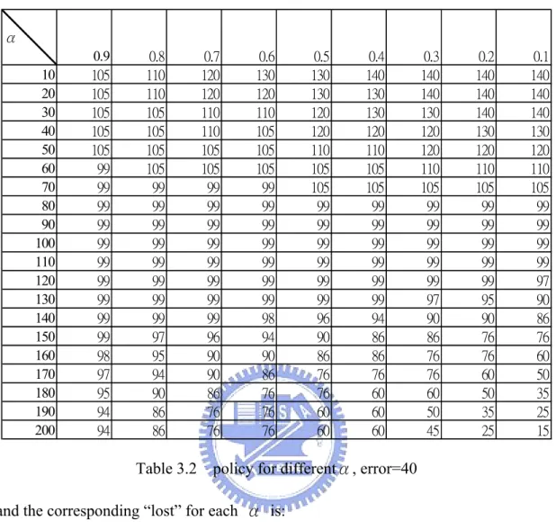
value ofα, we can generate different policy as in Table (3.2). α 0.9 0.8 0.7 0.6 0.5 0.4 0.3 0.2 0.1 10 105 110 120 130 130 140 140 140 140 20 105 110 120 120 130 130 140 140 140 30 105 105 110 110 120 130 130 140 140 40 105 105 110 105 120 120 120 130 130 50 105 105 105 105 110 110 120 120 120 60 99 105 105 105 105 105 110 110 110 70 99 99 99 99 105 105 105 105 105 80 99 99 99 99 99 99 99 99 99 90 99 99 99 99 99 99 99 99 99 100 99 99 99 99 99 99 99 99 99 110 99 99 99 99 99 99 99 99 99 120 99 99 99 99 99 99 99 99 97 130 99 99 99 99 99 99 97 95 90 140 99 99 99 98 96 94 90 90 86 150 99 97 96 94 90 86 86 76 76 160 98 95 90 90 86 86 76 76 60 170 97 94 90 86 76 76 76 60 50 180 95 90 86 76 76 60 60 50 35 190 94 86 76 76 60 60 50 35 25 200 94 86 76 76 60 60 45 25 15
Table 3.2 policy for differentα, error=40 and the corresponding “lost” for each α is:
α 0.1 0.2 0.3 0.4 0.5 0.6 0.7 0.8 0.9 “lost” 9.4158 11.6888 13.9770 16.2859 18.6062 20.9794 23.4336 26.0079 28.7308 Table 3.3 “lost” value of different α
From table(3.2), we can see that for largerα, the policy becomes more aggressive. So if current state is much larger than target bandwidth, the policy will decrease the TCP senders’ throughput significantly.
In our model, we have two parameter need to be configured: α and error. However, our current technique can only dynamically adjust one of them. Because that a different policy correlates to a different value of ‘lost’. So, we can use the value of gain to connect between the Markov process and the real network environment. For example, we can first assume the error is very large, so we let α to be 0.91 and use Markov decision process to find the policy. Then we use the policy to control the arrival rate and record the immediate cost as the system transits between states. After a while, we can obtain the real value of the system’s lost, and we can use this value to find the corresponding value of α. Then, we can use the new α to find a new policy. We define g to be the average of immediate cost t
over time, so gt is actually the “lost” of the Markov process, and update g in the t
following way: t r g g gt = t−1+ t−1− t (3.5)
In eq(3.5), t denotes the number of stages, and r denotes the immediate cost we t
observed at stage t. So after we obtain the new value of g , we will find the value t
ofα according to the table (3.3) and generate a new policy.
3.3 Calculate Drop probability
update rule to tune our Markov decision process according to the real network. So the last thing we have to do is to find out the relation between drop probability and TCP senders’ throughput. From eq(2.12) , we define C' to be :
p BW
C'=⋅ ⋅ (3.3)
We findC' according to the history. We record the packet arrival rate and drop
probabilities we deployed in the past 500ms. Let rateavg denotes the average
packet arrival rate in the past 500ms, and pavg denotes the average drop
probability in the past 500ms. Now we can use C' to calculate the corresponding
drop probability for each action :
dropprobability [ '/(target bandwidth*action/100)]2
C
= . (3.4)
For example, by setting target bandwidth to be 50, which means 50 Mbytes/sec, and
'
C to 10, then table (3.2) can be translate into table (3.4). Under this assumption,
the corresponding drop probability of the action ‘15’ is larger then 1, which is unreasonable. So we limit the maximum drop probability to be 0.8.
α 0.9 0.8 0.7 0.6 0.5 0.4 0.3 0.2 0.1 10 0.036 0.033 0.028 0.024 0.024 0.02 0.02 0.02 0.02 20 0.036 0.033 0.028 0.028 0.024 0.024 0.02 0.02 0.02 30 0.036 0.036 0.033 0.033 0.028 0.024 0.024 0.02 0.02 40 0.036 0.036 0.033 0.036 0.028 0.028 0.028 0.024 0.024 50 0.036 0.036 0.036 0.036 0.033 0.033 0.028 0.028 0.028 60 0.041 0.036 0.036 0.036 0.036 0.036 0.033 0.033 0.033 70 0.041 0.041 0.041 0.041 0.036 0.036 0.036 0.036 0.036 80 0.041 0.041 0.041 0.041 0.041 0.041 0.041 0.041 0.041 90 0.041 0.041 0.041 0.041 0.041 0.041 0.041 0.041 0.041 100 0.041 0.041 0.041 0.041 0.041 0.041 0.041 0.041 0.041 110 0.041 0.041 0.041 0.041 0.041 0.041 0.041 0.041 0.041 120 0.041 0.041 0.041 0.041 0.041 0.041 0.041 0.041 0.043 130 0.041 0.041 0.041 0.041 0.041 0.041 0.043 0.044 0.049 140 0.041 0.041 0.041 0.042 0.043 0.045 0.049 0.049 0.054 150 0.041 0.043 0.043 0.045 0.049 0.054 0.054 0.069 0.069 160 0.042 0.044 0.049 0.049 0.054 0.054 0.069 0.069 0.1 170 0.043 0.045 0.049 0.054 0.069 0.069 0.069 0.1 0.16 180 0.044 0.049 0.054 0.069 0.069 0.1 0.1 0.16 0.327 190 0.045 0.054 0.069 0.069 0.1 0.1 0.16 0.327 0.64 200 0.045 0.054 0.069 0.069 0.1 0.1 0.198 0.64 0.8
Table 3.4 drop probability for differentα, error=40
For example, if we change drop probability every 1 ms, according to how many packets arrived in the past 1ms, then the mechanism can be shown in fig (3.1)
probability every 1ms according to it. We use p_history[i] and rate_history[i] to record the drop probability we deployed and packet arrival rate, and calculate the average rate and average drop probability over past 500 ms according to the record.
3.4 MORE about Markov model
We will explain the function of a special term ‘error’ in our Markov model in this section. This term appears in the transition probability, and need to be set manually. The relation between the ‘lost’ and the value of ‘error’ is shown in table (3.5)
error 10 20 30 40 50 60 70 80 range of 'lost' for α=0.1~0.9 0.58 ~6.96 4.50 ~14.34 7.58 ~21.59 9.41 ~28.73 11.11 ~35.44 12.72 ~41.47 14.28 ~46.71 15.81 ~51.20 Table (3.5) Range of ‘lost’ of different α.
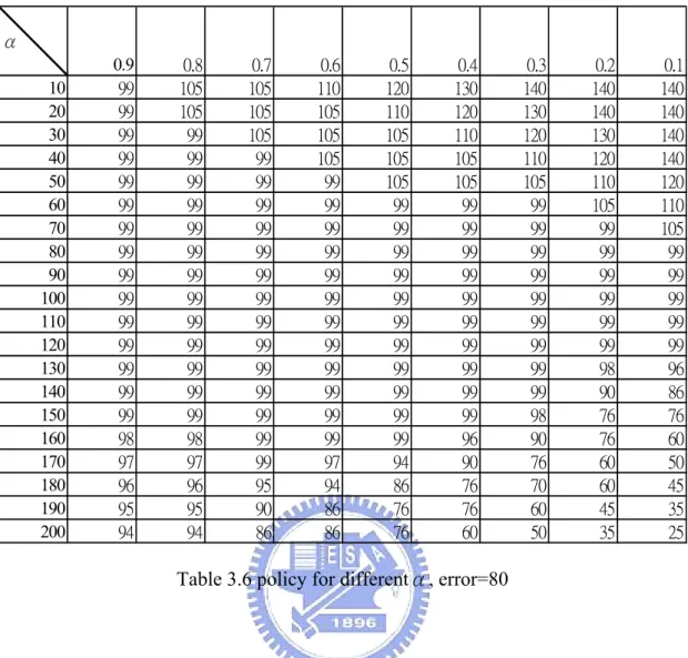
So we can see that the parameter ‘error’ can be used to choose the range of lost. If the error is set to be too small, our self-configuring mechanism will not work. For example, controlling the packet arrival rate to be maintained in the range of (1± 6.96%) target bandwidth seems to be not possible. So we suggest that the value of error should be set larger than 40. The table (3.6) shows the policy while error is 80.
α 0.9 0.8 0.7 0.6 0.5 0.4 0.3 0.2 0.1 10 99 105 105 110 120 130 140 140 140 20 99 105 105 105 110 120 130 140 140 30 99 99 105 105 105 110 120 130 140 40 99 99 99 105 105 105 110 120 140 50 99 99 99 99 105 105 105 110 120 60 99 99 99 99 99 99 99 105 110 70 99 99 99 99 99 99 99 99 105 80 99 99 99 99 99 99 99 99 99 90 99 99 99 99 99 99 99 99 99 100 99 99 99 99 99 99 99 99 99 110 99 99 99 99 99 99 99 99 99 120 99 99 99 99 99 99 99 99 99 130 99 99 99 99 99 99 99 98 96 140 99 99 99 99 99 99 99 90 86 150 99 99 99 99 99 99 98 76 76 160 98 98 99 99 99 96 90 76 60 170 97 97 99 97 94 90 76 60 50 180 96 96 95 94 86 76 70 60 45 190 95 95 90 86 76 76 60 45 35 200 94 94 86 86 76 60 50 35 25
Table 3.6 policy for differentα, error=80
We start to analyze our model now by discussing the mean. As we can see, if α is larger, the mean dependents on our action more than our current state.
Chapter
4
Simulation
In this chapter, we describe our simulator and simulated network topology. Our simulator is designed by using Rhapsody version 5.01.
4.1 UML Simulator design
The object model diagram of our simulator is shown in Fig (4.1).
Fig(4.1) Object model diagram of our simulator
The class ‘tcp’ is modified from two files of NS version 2.29 :tcp.cc, tcp-reno.cc. Despite the TCP protocol, a traffic generator and a duplex link with infinite sized buffer also specified in the class ‘tcp’. Basically, we can replace the following representation of NS by using a single instance of ‘tcp’ class.
$ns duplex-link $n0 $n2 2Mb 10ms DropTail set tcp [new Agent/TCP/Newreno]
$ns attach-agent $n0 $tcp set ftp [new Application/FTP] $ftp attach-agent $tcp $ftp set type_ FTP
The class ‘Sink’ is designed to ACK each TCP packets. The size of its receiving buffer is designed to be 200 packets. It also has ability to support ECN technology. Like the ‘tcp’ class, it also includes a duplex link with infinite sized buffer in it. The following representation of NS can be replaced by a single instance of the class ‘sink’:
set n4 [$ns node]
$ns duplex-link $n3 $n4 0.5Mb 40ms DropTail set sink [new Agent/TCPSink]
$ns attach-agent $n4 $sink
The class ‘link’ specifies a simplex link with finite buffer in NS. It also specifies an RED algorithm from [2] to perform congestion control. This function can be disabled, so the buffer is simply controlled by tail drop mechanism. The following representation of NS can be replaced by a single instance of the class ‘link’:
$ns simplex-link $n2 $n3 0.3Mb 100ms DropTail
The ‘packet’ class is used to simulate the network packet in the real world. It uses an array to record each link it has to passing through to reach the destination. And it also has necessary attributes that can be used to support ECN.
The instance of ‘sysclock’ class not only counts time, but also links to each instances of class ‘tcp’, ‘sink’ and ‘link’. It routes packet through links to its destination (TCP sender or sink receiver) according to the rout information recorded on the ‘packet’. Finally, the ‘markov’ class specifies our proposed congestion control
congestion control.
4.2 Network topology
Fig (4.2) network model
Consider Fig (4.1), there are several TCP senders sending data packet through a bottleneck link L1, and TCP sinks sending ‘ACKs’ back through L2. Each of L1 and L2 uses an AQM (active queue management ) method to control the length of queue. We assume that L2 has a sufficient large capacity and uses FIFO to manage the buffer, so ‘ACKs’ from TCP sinks will never be marked or dropped. Also, we assume that links t1,t2,..,tN and s1,s2,..,sN have very large capacity. The above assumption
guarantees that TCP senders sense a packet drop event only because that a data packet has been dropped by L1’s AQM or buffer overflowed on L1. We also assume that delays of links t1,t2,…,tN and s1,s2,…sN, may be different so each TCP session may
have different round trip time. If we can control the aggregate traffic rate from TCP senders T1 to TN to be 95% of link L1’s bandwidth, then the queue length of L1 will
be small almost every time.
In our simulation, all of our senders using RENO TCP with ECN support to provide congestion control, which is implemented according to ns2. And sink will ‘ACK’ to each packet. Our senders can generate two different kinds of traffic with fixed packet size: short burst traffic and persistent traffic. Senders generate persistent traffic will keep sending packets as many as congestion window allowed. Sender generates short burst traffic sends 11 packets at first, after receiving all the ‘ACKs’ it waits an exponential distributed random time with a mean of 350 msec then sends another 11 packets. We implement our congestion control mechanism as L1’s AQM, and L2’s buffer is simply controlled by FIFO. During all our experiment, the L1’s bandwidth is set to be 50 Mbytes and the L2’s bandwidth is set to be 100 Mbytes. So, it takes 20μsec for L1 to transmits a data packet and 10μsec for L2 to transmits an ‘ACK’packet. We also set the bandwidths of links t1,t2,…,tN and s1,s2,…sN to be 100
Mbytes. The maximum size of queue of L1 is 1000 packets. And the maximum size of queue of L2 is set to be very large to guarantee that the ‘ACK’ packets will never be dropped.
4.3 simulation results
In this section, we demonstrate how different environments affect the performance of TCP/RED and proposed congestion control mechanism. RED parameters is set as follows : packets. 1000 size buffer , 02 . 0 w packets, 50 min packets, 750 max , 1 . 0 max th th q = = = = = p
RED and our congestion control mechanism under several different network environments to demonstrate that while RED’s performance is highly dependent on the environment, our mechanism can always keep good performance.
4.3.1 Identical delay
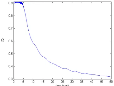
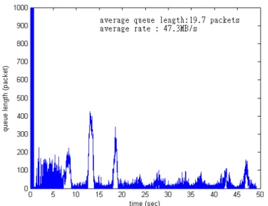
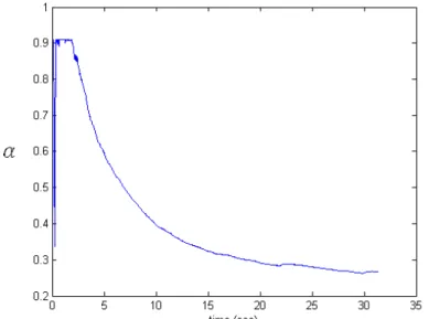
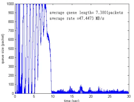
In the first experiment, we use 200 TCP sessions with identical delays to test TCP/RED’s performance. This experiment shows how different round trip delays can cause critical effect to TCP/RED’s performance. In the first case, we set the round trip delay to be 40 ms. Under this condition, TCP/RED’s performance is quit well, it achieve 100% bandwidth utility and control the average queue length at 156.2 packets. But our mechanism can do even better, our mechanism control the average queue length at 6.09 packets and bandwidth utility is 95%. In the second experiment, we set the round trip time to be 140ms. The result shows in Fig 5.6, although the average queue length is maintained at 56.5 packets, and no buffer overflow happens after it become stable. But the bandwidth utility is down to 74.8% of bottleneck link’s bandwidth. Our mechanism still can maintain the 95% bandwidth utility and the average queue length is maintained at 19.7 packets. From these two experiments, we can see that RED
Fig 4.3 value of α of 200 TCP sessions with 40msec round trip time (Proposed mechanism)
Fig 4.4 queue status of 200 TCP sessions with 40ms round trip time (Proposed mechanism)
Fig 4.5 queue status of 200 TCP sessions with 40ms round trip time (RED)
Fig 4.7 queue status of 200 TCP sessions with 140msec (Proposed mechanism)
Fig 4.8 queue status of 200 TCP sessions with 140ms round trip time (RED)
4.3.2 Different amount of TCP session
As mentioned in the previous chapter, TCP/RED’s stability and performance can be improved by increasing the number of TCP sessions. So we fixed the round trip time to be 140 ms, and increase the number of TCP sessions to see how the performances of TCP/RED and our mechanism are affected by it. Unlike RED, our mechanism can
maintain the average queue length at a very small value even the amount of TCP sessions increases to 1000. But when the number of TCP sessions is small, the average queue length is higher. We briefly explain this behavior as follows: Assume the bottleneck link’s bandwidth is equally shared by all sessions, then from eq (2.1) we can get that the proper drop probability for maintaining the bandwidth utility at 95% is less then 8*10−4, with such small drop probability, the packets are rarely
being marked, so the average queue length can be a larger. And from fig (5.6), fig (5.8) and fig (5.11), we can see as the number of TCP sessions increases, the average queue length and throughput increase, too. TCP sessions’ throughput depends on the packet mark (drop) probability it suffers over all the links it passes through.
Fig 4.9 value of α of 1000 TCP sessions with RTT=140ms (Proposed mechanism)
Fig 4.10 queue status of 1000 TCP sessions with RTT=140ms (Proposed mechanism)
Fig 4.11 queue status of 1000 TCP sessions with RTT=140ms
Fig 4.12 value of α of 500 TCP sessions with RTT=140ms
Fig 4.13 queue status of 500 TCP sessions with RTT=140ms (Proposed method)
Fig 4.14 queue status of 500 TCP sessions with RTT=140ms (RED)
4.3.3 Heterogeneous delays
In this experiment, we set the TCP sessions to have different round trip delays (in the range of 30msec~140msec). This is more like real network environment than identical delays. Under this situation, things get more complicated. In the previous experiments, we see that for 140ms round trip delay, theα should be 0.3 . Since for the same drop probability, each TCP session now generate different throughput, so our congestion control suffer larger noise now. As a result, the maximum value of instantaneous queue size and average queue size all becomes larger, but the average throughput still can maintain at 95% of bottleneck link’s bandwidth.
Fig 4.15 value of α queue status of 100 TCP sessions with round trip delay=30~140 msec
Fig 4.16 queue status of 100 TCP sessions with round trip delay=30~140 msec (Proposed method)
Fig 4.17 queue status of 100 TCP sessions with round trip delay=30~140 msec (RED)
Fig 4.19 queue status of 500 TCP sessions with round trip delay=30~140 msec (Proposed method)
Fig 4.20 queue status of 500 TCP sessions with round trip delay=30~140 msec (RED)
4.3.4 With and without update mechanism
In the last experiment, we show that the update mechanism indeed can find the proper policy. We use 500 TCP sessions with heterogeneous delays in the range of 30~140 msec, and the same settings of our mechanism as in section 3.4. But we choose the value ofα manually, and fixed them for all time. The result is shown in
becomes smaller. Obviously, when the drop probability is too large, the throughput becomes smaller than we want. With the help of our update mechanism, our congestion control can fin the proper policy that can maintain 95% of bandwidth utility.
α
state 0.1 0.6 0.9 update average queue
length 22.3632 40.082 47.45 37.2 average arrrival rat40.5MB/s 46.4MB/s 45.2MB/s 47.2MB/s Table 4.1 performance of our mechanism with and without update mechanism
Chapter 5
Conclusion
Since RED has been published, a lot of researchers try to analyze its behavior, and dozens of ways about how to tune RED’s parameters have been announced. There are also many different forms of RED-like congestion control algorithms have been proposed. However, all of them focus on controlling the queue length and use queue-based control mechanism to avoid buffer overflow, which leads them to nowhere. RED claims that it can provide many benefits like avoiding synchronization, avoiding buffer overflow, and providing some kind of fairness, but it has never been widely deployed. In this thesis, we focus on controlling the arrival rate instead of queue length. The idea is that if we can maintain the arrival rate to be 95% of link’s bandwidth, then buffer occupancy should be low or zero. Such kind of rate-based congestion control has not yet been developed because the difficulty on modeling TCP’s throughput. It can be very difficult to build up a math model that captures the characteristics of real TCP’s throughput behavior. However, it is much easier to build up a model for MDP to generate a policy that satisfies some general concepts. In this thesis, we develop a simplified model for MDP and an assistant mechanism that can minimize the difference between our simplified model and the reality. The result shows that our algorithm indeed can outperform RED on maintaining the low buffer occupancy and high bandwidth utility.
References
[1] Ronald A. Howard, “Dynamic Programming and Markov Process”
[2] Sally Floyd and Van Jacobson, “Random Early Detection Gateways for congestion Avoidance”, IEEE/ACM Transactions on Networking, August, 1993.
[3] B. Braden, D. Clark, J. Crowcroft, B. Davie, S. Deering, D. Estrin, S.Floyd, V.Jacobson, G. Minshall, C. Partridge, L. Peterson, K. Ramakrishnan, S. Shenker, J. Wroclawski, and L. Zhang, “Recommendations on queue management and congestion avoidance in the Internet,”, RFC2309, Apr. 1998.
[4] Mathis, M., Semke, J. Mahdavi, J. and Ott, T.J. (1997), “The Macroscopic Behavior of the TCP Congestion Avoidance Algorithm”. Computer
Communications Review 27 (3), pp 67 - 82 (July 1997).
[5] Martin May, Thomas Bonald, and Jean- Chrysostome Bolot, “Analytic evaluation of RED performance,” in Proceedings of IEEE infocom, March 2000
[6] Steven H .Low, Fernando Paganini, Jiantao Wang, Sachin Adlakha, John C.Doyle, “Dynamics of TCP/RED and a Scalable Control” , Proceedings of IEEE Infocom, June 2002
Theoretical analysis of RED”, IEEE infocom 2001.
[8] W. Feong, D.Kandlur, D.Saha, and K. Shin, “The Blue active queue management algorithms”, IEEE IEEE/ACM Transactions on Networking (TON) Volume 10, Issue 4 (August 2002) Pages: 513-528, 2002.
[9] Vishal Misra, Don Towsley and Wei-Bo Gong, “Fluid based Analysis of a network of AQM Routers supporting TCP Flows with an Application to RED” in Proceedings of ACM/SIGCOMM. 2000
[10] Martin May, Jean Bolot, Christophe Diot, and Bryan Lyles, “Reasons not to deploy RED”, In Proc. of 7th Int. Workshop on Quality of Service
(IWQoS ’99), London, pages 260–262, June 1999.
[11] W.-C. Fmg, D.D. Kandlur, D. Saha, and K.G. Shin, "A Self Configwing RED Gatnuay:' Pmceedingr of IEEE INFOCOM '99, pp. 1320 -1328, Mar 1999. Eiahteenth Annual Joint Confcmee of the IEEE Computer and Communication Societies
[12] Harsha Sirisena, Aun Haider and Krzysztof Pawlikowski, “Auto-Tuning RED for Accurate Queue Control”, Global Telecommunications conference, 2002, IEEE