兆赫波段可調式液態晶體Solc濾波器

國

立

交

通

大

學

光電工程學系

碩

士

論

文

       

兆赫波段可調式液態晶體 Solc 濾波器

A Liquid-Crystal-Based Terahertz Tunable Solc Filter

 

       

研 究 生：何宜貞

指導教授：潘犀靈 教授

   

中 華 民 國 九 十 六 年 七 月

兆赫波段可調式液態晶體 Solc 濾波器

A Liquid-Crystal-Based Terahertz Tunable Solc Filter

 

研  究  生：何宜貞      Student：I-Chen Ho 

指導教授：潘犀靈      Advisor：Ci-Ling Pan 

 

 

國  立  交  通  大  學 

光  電  工  程  學  系 

碩  士  論  文 

 

A Thesis

Submitted to Institute of Electro-Optical Engineering & Department of Photonics College of Electrical and Computer Engineering

National Chiao Tung University in partial Fulfillment of the Requirements

for the Degree of Master

in

Photonics July 2007

Hsinchu, Taiwan, Republic of China

兆赫波段可調式液態晶體 Solc 濾波器

學生：何宜貞

指導教授

：

潘犀靈

國立交通大學光電工程學系﹙研究所﹚碩士班

摘

要

我們研製了一種兆赫波段可調式

Solc 濾波器，實驗數據與理論預

測相符合。利用外加磁場控制向列型液晶(E7)的雙折射性，可在室溫下

連續調變穿透頻率從

0.176 至 0.793 THz (中心頻率之調幅可達 350%)；

此濾波器之置入能量損耗為

5dB。為了改善置入能量損失、使用便利

性與快速反應等因素，我們也設計了一種電場控制向列型液晶(E7)之

Solc 濾波器，在室溫下連續可調範圍從 0.717 到 1.142 THz (中心頻率

之調幅可達

59%)。我們也量測具較大雙折射性(Dn~0.18)向列型液晶

(DN125262W) 的折射係數並利用此材料製作 Solc 濾波器，與 E7 相同

濾波效果下，此濾波器操作在較低頻區(< 0.7 THz)，置入性損耗減少

~1.5 dB。

A Liquid-Crystal-Based Terahertz Tunable Solc Filter

student：

I-Chen Ho

Advisors：Dr.

Ci-Ling Pan

Department (Institute) of Photonics

National Chiao Tung University

ABSTRACT

A large tunable range, room-temperature terahertz Solc filter has been

demonstrated. The first central pass-band frequency of the device can be

continuously tuned from 0.176 to 0.793 THz (a fractional tuning range of

350%) using magnetically controlled birefringence in the nematic liquid

crystals (E7). The insertion loss of the present device is about 5 dB. We

also designed and constructed an electrically controlled, tunable terahertz

Solc filter of which the central pass-band frequency can be continuously

tuned from 0.717 to 1.142 THz (a fractional tuning range of 59%). The

electrically tuned filter has advantages of compact use, ease in control, fast

response, and low insertion loss. Moreover, we have investigated a

commercial liquid crystal DN125262W with large birefringence and

applied it for filtering applications. It can operate at low frequencies (< 0.7

THz).and the insertion loss reduce ~1.5dB, comparing with E7. The results

are in good agreement with theoretic predictions.

誌

謝

何其榮幸能在交大度過兩年的碩士生學習，對這裡的一切充滿著極大

的不捨，潘犀靈教授亦師亦父的教導和趙如蘋教授無私的提供實驗與

技術上的指導，使我能更深的進入科學的核心。然而實驗室的博士班

學長們，以及同學與學弟妹，更是讓我在每天的生活中充滿驚奇與樂

趣，尤其難忘的是碩一修課時，和同學們討論作業與合作找資料的成

就感。

更感謝父母在我求學生涯的支持與關心，雖然是耳提面命也是我最

甜蜜的支柱。當然還有紹文姊姊，謝謝妳讓我每天拖著疲憊的身體回

家時，可以完全的放鬆自己。最後謝謝正凱，你總是在我最需要幫助

的時候，犧牲自己的時間使我能做到最好，希望你也能達成你的夢想。

宜貞 2007/7/24

Contents

Abstract (Chinese) I

Abstract (English) II

Acknowledgements III

Contents IV

Tables VI

List of Figures VII

Chapter 1. Introduction 1

1.1. Terahertz technology: Terahertz Filter 2

1.2. Nematic Liquid Crystal 3

1.3. Thesis highlights 6

1.4. References 8

Chapter 2. Terahertz Time-domain-spectroscopy (THz-TDS) 10

2.1. Introduction 10

2.2. Schematic setup of THz-TDS radiation using PC antenna 10

2.3. Generation of THz radiation Using PC antenna 14

2.4. Detection of THz-TDS radiation using PC antenna 16

2.5. The application of THz-TDS: extracting the refractive index of a

large birefringence LC-DN125262W 19

Chapter 3. Magnetically Controlled Liquid-Crystal-Based Terahertz

Tunable Solc Filter 27

3.1. Introduction 27

3.2. Theory of Solc filter 28

3.3. Design and measurement 30

3.4. Results 35

3.5. Discussion 39

3.6. Comparison with our previous work: a THz Lyot filter 41

3.7. Summary 42

3.8. References 43

Chapter 4. Electrically Controlled Liquid-Crystal-Based Terahertz

Tunable Solc Filter 45

4.1. Introduction 45

4.2. Previous evaluation 45

4.3. Sample preparation and setup 46

4.4. Results and discussion 50

4.5. A four-stage folded cascaded Solc filter 53

4.6. Improvement 55

4.7. Summary 56

4.8. References 57

Tables

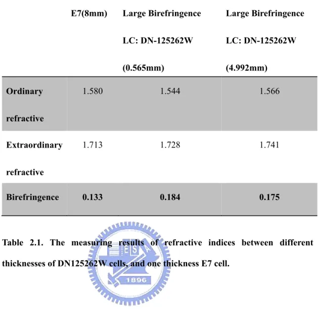
Table 2.1. The measuring results of refractive indices between different thicknesses of

DN125262W cells, and one thickness E7 cell. 25

List of Figures

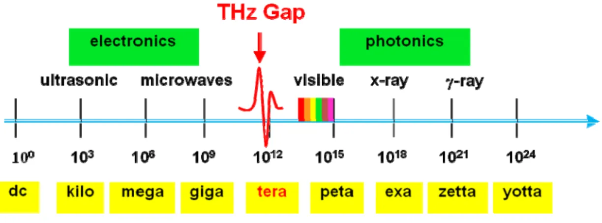
Fig. 1.1. The diagram defines the name of electromagnetic wave in different frequency

ranges. 1

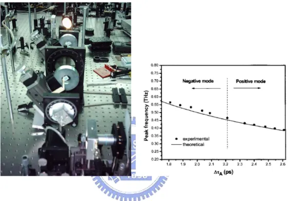
Fig. 1.2. (a) The experimental diagram of the LC-based tunable THz Lyot filter. (b) The peak transmitted frequencies of the filter vs different time delay,

Δ

τ

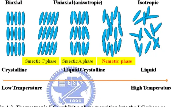
_A. The circles are experimental data and the curve is theoretical prediction 3

Fig. 1.3. Thermotropic LCs exhibit a phase transition into the LC phase as temperature is changed. 4

Fig. 1.4. The three types of deformation occurring in nematics. The figure shows how each type may be obtained separately by suitable glass walls. 5

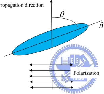
Fig. 1.5. The angle,θ, between the director of LC molecules and the propagation direction of incident light will affect the effective index of extraordinary wave. 6

Fig. 2.1. LT-GaAs PC antenna 11

Fig. 2.2. Schematic diagram of the transmission-type THz-TDS system. 12

Fig. 2.3. The results of the THz signal passing through the air. (a) and (b) are time domain waveforms with and without purge; (c) and (d) are frequency domain spectrum with and without purge, respectively. 14

Fig. 2.4. THz detector. 16

Fig. 2.5. The sketches of reference cell (a) and the LC cell (b). 19

Fig. 3.1. A six-stage folded Solc filter 28

Fig. 3.2. The light path mechanism after passing six half wave plates. 28

Fig. 3.3. Schematic diagram of the LC-based tunable THz Solc filter. The inset (a) and (b) show two different ways to apply magnetic field on the same tunable LC THz retarders, respectively. 32

Fig. 3.4. Experimental setup of the LC-based tunable THz Solc filter. The Fig. (a) and

(b) refer to the schematic diagram in Fig. 3.3 (a) and (b), respectively. 33

Fig. 3.5. An example of the transmittance of the broadband THz pulse through LC Solc

filter filled with E7. The circles are experimental data and the solid line is theoretical prediction. 35

Fig. 3.6. An example of the transmitted spectrum of the broadband THz pulse which is

tuned using a LC (E7) THz Solc filter. The insert is time domain profiles. The circles and squares are experimental data and the solid lines are the theoretical prediction. 36

Fig. 3.7. The first-order central frequencies of the filter filled with E7 versus rotation

angle θ between magnetic field and z axis. The circles are experimental data. The curve is theoretical calculation. 37

Fig. 3.8. An example of the transmitted spectrum of the broadband THz pulse through

LC Solc filter filled DN125262W. The circles are experimental data and the solid line is theoretical prediction. 38

Fig. 3.9. The central transmitted frequencies of the filter filled with DN125262W versus

rotation angle θ between magnetic field and z axis. The circles are experimental data. The curve is theoretical. 38

Fig. 3.10. The temporal profiles of a THz pulse through (a) E7 based Solc filter and

reference LC cells (b) DN125262W based Solc filter and reference ones. 40

Fig. 4.1. The simulation results of electirc field distribution between electrodes in an

empty LC cell (a) in a lateral view (b) in a top view. 46

Fig. 4.2. The schematic diagram of homeotropical alignment LC cell. The cell gap is

1.5mm. 47

Fig. 4.3. The schematic diagram of one element in a tunable LC THz Solc filter. The

propagation direction of the THz wave is along Z axis. The direction of applied electrical field is tilted with 22.5° or -22.5° referring to X axis. 47

Fig. 4.4. The experimental picture of the two folded THz Solc filter based on LCs. 48

Fig. 4.5. The schematic diagram of LC molecules orientating under different fields. Ec

is the threshold voltage and E is the applied field. 49

Fig. 4.6 Spectra of the transmitted broadband THz pulse through the LC THz Solc filter

at several voltages. The circles, diamonds and squares are experimental data and the solid lines are the theoretical prediction. 51

Fig. 4.7. The central transmitted frequencies of the filter versus applied voltages. The

circles are experimental data. The curve is theoretical line. 52

Fig. 4.8. Solc filters consist of wave plates of two thicknesses. The circles and squares

are experimental data. The curves are theoretical prediction. 53

Fig. 4.9. The schematic diagram of a tunable four folded cascaded THz Solc filter. 54

Fig. 4.10. Spectra of the transmitted broadband THz pulse through the four folded Solc

Chapter1. Introduction

In these twenty years, resplendent progress in terahertz (THz) wave field has been made. THz frequency locates between microwave and visible which is shown in Fig. 1.1. The development of solid-state femtosecond lasers and advanced optoelectronic THz-devices promote a new era of fundamental and applicable THz science. THz studies ranging from investigations of ultrafast dynamics in materials to biological media and three dimensional imaging have been actively explored. For today and future applications in THz science, quasi-optic components such as filters are indispensable.

However, there are shortages of optical components in the THz frequency range. Most THz tunable devices such as filters have the problems with small tunable range and cryogenic operating temperature. More recently, we have demonstrated the both electrically and magnetically controlled liquid-crystal (LC) THz phase shifter [1,2]. Here, we propose to study and design the THz Solc filter by using LC retarders. The purpose is to solve the current lack of the THz wavelength filter with large tunable range.

In this chapter, the background information on our recently survey of THz Filter, and the background information of Nematic LCs (NLCs) are presented. The structure of the thesis is presented in the last part of this chapter as “Thesis highlight”.

1.1 Terahertz technology: Terahertz Filter

Ultrafast optoelectronic technology has been developed for these decades, and many applications of THz spectroscopy are exploited. Many quasi-optic components such as phase shifters, attenuators, polarizers, and filters are in high demand. Recently, several types of tunable THz filters have also been demonstrated. These include: a tunable THz attenuator and filter (operating at cryogenic temperature) based on a mixed type-I/type-II GaAs/AlAs multiple quantum well structure tuned by optical injection [3]; by using of SrTiO3 as a defect material inserted into a

periodic structure of alternating layers of quartz and high-permittivity ceramic, a photonic crystal filter tuned from 185 GHz at 300 K down to 100 GHz at 100 K [4]; some groups using voltage controlled wavelength selection at microwave frequencies by zero-order grating with LCs [5]; a metallic hole arrays or photonic crystals (MHA or MPC) filter made tunable over the range of 365-386 GHz by a relative lateral shift of 140 μm between two micro-machined MPC plates [6], control of enhanced THz transmission through two dimensional MHA using magnetically controlled birefringence in NLCs [7]and a magnetically controlled LC based THz tunable Lyot filter with tunable range from 0.388 to 0.564 THz [8].

The magnetically controlled LC based THz tunable Lyot filter was demonstrated and published in Applied Physics Letters in March 2006 by our group

previously. This filter is the first time a tunable room-temperature THz filter. Fig. 1.2 (a) and (b) are the experimental arrangement and the peak transmitted frequencies of Lyot filter vs different time delay,

Δ

τ

_A. However, considering practicability and functionality, we demonstrate a THz tunable Solc filter in this thesis.

Fig. 1.2. (a) The experimental diagram of the LC-based tunable THz Lyot filter.

(b) The peak transmitted frequencies of the filter vs different time delay,

Δ

τ

_A. The circles are experimental data and the curve is theoretical prediction.

1.2 Nematic Liquid Crystal

The first observation of liquid crystalline or meso-morphic behavior was made near the end of 19th century by Reinitzer and Lehmann [9, 10]. LCs are substances that exhibit a phase of matter with properties between a conventional liquid, and a solid crystal. Therefore, a LC may flow like a liquid, but has the molecules in the

which can be distinguished based on their different optical properties (such as birefringence). LCs can be divided into thermotropic and lyotropic LCs. Thermotropic LCs exhibit phase transition into the LC phase as temperature is changed (Fig. 1.3), whereas lyotropic LCs exhibit phase transition as a function of concentration of the mesogen in a solvent (typically water) as well as temperature.

Fig. 1.3. Thermotropic LCs exhibit a phase transition into the LC phase as

temperature is changed.

Thermotropic LCs includes smectic phase, nematic phase, chiral phase, and discotic phases. However, nematic phase is most common investigated; the LCs utilized in our work is all rod-like nematic LCs, where the molecules have no positional order, but they have long-range orientational order. Most nematics are uniaxial: they have one axis labeled as a unit vector (or director), with the other two being equivalent (can be approximated as cylinders). Some LCs are biaxial nematics, meaning that in addition to orienting their long axis, they also orient along a secondary axis.

Fig. 1.4. The three types of deformation occurring in nematics. The figure

shows how each type may be obtained separately by suitable glass walls.

(Reproduced from P. G. de Gennes and J. Prost, The Physics of Liquid

Crystals, 2nd ed. , Oxford, New York, 1983).

We also can use some boundary conditions, add chiral dopant, or apply external field (magnetic or electrical field) to rearrange LC molecules. For a uniaxial system, single crystal, the molecules along one common direction ≤

nˆ

in an ideal. Three types of the deformation (splay, twist, and bend) occur in nematic phase as shown in Fig. 1.4 [11]. Briefly, the LC molecules tend to orient parallel or perpendicular to the external field and the extra energy density is a function of the direction and magnitude of the field. Besides, the LC molecules around a strong boundary condition will be aligned and twisted due to the lowest total energy.

As mentioned above, nematic LC molecules tend to be parallel to the director composing an optically uniaxial system where the refractive index is birefringence. The ordinary index no is for light with polarization perpendicular to the director,

whereas the extraordinary index ne is for light with polarization parallel to the

nˆ

Propagation direction 

θ

 

If the incident polarization of light has tilt angle with respect to the director, the refractive index of extraordinary wave should be rewritten as:

2 1 2 2 2 // 2 ) cos sin ( − ⊥ + = n n n_eff θ θ (1.2) where θ is the angle between the propagation direction of incident light and the optical axis as shown in Fig. 1.5.

Fig. 1.5. The angle,θ, between the director of LC molecules and the propagation direction of incident light will affect the effective index of extraordinary wave.

1.3. Thesis highlights

In chapter 2, we depict the schematic setup of THz Time Domain Spectroscopy (THz-TDS) radiation using photoconductive (PC) antenna, and explain the

generation and detection principles of THz-TDS radiation with PC antenna. Then, the characteristics of radiation and detection in our TDS system are discussed.

Finally, we extracted the refractive index of E7 (Merck) and a new LC: DN125262W Polarization

(daily polymer corporation) in THz range via THz-TDS system.

In chapter 3 and 4, a magnetically controlled LC-based THz tunable Solc filter and an electrically controlled LC-based THz tunable Solc filter have been reported, respectively. We design various structures of the LC based filter to get extensive applications in THz range. Finally, we give a conclusion in chapter 5.

1.4. References:

1. C.Y. Chen, C.F. Hsieh, Y.F. Lin, R.P. Pan, and C.L. Pan, Magnetically tunable room-temperature 2p liquid crystal Terahertz phase shifter., Opt. Express, 12, 2630-2635 (2004).

2. C.F. Hsieh and R.P. pan, T.T. Tang, H.L. Chen, and C.L. pan,” Voltage-contralled liquid-crystal terahertz phase shifter and quarter-wave plate,” Opt. Lett.,

31,1112-1114 (2006).

3. I. H. Libon, S. Baumgärtner, M. Hempel, N. E. Hecker, J. Feldmann, M. Koch, and P. Dawson, “An optically controllable terahertz filter,” Appl. Phys. Lett. 76, 2821-2823 (2000).

4. H. Nemec, P. Kuzel, L. Duvillaret, A. Pashkin, M. Dressel, M. T. Sebastian, “ Highly tunable photonic crystal filter for the terahertz range,” Opt. Lett., 30, 549-551 (2005).

5. F. Yang and J. R. Sambles, “Microwave liquid crystal wavelength selector,” Appl. Phys. Lett., 79, 3717-3719 (2001).

6. T. D. Drysdale, I. S. Gregory, C. Baker, E. H. Linfield, W. R. Tribe, D. R. S. Cumming, “Transmittance of a tunable filter at terahertz frequencies,” Appl. Phys. Lett. 85, 5173-5175 (2004).

7. C.-L. Pan, C.-F. Hsieh, and R.-P. Pan , M. Tanaka, F. Miyamaru, M. Tani, and M. Hangyo, “Control of enhanced THz transmission through metallic hole arrays using nematic liquid crystal,” Opt. Express 13, 3921-3930 (2005).

8. C.-Y. Chen, C.-L. Pan, C.-F. Hsieh,Y.-F. Lin, and R.P. Pan, “Liquid-crystal-based terahertz tunable Lyot filter,” Appl. Phys. Lett. 88, 101107 (2006)

9. R. Reinitzer, "Zur Kenntnis des Cholesterins," Monatsh. Chem. 9, 421-441 (1888). 10. O. Lehmann, "On flowing crystals," Z. Phys. Chem. 4, 462 (1889).

11. P. G. de Gennes and J. Prost, The Physics of Liquid Crystals, 2nd ed. (Oxford, New

York, 1983).

Chapter2. Terahertz

Time-domain-spectroscopy (THz-TDS)

2.1. Introduction

Investigations of LC filters in the THz frequency range utilized THz time domain spectroscopy (THz-TDS). THz-TDS is a powerful technique allowing broadband THz generation and detection of field amplitude and phase. Various techniques is used to generate THz radiation, such as ultrafast switching of photoconductive antennas [1], rapid screening of the surface field via photoexcitation of dense electron hole plasma in semiconductors[2], rectification of optical pulses in crystals[3], and carrier tunneling in coupled double-quantum well structures[4]. However, photoconductive (PC) antennas have a promising source of intensity and spectral bandwidth.

Therefore, in this chapter we discuss photoconductive emitter and detector antennas in THz-TDS system in Sec.2.2 and deduce the generation and detection principles of photoconductive antennas in Sec.2.3 and Sec.2.4. Finally, we extract the refractive index of a large birefringence LC-DN125262W by using THz-TDS system in Sec.2.5.

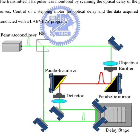
2.2. Schematic setup of THz-TDS radiation using PC antenna

Low –temperature grown GaAs (LT-GaAs) was used as the PC substrate for generation and detection of THz waves. The material has great advantages of short

carrier life time, reasonably high mobility, and high break down electrical field. A PC antenna with a pair of square stab at the center of a coplanar transmission line on LT-GaAs was used for an emitter and a detector (Fig. 2.1).

Fig. 2.1. LT-GaAs PC antenna

A mode-locked Ti: sapphire laser (Spectra Physics Tsunami) is the light source to excite PC antennas. The pulse width and the repetition rate of the laser were 50 fs and 82 MHz, respectively. The pulses are split into two beams: one is the so-called pump or excited beam; the other is referred as the probe beam. A schematic representation of our system is depicted in Fig. 2.2. Pump pulse were focused on the biased gap of the dipole-type LT-GaAs PC antenna, which results in conductivity in the gap varying in subpicosecond time scale.

The transient variation of conductivity caused the transient electrical current in the gap, leading to generation of THz radiation. Average power of pump pulse is about 35 mW and 5 volt is applied to the coplanar transmission line. A hemispherical silicon substrate lens attached to the antenna to avoid the multiple reflections within the SI-GaAs substrate. The generated THz pulses are collected and guided by a pair of gold-coated parabolic mirrors. The incident THz waves on the sample can be

by another parabolic mirror onto the detector of dipole-type LT-GaAS PC antenna also attached a hemispherical silicon substrate lens. The Ti:sapphire laser probe pulse impinged on LT-GaAs generating charge carriers and effectively turned on the antenna for a short time interval. Average power of probe pulse is 15mW and time interval typically is a few hundreds of femtoseconds determined by the lifetime of the excited carriers. Transient current was induced in the gap of the detector antenna with the focused THz electric field, which accelerated the photocarriers excited by the probed beam. PC current signal, with 5 kHz-modulation of the bias applied to emitter, was synchronously detected by a digital lock-in amplifier equipped with a current-voltage preamplifier module (Stanford Research Systems, Model SR830). The transmitted THz pulse was monitored by scanning the optical delay of the probe pulses; Control of a stepping motor for optical delay and the data acquired were conducted with a LABVIEW program.

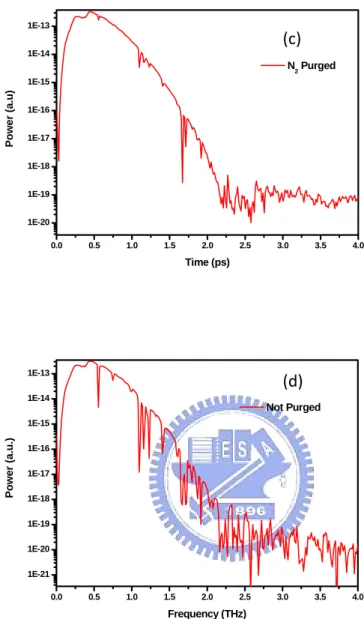
The diameter of the THz beam was ~ 8 mm, the total scanning duration of the THz was 68 ps, and the measurements were done at room temperature (25±0.5°C). Fig. 2.3 is the results of the THz signal passing through the air with purge and without purge. Apparently, the pulse after main signal is smooth in purge condition while the pulse after main signal fluctuates severely in no purge condition due to water absorption referring to Fig. 2.3 (a) & (b). As to frequency domain, the

spectrum in Fig. 2.3 (d) has many absorption lines of water below 2 THz, comparing with the spectrum in Fig. 2.3 (b). Besides, the power spectrum extends to 2THz and its the signal/noise is up to 107, which is a well performance system to measure many characteristics of devices. 0 10 20 30 40 50 60 -0.0006 -0.0004 -0.0002 0.0000 0.0002 0.0004 0.0006 0.0008 N 2 Purged Am plit ude ( a .u.) Time (ps) 0 10 20 30 40 50 60 -0.0006 -0.0004 -0.0002 0.0000 0.0002 0.0004 0.0006 Not Purged A m pli tude (a .u.) (a)  (b) 

0.0 0.5 1.0 1.5 2.0 2.5 3.0 3.5 4.0 1E-20 1E-19 1E-18 1E-17 1E-16 1E-15 1E-14 1E-13 N 2 Purged Pow e r (a. u ) Time (ps) 0.0 0.5 1.0 1.5 2.0 2.5 3.0 3.5 4.0 1E-21 1E-20 1E-19 1E-18 1E-17 1E-16 1E-15 1E-14 1E-13 Not Purged Power (a .u .) Frequency (THz)  

Fig. 2.3. The results of the THz signal passing through the air. (a) and (b) are

time domain waveforms with and without purge; (c) and (d) are frequency

domain spectrum with and without purge, respectively. 

2.3. Generation of THz radiation Using PC antenna

When a biased semiconductor is pumped by an ultrafast laser pulse, the rapid change of the transport photocurrent gives rise to electromagnetic radiation. The following calculation is based on Drude-Lorentz theory of carrier transports in

(c) 

semiconductors [5]. When the carrier is pumped by ultrashort laser pulse, the time dependence of carrier density is given by:

G n dt dn c + − = τ _(2.1) where n is the density of the carrier, G is the generation rate of the carrier by the

laser pulse, and τ_c is the carrier trapping time.

Again, the generated carriers can be accelerated in biased electrical field. The acceleration of carriers is given by:

E m q v dt dv h e h e s h e h e , , , , _{=− +} τ (2.2)

where ve,h is the average velocity of the carrier, qe,h is the charge of an electron (a

hole), me,h is the effective mass of an electron (a hole), τs is the momentum

relaxation time, and E is the local electrical field, which is less than the applied

bias E due to the screen effect of space charges. More precisely, _b

αε

P E

E= _b − (2.3) where P is the polarization induced by the spatial separation of the electron and

hole, ε is the dielectric constant of the substrate, and α is the geometrical factor of photoconductive material, which is equal to three in isotropic dielectric material. The time dependence of polarization P can be written by:

J P dt dP r + − = τ (2.4) where τ_r is the recombination time between an electron (τ_r=10 ps for LT-GaAs) and a hole and J =envh −enve is the current density.

t v en t n ev t J E_THz ∂ ∂ + ∂ ∂ ∝ ∂ ∂ ∝ (2.5)

where v=v_h −v_e is a relative speed v between an electron and a hole

Therefore, the transient electromagnetic field E_THz is composed of two parts: one is due to carrier acceleration under the electric field, and the other is due to the change of carrier density.

2.4. Detection of THz-TDS radiation using PC antenna

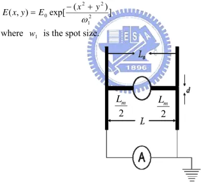
For the detection of THz field, which is a Gaussian beam on the detector expressed as [6]: ] ) ( exp[ ) , ( ₂ 1 2 2 0 ω y x E y x E = − + (2.6)

where w₁ is the spot size.

Fig. 2.4. THz detector.

The total resistance over the detector is:

td L td L L R= ρM M +ρs S ≈ ρs S _(2.7)

where L_M is the total length of the mental electrodes, L is the length of the S

switch area between the two electrodes tips, ρ and _M ρS are their resistivity, 2 m L 2 m L

respectively, and d is the width of electrode and the gap area as shown in Fig. 2.4. The average resistivity ρ_S is larger than ρ due to the low duty cycle of the _M driving laser (100 fs/10 ns = 5

10− ). The resistivity ρ_S depends on photogenerated carrier density, which for homogeneous illumination of power Plaser scales as:

laser S S P d L ξ ρ = (2.8)

where ξ is a conversion factor between laser power and number of photogenerated carriers.

The average electric field E across the detector gives rise to a potential difference

) (LM LS

E

U = + , so the average current is

laser S S M P td L L L E R U I = = ( ₂+ ) ξ (2.9)

The average electric field across the detector area is

) 2 ( ) 2 ( ) , ( 1 ) , ( 1 1 2 1 0 2 2 2 2 ω ω πω d Erf L Erf Ld E dy dx y x E Ld d L E d d L L = =

_∫

_∫

− − (2.10) where Erf =

∫

χ −u du π χ 0 2₎ exp( ) 2 ( )

( is an error function. The peak strength of the electric field, E , can be expressed in terms of the total power of THz beam: ₀

2 0 0 2 1 2 0 2 1 ) , ( 2 1 E c dy dx y x E c PTHz = ε

∫

∫

= πω ε ∞ ∞ − ∞ ∞ − (2.11) 0 1 2 0 2 ε π ω c P E = THz ⇒ (2.12)

Besides, for wavelength

L

R

2 0

πω

λ<< , however, the lens is cut to place the detector

gap at the position given by

1 − = n n R h _L (2.13)

where RL is the lens radius and n is the index of refraction of the lens material.

Justifying the lens design:

1 lim 0 = − > − _n n R d_{focus L} λ 1 1 ) ( lim 0 0 1 0 = − = − > − _n R c n R d L L focus _{πω πνω} λ ω λ (2.14) Where λ ν = c is the frequency.

By inserting Eq. (2.12), together with Eq. (2.14), into the expression for the detector current, Eq. (2.9), we get

⎥ ⎦ ⎤ ⎢ ⎣ ⎡ − ⎥ ⎦ ⎤ ⎢ ⎣ ⎡ − − = πω ν πω ν ν ω πε ξ ν L L S L Thz laser cR n d Erf cR n L Erf n d L t R cP P I 0 0 0 2 0 ) 1 ( 2 ) 1 ( 2 1 ) 1 ( 2 ) ( (2.15)

In short, the time domain signal I(ν)relative to the emitted THz electric field

E and the response function of the detector. The carrier life time of LT-GaAs, transmission characteristics of the SI-GaAs substrate and LT-GaAs film, resonance characteristics of dipole-type antenna, diffraction effect of the THz beam optics, and pulse widths of probe beam, etc, all contribute to the transient response function of the detector.

2.5. The application of THz-TDS system: extracting the

refractive index of a large birefringence LC-DN125262W

The knowledge of the frequency dependence and the magnitude of the refractive indices as well as the birefringence of liquid crystal is a key parameter for practical applications of LCs. Although many groups have investigated the birefringence of LCs in visible or infrared range, we expect a large birefringence with low loss LCs in THz range.

For searching high birefringence LCs, we measure the refractive index of a large birefringence LC_DN125262W, a special mixture from daily polymer corporation, by using THz-TDS to determine it. We prepared two cells: the reference cell is constructed by two fused silica substrates contacting each other; each LC cell is constructed by two fused silica substrates separated by an aluminum spacer and filled with DN125262W as shown in Fig 2.5. The inner surfaces are coated with polyimide films, which are baked and rubbed to give LCs the homogeneous alignment. LC  Alignment  Direction  (a)  Reference Cell  THz beam  LC Cell  THz beam  Fused Silica 

(b) 

The Polarization of Incident THz Wave: e‐ray      ; o‐ray 

If a plane wave pass through the cell normally, the electric field of the THz wave through the reference cell at angular frequency,ω , can be written as

) , ( ) ( ) ( ) ( E0 P d E_reference ω = ω ⋅η ω ⋅ _air ω (2.16)

where E₀(ω)is the electric field of THz wave before passing through the cell, )

(ω

η is a coefficient including all the reflection, transmission and propagation coefficients in fused silica and Pair( dω, )is the propagation coefficient in air, which

dis the thickness of the LC layer. Generally, for a medium over a distance L, the

propagation coefficient P_a(ω,L)can be written as exp[(−in~_aωL)/c], where n~_a

(=na −iκ) is the complex refractive index of medium a, which depends on the wave

frequency. In η(ω), the echoes of the THz wave or Fabry-Perot effect in fused silica can be neglected since in the thick sample, these echoes are far away from the main signal on the time domain and can be truncated during the spectrum analysis. The electric field of a THz wave passing through the LC cell is given by:

)

,

(

)

(

)

,

(

)

(

)

(

)

(

)

(

E

₀

T

P

d

T

F

d

E

_LC

ω

=

ω

⋅

η

ω

⋅

_q−LC

ω

⋅

_LC

ω

⋅

_LC−q

ω

⋅

_LC

ω

(2.17) where Ti−j(ω)is the transmitted Fresnel factor of i− jinterface, which is

) ~ ~ /( ) ~ 2 ( ) ( i i j j i n n n

T₋ ω = ⋅ + and Fa(ω,L)is the Fabry-Perot effect in a medium with

thickness L. Because of the same thickness of fused silica substrates used in this work, η(ω)is equal to the reference cell. The complex transmission coefficient

) (ω

T of the measured LC as follow:

) ( ] ) ~ ~ ( exp[ ) ~ ~ ( ~ ~ 4 ) ( ) ( ) ( ₂ ω ω ω ω ω LC air LC q LC q LC ref LC F c d n n i n n n n E E T ⋅ − − ⋅ ⋅ + ⋅ ⋅ = = (2.18)

where n~q is the complex index of fused silica and n~LCis the ordinary index o

a

o n i

demonstrated the solutions in 1996 for optically thick and thin samples [7]. Here, we make thick sample to simplify the analysis processes such that the echoes of THz waves from multiple reflections of sample are temporally well separated from main signal. So F_LC(ω)in Eq. 2.18 can be equal to 1.

If we let the reference cell have an empty gap of the same thickness of LC cell, the

) (ω F will be rewritten as ) ~ ~ ( ) ~ ~ ( ) ~ ~ ( ) ) ~ ~ ( 2 exp( ) ~ ~ ( ) ~ ~ ( ) ~ ~ ( ) ( q air q LC LC q air LC q LC q air air q LC n n n n n n c d n n i n n n n n n F + ⋅ − ⋅ − − ⋅ + ⋅ − ⋅ − = ω ω (2.19)

Instead of solving n~_LC from T(ω)−T_meas(w)=0, where T(ω) and T_meas(ω)are

respectively the calculated and measured complex transmission coefficients, we define an error function, δ(n,κ), and then find (n,κ)by minimizing the error

function. The error function is defined as :

2 2 ) , ( κ δρ δϕ δ n = + (2.20)

whereδ =ln(T(ω))−ln(Tmeas(ω)) (2.20a)

δϕ =arg(T(ω))−arg(Tmeas(ω)) (2.20b)

After several iterations to minimize the error function by computer programs, we get the refractive indices as following results:

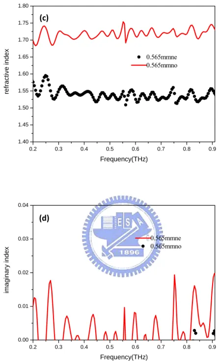
We repeated four times of measurements in the LC cell with 4.992 mm cell gap where to get the same result in each one. Fig. 2.6 (a) is the result of extraordinary and ordinary refractive indices, and (b) is the result of imaginary extraordinary and ordinary refractive indices of DN125262W with 4.992mm cell gap. Besides, we also fabricated DN125262W LC cells with 0.565mm cell gap, and Fig. 2.6 (c) is

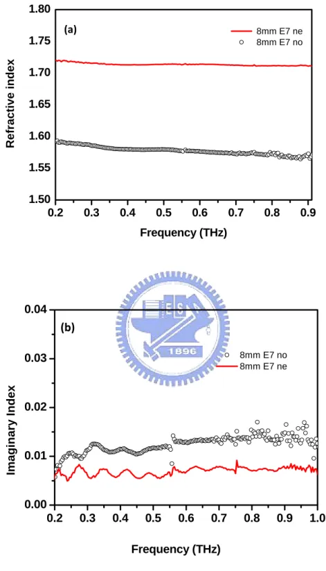
ordinary refractive indices, shown as a function of frequency from 0.2 to 0.95 THz. Comparing with the refractive index of E7, Fig. 2.7. (a) and (b) are the refractive indices of E7 with 8mm cell gap, measured by our group before. Therefore, the birefringence of DN125262W is larger than E7, which largely enhances applications to wave plates or filters. Table 2.1 is a comparison of two kinds of LC molecules according to our measurement.

0.2 0.3 0.4 0.5 0.6 0.7 0.8 0.9 1.5 1.6 1.7 1.8 4.992mm ne1 4.992mm ne2 4.992mm no1 4.992mm no2 Refractive in d e x Frequency(THz) 0.2 0.3 0.4 0.5 0.6 0.7 0.8 0.9 0.00 0.01 0.02 0.03 0.04 4.992mm no1 4.992mm no2 4.992mm ne1 4.992mm ne2 im ag in ary i n d ex Frequency(THz)    (a) (b)

0.2 0.3 0.4 0.5 0.6 0.7 0.8 0.9 1.40 1.45 1.50 1.55 1.60 1.65 1.70 1.75 1.80 0.565mmne 0.565mmno re fr a c ti v e i n d e x Frequency(THz) 0.2 0.3 0.4 0.5 0.6 0.7 0.8 0.9 0.00 0.01 0.02 0.03 0.04 0.565mmne 0.565mmno imaginary in dex Frequency(THz)  

Fig. 2.6. The room-temperature (a) extraordinary and ordinary refractive

indices, (b) imaginary extraordinary and ordinary refractive indices of

DN125262W with 4.992 mm cell gap; (c) extraordinary and ordinary refractive

indices, (d) imaginary extraordinary and ordinary refractive indices of

DN125262W with 0.565 mm cell gap, are shown as a function of frequency from (c)

0.2 0.3 0.4 0.5 0.6 0.7 0.8 0.9 1.50 1.55 1.60 1.65 1.70 1.75 1.80 8mm E7 ne 8mm E7 no Refractive index Frequency (THz) 0.2 0.3 0.4 0.5 0.6 0.7 0.8 0.9 1.0 0.00 0.01 0.02 0.03 0.04 8mm E7 no 8mm E7 ne Imaginar y Index Frequency (THz)  

Fig. 2.7. The room-temperature (a) extraordinary and ordinary refractive

indices, (b) imaginary extraordinary and ordinary refractive indices of E7 with

8mm cell gap. ( Measured by C.-F. Hsieh)

 (a)

E7(8mm) Large Birefringence LC: DN-125262W (0.565mm) Large Birefringence LC: DN-125262W (4.992mm) Ordinary refractive 1.580 1.544 1.566 Extraordinary refractive 1.713 1.728 1.741 Birefringence 0.133 0.184 0.175

Table 2.1. The measuring results of refractive indices between different

2.6. References:

1. D. Grischkowsky, S. Keiding, M. van Exter and C. Fattinger: J. Opt. Soc. Am. B 7 (1990) 2006.

2. X.-C. Zhang and D. H. Auston: J. Appl. Phys. 71 (1992) 326.

3. B.B. Hu, X.-C. Zhang, D. H. Auston, and P. R. Smith: Appl. Phys. Lett. 56 (1990) 506.

4. H. G. Roskos, M. C. Nuss, J. Shah, K. Leo, D. A. B. Miller, A. M. Fox, S. Schmitt-Rink and K. Kohler: Phys. Rev. Lett. 68 (1994) 2216.

5. M. Born and E. Wolf: Principles of Optics ( Pergamon, New York, 1959)

6. P. Uhd. Jepsen, R. H. Jacobsen, and S. R. Keiding, “Generation and detection of terahertz pulses from biased semiconductor antennas,” J. Opt. Soc. Am. B, Vol. 13, no. 11, pp. 2424-2436, Nov. 1996

7. L. Duvillaret, F. Garet, and J. Coutaz, “A Reliable Method for Extraction of Material Parameters in Terahertz Time-Domain Spectroscopy,” IEEE J. Sel. Top. Quantum Electronics 2, 739-746 (1996).                      

Chapter3. Magnetically Controlled

Liquid-Crystal-Based Terahertz Tunable

Solc Filter

3.1. Introduction

Spectral filters can be based on the interference of polarized light. These filters play an important role in many optical systems where filters of extremely narrow bandwidth with wide angular fields or tuning capability are required. In Solar Physics, for example, the distribution of hydrogen may be measured by photographing the solar corona in light of the Ha (λ=6563Ao ) line. In view of the large amount of light present at neighboring wavelengths, a filter of extremely narrow bandwidth (~ 1λ =Ao ) is required if reasonable discrimination is to be attained. Such filters consist of birefringence crystal plates (wave plates) [1]. The two basic versions of these birefringence filters are Lyot-Ohman filters [2-5] and Solc filters [6, 7]. The Solc filter a type of birefringence filters widely employed in the visible and near infrared, consists of a stack of identical birefringence plates with folded azimuth angles between crossed polarizers or fanned azimuth angles between parallel polarizers. Solc filters can be made tunable using active birefringent retarders such as electro-optic crystals or LC cells. For example, electro-optic Solc-type wavelength filter have been demonstrated in near infrared tuning from 1532.67 to 1529.35nm [8]. In this chapter, we construct and characterize a

controlled retardation in LC.

3.2. Theory of Solc filter

The folded Solc filter as Fig. 3.1 is composed of a series of even half-wave plates between crossed polarizers and each of wave plates must be oriented at the azimuth angle ρ and – ρ alternatively with respect to the polarization of incident electromagnetic wave.

Fig. 3.1. A six-stage folded Solc filter

Calculating by Jones matrix formula, the transmittance can be simplified into

ρ

N Sin

T = 22 .The transmissivity is 100% if the azimuth angle is equal to

N 4

π ρ = . The polarization mechanism of light after passing six-stage folded Solc filter can be understood as the picture shown in Fig.3.2.

Fig. 3.2. The light path mechanism after passing six half wave plates.

According to Fig. 3.2, we can deduce that the final azimuth angle of polarized light after N plates is 2Nρ. Furthermore, if the final azimuth angle of polarization is equal to 90°at central frequencies, the light passes through the rear polarizer without any loss of intensity but light at other frequencies will have losses. The central frequency fc is given by:

...,

3

,

2

,

1

,

0

,

)

(

2

)

1

2

(

₌

−

+

=

m

d

n

n

c

m

f

o e c (3.1)

where no and ne are refractive indices of ordinary and extraordinary wave, respectively, d is the thickness of each wave plate, and c is the speed of light in vacuum, m is the order of the half-wave plates. On the other hand, the transmittance can be transferred into

2 2 2 ) ) ( ( 1 ) ) ) ( ( 1 2 1 sin( ) ( ⎥ ⎥ ⎥ ⎥ ⎦ ⎤ ⎢ ⎢ ⎢ ⎢ ⎣ ⎡ ΔΓ + ΔΓ + = π ν π ν π ν N N T , (3.2)

]

)

1

2

(

[

60

.

1

2 1

N

m

m

+

≈

Δ

ν

ν

_{m=0, 1, 2, 3, … (3.3)}

where

ν

m is the central frequency respecting to the order of half wave plates

The large birefringence of LCs is well known and has been employed successfully for phase shifting of microwave and millimeter wave signals previously. In THz frequency range, we have recently determined the complex refractive index of a NLC E7 at room temperature by THz time-domain spectroscopy (THz-TDS) [9]. The birefringence of NLC: o e o o eff

n

n

n

n

n

n

⎥

−

⎦

⎤

⎢

⎣

⎡

+

=

−

=

Δ

−₂1 2 2 2 2

₍

₎

_sin

₍

₎

cos

)

(

θ

θ

θ

_(3.4)

where θ is the angle between optical axis of LC and direction of propagation of light, therefore, if we vary θ, according to eq. (3.4), birefringence will be changed and then according to eq. (3.1), the central frequency could be tuned.

3.3. Design and measurement

Technologically, we apply two orientations of magnetic field to the same LC cells to avoid magnets blocking THz wave. Therefore, the large tunable range of two folded THz filter is obtained. One of two setups consists of two LC cells and two annular permanent magnets, which are fixed on rotary stages to re-orientate the molecules of LC as shown in the inset (a) of Fig. 3.3. The homeotropic LC cells are used in our filter. The cells are coated with N,N-dimethyl-n-octadecyl- 3-aminopropyltrimethoxysilyl chloride (DMOAP) [10], to align the LC molecules perpendicular to the surface of fused silica plates. Each cell is constructed with two fused silica plates with aluminum spacers and filled with E7 (Merck) whose ne and no

are about 1.71 and 1.57 in the THz frequency range. The LC-based Solc filter has two folded retarders which are placed between a pair of parallel wire-grid polarizers (Specac, No. GS57204 with an extinction of > 1000). The LC cells as tunable retarders (TR) are at the center of the rotatable magnet. TRs are oriented at 22.5° and - 22.5° with respect to the polarization of input light used to achieve the desired variable phase retardation, ΔΓ (Fig. 3.3).

The thickness of LC layers is 5.7 mm. The threshold field required to reorient LC molecules in the LC cell when the magnetic field is perpendicular to the alignment direction is less than 0.001 Tesla [11]. The maximum magnetic field at cell position in the rotary permanent magnets (sintered Nd-Fe-B) is 0.427 Tesla ensuring that all LC molecules are parallel to the magnetic field. The retardation provided by homeotropic cells-TRs is zero when the direction of LC molecules is parallel to the z-axis and changes with the reorientation of the LC molecules by rotating magnets.

The other setup consists of the same LC cells but two pairs of cylindrical magnets, which are also fixed on rotary stages to re-orientate the molecules of LC as shown in the inset (b) of Fig. 3.3. The LC cell is put in the middle of two magnets and LC cells are reoriented at the same mechanism to achieve a desired variable phase retardation, ΔΓ. Fig. 3.4 also shows experimental pictures of the LC-based tunable THz Solc filter , relative to the schematic diagram in Fig. 3.3 (a) and (b), respectively.

Fig. 3.3. Schematic diagram of the LC-based tunable THz Solc filter. The inset

(a) and (b) show two different ways to apply magnetic field on the same tunable

LC THz retarders, respectively. Polarizer Y X ρ  Z Analyzer Tunable retarder (b) 

Fig. 3.4. Experimental setup of the LC-based tunable THz Solc filter. The Fig. (a)

and (b) refer to the schematic diagram in Fig. 3.3 (a) and (b), respectively.

(a) 

However, the magnetic field at LC cell position in this setup is 0.19 Tesla which is large enough to align all LC molecules. The retardation provided by TRs is the maximum when the direction of LC molecules is perpendicular to the z-axis and decreases with changing the rotating angle of magnets. Besides filling E7 in the homeotropic cell, we filled LC-DN125262W (daily polymer corporation) in homogeneous cells, which are coated with polyimide following by rubbing to align the LC molecules parallel to the surface of fused silica plates, and with aluminum spacers. Therefore, the high birefringence (~ 0.18) LC-DN125262W made the central pass-band frequency lower. The characteristics of DN125262 such as refractive indexes have been discussed in Sec.2.5.

The filter was characterized by using a photoconductive-antenna-based THz time-domain spectrometer (THz-TDS) [12]. In short, the pump beam from a femtosecond mode-locked Ti:sapphire laser illuminated the antenna fabricated on low-temperature-grown GaAs to radiate the broad band THz pulse, which was collimated and propagated through the filter. The transmitted THz pulse was monitored by the probe beam from the same laser and the same kind of antenna. The measurements are done at room temperature (~25ºC).

3.4. Results

Fig. 3.5 shows the spectral transmittance of the filter filled with E7, converted by taking into account the parallel-polarization configuration, at the 90± between magnetic field and z axis. The transmitted peak frequencies are 0.176 THz, 0.556 THz, 0.892THz, periodically, which is consistent with the relation in formula (3.1). The theoretical curves (solid curves) are also shown and calculated by considering the absorption of LC molecules [9], which is in good agreement with the experimental data. 0.1 0.2 0.3 0.4 0.5 0.6 0.7 0.8 0.9 0.0 0.1 0.2 0.3 0.4 0.5 0.6 0.7 0.8 0.9 1.0 Experimental data Theoreticalcurve Transmittan c e Frequency (THz)  

Fig. 3.5. An example of the transmittance of the broadband THz pulse through

LC Solc filter filled with E7. The circles are experimental data and the solid line

is theoretical prediction.

Furthermore, with the rotation angle from 90° to other smaller angles, transmitted THz spectrum of the filter is shifted to higher frequencies; the band width

rotation angle from 90° to 70°, transmitted THz spectrum and the band width are both in accord with the formula (3.2) and (3.3) respectively. On the other hand, although the imaginary parts of ordinary and extraordinary refractive indexes (κo,

e

κ ) of NLC are different, result in filtering effect imperfect, central pass-band frequencies are almost the same as prediction. This phenomenon can be explained by the coupled mode theory [1]. Two energy modes are coupled in this quasi-period filter. The incident light is converted from one mode to the other, as the phase matching condition is satisfied. While considering the difference betweenκoand κo,

the phase matching condition will be not satisfied and energy can’t be transformed completely. Therefore, it confines the filtering effect of a THz Solc filter.

Fig. 3.6. An example of the transmitted spectrum of the broadband THz pulse

which is tuned using a LC (E7) THz Solc filter. The insert is time domain

profiles. The circles and squares are experimental data and the solid lines are

the theoretical prediction.

0.1 0.2 0.3 0.4 0.5 0.6 0.7 0.0 0.1 0.2 0.3 0.4 0.5 0.6 0.7 0.8 0.9 1.0 1.1 90 degree(Exp) 90 degree(Theo) 70 degree(Exp) 70 degree(Theo) Tra n sm ittan c e Frequency (THz) 6 8 10 12 14 16 18 -0.000006 -0.000004 -0.000002 0.000000 0.000002 0.000004 0.000006 0.000008 0.000010 0 degree 70 degree A m p litu d e ( A .U .) Time (p.s)

According to the dexterous tunable retarders in Fig. 3.3, the first order central frequency of a Solc filter is tuning from 0.176 to 0.793 THz (Fig. 3.7) by rotating the magnetic field from 90± to 30± referring to z axis. Therefore, tunable range of a THz filter is largely improved.

30 35 40 45 50 55 60 65 70 75 80 85 90 0.0 0.1 0.2 0.3 0.4 0.5 0.6 0.7 0.8 0.9 1.0 Theoretical curve Experimental data The f irs t or de r c e nt ra l f re quenc y ( TH z )

Rotational angle (degree)

Fig. 3.7. The first-order central frequencies of the filter filled with E7 versus

rotation angle θ between magnetic field and z axis. The circles are experimental

data. The curve is theoretical calculation.

Besides infusing E7 into the 5.7mm LC cells, we also infused DN125262W-high birefringence LC into 3.15mm LC cells to reduce thickness of the filter. Although this kind of LC has larger birefringence, its absorption increases with frequency apparently, so that it is hard to use in higher frequencies. The insertion loss is ~3.7 dB at 0.3THz. If we compare with results of E7, it reduces the insertion to~ 1.5dB. Fig. 3.8 is another example of LC solc filter filled DN125262W; Fig. 3.9 is the relation between rotation angle and the first order central frequency. Therefore, no matter which kind of LCs is applied, the experimental results both consistent with

0.1 0.2 0.3 0.4 0.5 0.6 0.7 0.8 0.9 1.0 1.1 1.2 0.0 0.1 0.2 0.3 0.4 0.5 0.6 0.7 0.8 0.9 1.0 1.1 Experiment Theory Field (a. u.) Frequency(THz)  

Fig. 3.8. An example of the transmitted spectrum of the broadband THz pulse

through LC Solc filter filled DN125262W. The circles are experimental data and

the solid line is theoretical prediction.

55 60 65 70 75 80 85 90 0.20 0.25 0.30 0.35 0.40 0.45 0.50 Theo Exp fir s t or der ce ntr a l fre quency (TH z ) rotational degree

Fig. 3.9. The central transmitted frequencies of the filter filled with DN125262W

versus rotation angle θ between magnetic field and z axis. The circles are

3.5. Discussion

Fig. 3.10 (a) and (b) shows the profiles in time domain of the Solc filter and the reference cell whose THz polarization is parallel to the direction of LC molecules. Theoretically, a THz wave through the filter is separated into three main peaks, which can be understood as following: the THz wave is separated into o-ray and e-ray after passing the first LC cell and further these two waves are separated into o-o ray, o-e ray, e-o ray, and e-e ray after passing the second one. Moreover, two LC cells have same retardations so that e-o ray and o-e ray overlap with each other; again e-e ray with the largest retardation overlaps with the main signal of the reference (ne) due to the same total thickness between filter and reference cells; o-o ray with the smallest retardation is the early signal, but due to the larger absorption according to κ_o comparing with κ_e [9], the o-o ray is not revealed apparently. Therefore, in Fig. 3.6 only two main peaks are appeared in the time domain profile of this Solc filter. Besides, we also calculate the time delay between each peak. In E7 based filter, the time delay between e-e ray and o-e (or e-o) ray is 2.755 ps theoretically, which is closed to 2.735 ps in the measurement; in DN125262 based filter, the time delay between e-e ray and o-e (or e-o) ray is 1.932 ps theoretically, which is closed to 2.001 ps in the measurement.

0 4 8 12 16 20 24 -15 -10 -5 0 5 10 15 20

ee

eo

oe

oo

Reference Cell Filter THz Field (a .u.) Delay Time (ps) 0 5 10 15 20 25 -0.00003 -0.00002 -0.00001 0.00000 0.00001 0.00002 0.00003 0.00004

oo

ee

eo

oe

filter ne Fi e ld ( a .u ) Time (ps)

Fig. 3.10. The temporal profiles of a THz pulse through (a) E7 based Solc filter

and reference LC cells (b) DN125262W based Solc filter and reference ones. (a)

3.6. Comparison with our previous work: a THz Lyot filter

Comparing with our previous work, a THz tunable Lyot filter [13] whose tuning range is from 0.388 to 0.564 THz and insertion loss is 8 dB. However, the tunable range of THz E7 based Solc filter is largely increased from 0.176 to 0.793 THz and the insertion loss is about 5 dB. Moreover, two elements utilized in the Solc filter instead of four elements used in the Lyot filter, we promote practicability and convenience of a THz filter. Furthermore, a Lyot filter has intrinsic confinement of different thicknesses in each retarder whereas a Solc filter can have a uniform thickness easily operated in various designs.

Lyot Solc

Setting 4 components 2 components

Tunable Range 0.388~0.564THz (0.18THz) 0.176~0.794THz (0.61782THz) Bandwidth 0.1THz 0.117~0.465THz Insertion Loss ~8dB ~5dB Natural Confinement

Non-filtering low frequency waves fixed at zero

Easily used in any frequency range

3.7. Summary

We have demonstrated for the first time a large tunable range, room-temperature THz Solc filter. The key elements are variable LC phase retarders and the genius design, applying magnetic field to LC molecules, increases the tunable range of a THz filter. The first central pass-band frequency in E7 cells can be continuously tuned from 0.176 THz to 0.793 THz and the insertion loss is about 5 dB. We also fabricate another high birefringence LC cells (DN125262W) as retarders. The experimental data of these two types of Solc filters are both in good agreement with theoretical predictions. Still narrower bandwidth is feasible by cascading more elements.

3.8. References

1. A. Yariv and P. Yeh, Optical Waves in Crystal: Jones Calculus and its Application to Birefringent Optical Systems. (Wiley, New York, 1984)

2. B. Lyot, “Optical apparatus with wide field using interference of polarized light,” C.R. Acad. Sci. (Paris) 197, 1593 (1933).

3. B. Lyot, “Filter monochromatique polarisant et ses applications en physique solaire,” Ann. Astrophys. 7 , 31 (1944).

4. Y. Ohman, “A new monochromator,” Nature 41, 157, 291 (1938).

5. Y. Ohman, “ On some new birefringent filter for solar research,” Ark. Astron. 2, 165 (1958)

6. Czechoslovak Cosopis pro Fvsiku, “Solc elements in Lyot-Ohman filters,” J. Optics (Paris) 11, 293-304 (1980).

7. I. Solc, “Birefringent chain filters,” J. Opt. Soc. Am. 55, 621–625 (1965) 8. X. Chen, J. Shi,Y. Chen, Y. Zhu, Y. Xia, and Y. Chen, “Electro-optic Solc-type

wavelength filter in periodically poled lithium niobate,” Opt. Lett. 28, 2115-2117 (2003).

9. C.-Y. Chen, C.-F. Hsieh,Y.-F. Lin, R.P. Pan, and C.-L. Pan, “Magnetically tunable room-temperature 2π liquid crystal terahertz phase shifter,” Opt. Express 12, 2630-2635 (2004)

10. F. J. Kahn, “Orientation of liquid crystals by surface coupling agents,” Appl. Phys. Lett. 22, 386-388 (1973).

11. P. G. de Gennes and J. Prost, The Physics of Liquid Crystals, 2nd ed. (Oxford, New York, 1983).

frequencies,” J. Appl. Phys. 90, 837-842 (2001).

13. C.-Y. Chen, C.-L. Pan, C.-F. Hsieh,Y.-F. Lin, and R.P. Pan, “Liquid-crystal-based terahertz tunable Lyot filter,” Appl. Phys. Lett. 88, 101107 ( 2006).

Chapter4. Electrically Controlled

Liquid-Crystal-Based Terahertz Tunable

Solc Filter

4.1. Introduction

Recently, we have demonstrated the electrically controlled liquid-crystal THz phase shifter [1]. Here, we propose to study and design an electrically controlled THz Solc filter by using LC elements. We will use a pair of precision-machined copper electrodes to support electric field to rotate the direction of the LC molecules. The effective refractive index of LC will be changed with the rotation of the molecules. Therefore, the modulated phase retardation can be achieved. The experimental results will be compared with simulation calculation and explained by theory. Furthermore, we will design the THz tunable Solc filter with four LC elements. The device can be used on THz biological nondestructive testing; besides, this could be tuned by electric field in a great range.

4.2. Previous evaluation

Before starting this work, we make some simulations of electirc field distribution between electrodes in an empty LC cell with Comsol Multiphysics 3.2. The Fig. 4.1 is the result under the following condition. Two fused silica plates are separated by a pair copper electrode spacers. The distance and cut edge between two electrodes is 1.5 cm and 45° referring to horizontal line; the area and thickness of

copper is 5 cm2 and 1.5 mm, respectively; applying voltage on electrodes is 100 volt. Therefore, the electric field distribution between two electrodes is almost uniform, strong, and vertical to the edge of coppers whereas outside the spacer the electric field is not uniform and become relatively smaller. It was good news for us that as we infused LCs in the spacer, we just measured the central part of it.

Fig. 4.1. The simulation results of electirc field distribution between electrodes

in an empty LC cell (a) in a lateral view (b) in a top view. (Simulated by T.T.

Tang )

4.3 Sample preparation and setup

The construction of the sample is shown in Fig 4.2. Each fused silica plate with an area of 4.5 cm by 2.5 cm is employed. The cell is filled with LC, E7 (Merck). We use copper spacers for controlling the thickness of LC layers to 1.5 mm each. The coppers that provide electric field for tuning the phase retardation of the THz wave, was employed. The distance between two coppers is 18mm. The inner surfaces of the plates are coated with DMOAP such that the LC molecules are initially

(a)

copper 

(b)

perpendicular to the substrates [2]. One element of a tunable LC THz Solc filter is shown in Fig. 4.3. The propagation direction of THz wave is along Z axis and the direction of applied electrical field is tilted with 22.5° or -22.5° referring to X axis.

Fig. 4.2. The schematic diagram of homeotropical alignment LC cell. The cell

gap is 1.5mm.

Fig. 4.3. The schematic diagram of one element in a tunable LC THz Solc filter.

The propagation direction of the THz wave is along Z axis. The direction of

applied electrical field is tilted with 22.5° or -22.5°referring to X axis.

The arrangement of a tunable two folded THz Solc filter based on electric controlled retardation in LC is shown in Fig. 4.4. The applied electrical field directions have tilting angles 22.5° and - 22.5° with respect to the polarization of input light respectively.

Direction of applied electrical field

Copper Z  Y  X  Y  X  Z 

Fig. 4.4. The experimental picture of the two folded THz Solc filter based on LCs.

The tunable retarder elements are our electrical controlled THz phase shifter, i.e., a homeotropicly aligned LC cell are controlled by a pair of coppers as electrodes to achieve the desired variable phase retardation, δ(v)

⎪⎭ ⎪ ⎬ ⎫ ⎪⎩ ⎪ ⎨ ⎧ − ⎥ ⎥ ⎦ ⎤ ⎢ ⎢ ⎣ ⎡ + = − o o e n n n c f L 2 1 2 2 2 2_{( ) sin ( )} cos 2 ) (θ π θ θ δ , (4.1)

where L is the thickness of LC layer, f is the frequency of the THz waves, c is the speed of light in vacuum, no and ne are the ordinary and extra-ordinary refractive indices of the LC. θ is the angle between the polarization direction of electricomagnetic wave and the pricipal axis of LCs. The theoretical phase retardation can be calculated as we know the no and ne of LC.

With positive dielectric anisotropy, the E7 molecules in the bulk of the cell will be reoriented toward the applied electric field if the field is increased beyond the

threshold voltage (the Freedericksz transition), 2 1 0 3 ⎟⎟ ⎠ ⎞ ⎜⎜ ⎝ ⎛ × ⎟ ⎠ ⎞ ⎜ ⎝ ⎛ = ε ε π a th k d L V [3], where L

is the distance between two electrodes, d is thickness of the NLC layer, and k , ₃

⊥

−

=ε ε

ε_{a //} , and ε₀ are the bend elastic constant, dielectric anisotropy, and electric permittivity of free space, respectively. We change the applied voltage from 0 to 50V and the threshold voltage (Vth) in our work is ~13.4V, with L=18mm, d=1.5mm,k = ₃ 17.1×10−12N, and ε_a= 13.8 (from Merck). The applied voltages quoted in this paper are all rms values. The retardation provided by homeotropic TRs are zero when the LC molecules are parallel to the z-axis and change by varying the applied voltages. Fig. 4.5 is a schematic diagram of LC molecules orientating under different fields. The filter was characterized by using a photoconductive-antenna-based terahertz time domain spectroscopy (THz-TDS) [4]. The measurements are done at room temperature (~25ºC).

Fig. 4.5. A schematic diagram of LC molecules orientating under different fields.