傾斜橫向等向性材料承受三向度點荷重的三維位移與應力基本解

國 立 交 通 大 學

土 木 工 程 研 究 所

博 士 論 文

傾 斜 橫 向 等 向 性 材 料 承 受 三 向 度 點 荷 重 的 三 維

位 移 與 應 力 基 本 解

Three-Dimensional Fundamental Solutions of Displacements and Stresses in an

Inclined Transversely Isotropic Materials Subjected to three-Dimensional Point

Loads

研

究

生 : 胡 廷 秉

指 導 教 授 : 廖 志 中 博 士

王 承 德 博 士

中 華 民 國 九 十 八 年 七 月

傾斜橫向等向性材料承受三向度點荷重的三維位移與應力基本解

Three-Dimensional Fundamental Solutions of Displacements and Stresses

in an Inclined Transversely Isotropic Materials Subjected to

three-Dimensional Point Loads

研 究 生: 胡廷秉

Student: Tin Bin Hu

指導教授: 廖志中博士

Advisor: Dr. Jyh Jong Liao

王承德博士 Dr.Cheng Der Wang

國立交通大學

土木工程研究所

博士論文

A Dissertation

Submitted to Institute of Civil Engineering

College of Engineering

National Chiao Tung University

in Partial Fulfillment of the Requirements

for the Degree of

Doctor of Philosophy

in

Civil Engineering

May 2009

Hsinchu, Taiwan, Republic of China.

中華民國 九十八 年 七 月

傾斜橫向等向性材料承受三向度點荷重的三維位移與應力基本解

學生: 胡廷秉 指導教授: 廖志中博士

王承德博士

國立交通大學土木工程學系

摘 要

本論文主要探討橫向等向性材料在橫向等向面與水平面呈傾斜狀況下，承受 三向度點荷重在無限或半無限空間中，三維位移與應力的基本解。一般而言，在 無 限 空 間 或 半 無 限 空 間 中 ， 運 動 或 力 平 衡 方 程 式 為 偏 微 分 方 程 式 （ Partial Differential Equations）。傅立業轉換(Fourier Transform)與拉普拉司轉換(Laplace

Transform)，是常用來解決無限空間與半無限空間邊界值問題(Boundary Value

Problems)的有效方法。先針對變數x與y部分進行二維傅立業轉換(Double Fourier

Transform) ， 將 偏 微 分 方 程 式 轉 換 成 常 微 分 方 程 式 (Ordinary Differential

Equations)。本論文提出三種方法來求解前述常微分方程式，以獲得無限空間與半 無限空間的應力及位移解析解。第一種方法，利用待定係數法及分離變數法直接 求解受點荷重後的非齊性(Nonhomogeneous)常微分方程式，在無限或半無限空間中 之齊性解(Homogeneous Solution)及特解(Particular Solution)。第二種方法是將無限 空間區分為三個區域 _{−∞< <} − 0 z (區域2-上半平面) 、0− <z<0+ (虛擬空間) 及 +∞ < < + z 0 (區域1-下半平面)，或是半無限空間區分為兩個區域0<z<0+ (虛擬 空間) 及 0+ < z<+∞ (區域1-下半平面)，而作用之點荷重在無限空間是作用在 + − _{< <} 0 0 z ，半無限空間是作用在0<z<0+。在區域1及區域2內，力平衡方程式的 右邊並無力量作用，故可視為齊性方程式。接著分別考量無限空間中區域1、區域 2及虛擬空間或半無限空間中區域1及虛擬空間的組合邊界值條件。第三種方法，

在無限空間中針對變數z進行傅立業轉換，能將前面所求出之常微分方程式轉換成 多項式方程式。這種方法同時針對變數x, y和z進行傅立業轉換，故也可以稱之為 三維傅立業轉方法（Triple Fourier Transforms）。換句話說，在無限空間中針對x, y 和z進行三維傅立業轉換，可以將偏微分方程式轉換成多項式方程式。在半無限空 間中，利用前面二維傅立業轉換得到的常微分方程式，再針對變數z進行拉普拉司 轉換，同樣可得到多項式方程式。因此可求得在三維傅立業轉換域的無限空間位 移 解 (U_i(α,β,γ) ) 及 在 二 維 傅 立 業 及 拉 普 拉 司 轉 換 域 半 無 限 空 間 位 移 解 (Ui(α,β,s))。接著將前面所求得不同轉換域的解進行逆轉換分別為三維傅立業逆 轉換（Inverse Triple Fourier Transforms）或二維傅立業及拉普拉司逆轉換（Inverse Double Fourier and Laplace Transforms）。利用這種轉換方式可明確的將作用在傾 斜的橫向等向性材料三維點荷重的應力及位移解析解求出。本解析解的主要影響 參數包括（1）橫向等向面的旋轉角度（2）各個材料參數的異向度（3）幾何位置 參數（4）三維的點荷重的形式。 最後本研究比較王承德與廖志中（1991）的解析解，並針對影響參數對位移 與應力影響加以探討，發現，在無限空間中，當材料是均質、線彈性及橫向等向 面平行水平方向時，所求得的解有一致的結果。在半無限空間中，利用本方法所 求出承受點荷重的解與王承德與廖志中的結果有明顯差異。

Three-Dimensional Fundamental Solutions of Displacements and Stresses in an Inclined Transversely Isotropic Materials Subjected to Point Loads

Student: Tin Bin Hu

Advisor:

Dr. Jyh Jong Liao

Dr. Cheng Der Wang

Institute of Civil Engineering

National Chiao Tung University

ABSTRACT

Three-dimensional fundamental solutions of displacements and stresses due to

three-dimensional point loads in a transversely isotropic material, where the planes of

transverse isotropy are inclined with respect to the horizontal loading surface, are

presented in this thesis. Generally, the governing equations for infinite or semi-infinite

solids are partial differential equations. The Fourier and Laplace integral transforms

are commonly two efficient methods for solving the corresponding boundary value

problems of full or half space. Employing the Fourier transform, the partial

differential equations can be simplified as ordinary differential equations (ODE). Then,

three distinct approaches were used to solve the ODE and the solutions were presented

for both infinite and semi-infinite solids in this thesis. Firstly, we solve traditionally the

nonhomogeneous ordinary differential equations by the methods of undetermined

coefficients and separate variables Secondly, the method of an imaginary space was

proposed for deriving the solutions of the problems. Thirdly, the method of algebraic is

Finally, the present fundamental solutions are derived by performing the required triple

inverse Fourier transforms, or double inverse Fourier and Laplace transforms. These

transformations are powerful to generate the displacements and stresses resulting from

the three-dimensional point loads, acting in an inclined transversely isotropic material.

The yielded solutions demonstrate that the displacements and stresses are profoundly

influenced by: (1) the rotation of the transversely isotropic planes (φ), (2) the type and

degree of material anisotropy (E/E′, ν/ν′, G/G′), (3) the geometric position (r, ϕ, ξ), and (4). the types of three-dimensional loading (Px, Py, Pz). The proposed solutions are

exactly the same as those of Wang and Liao (1999) if the full-space is homogeneous,

linearly elastic, and the planes of transversely isotropy are parallel to the horizontal

loading surface. Additionally, a parametric study is conducted to elucidate the

influence of the above-mentioned factors on the displacements and stresses.

Computed results reveal that the induced displacements and stresses in the planes of

transversely isotropic are parallel to the horizontal loading surface of

isotropic/transversely isotropic rocks by a vertical point load are quite different from

those from Wang and Liao (1999). Therefore, in the fields of practical engineering,

the dip at an angle of inclination should be taken into account in estimating the

displacements and stresses in a transversely isotropic rock subjected to applied loads.

Keywords: Displacements; Stresses; Inclined transversely isotropic, full-space; half-space, Triple Fourier transforms; Double Fourier transforms; Laplace

誌 謝

從大學、碩士班到博士班，合計在交通大學待了 15 個年頭。大學

的生涯，成績在 1/2 至 2/3 之間徘徊，每學期在去與留之間掙扎，跌跌

撞撞之間，給了我教訓也豐富了我的人生。回想起，真的感激每一位

曾經給我機會與孜孜不倦教誨我的師長。從不知是否能順利完成大學

學業，到考上研究所，如今完成博士論文，幸蒙我的指導教授 廖志

中博士。這十餘年來，指導教授待我，真如師亦如父，亦兄亦為友。

在學業與研究工作嚴謹的指導，如師。在待人處世上孜孜不倦地教誨，

如父。不計毀譽的給予支持，如兄。適時給予關懷與建議，如友。論

文的另一位指導教授 王承德博士，從研究所時一齊年少輕狂，到成

為我終身學習的標竿，除了指導我論文的研究，更讓我真實體驗其待

人處事的精神，讓我終身受用不盡。協助資質愚鈍的我得以完成本論

文，實屬事小。能讓我這些年，貼近在兩位指導教授身邊，接受春風

化雨的指導與教化，才是我這輩子最大的福報與資產。最後對於兩位

教授，除了感激還是感激。若是沒有兩位指導教授的啟蒙也不會有現

在的我。在此致上我最崇高的謝忱;

"兩位老師, 辛苦了, 這份恩情 廷秉永矢不忘"

此外，亦非常感激本校土木系大地組之 潘教授以文博士、 林教

授志平博士平日對我所做的指導，以及 黃教授燦輝博士、 蔡局長光

榮博士、 潘教授爾年師叔、 陳教授昭旭師叔 與 李教授德河師祖，

對本論文的細心指正與提供珍貴的建議，於此，致上我萬分的謝意。

謝謝這一路上所有曾經鼓勵與幫助過我的朋友，使廷秉內心裏倍

感親切與溫馨，於此謹將我最深及最好的祝福獻給您們:

"願大家心想事成，百尺竿頭，更進一步"

懷抱感恩的心來謝謝我的家人對我無怨無悔地付出，感激父親、

母親茹苦含辛地讓我受教育的洗禮，如此浩瀚的親情，廷秉此生此世

真不知該如何回報! 同時，也感謝我的老婆–佳慧與岳父、岳母，有您

們的支持與肯定更激發我向前邁進的動力。最後，謝謝我的姊姊與弟

弟默默地替我分擔為人子女的責任，謹將此論文與我親愛的家人分享。

"需要感謝的人太多了，就感謝天罷"

CONTENTS

ABSTRACT (IN CHINESE) ... i

ABSTRACT ... iii

ACKNOWLEDGEMENT (IN CHINESE) ··· v

CONTENTS ···vii

LIST OF TABLES ··· x

LIST OF FIGURES···xi

LIST OF SYMBOLS···xiii

Ⅰ INTRODUCTION ···1

Ⅱ LITERATURE REVIEW···5

2.1THREE-DIMENSIONAL ELASTIC SOLUTION FOR DISPLACEMENTS AND STRESSES IN A TRANSVERSELY ISOTROPIC FULL SPACE··· 8

2.2THREE-DIMENSIONAL ELASTIC SOLUTION FOR DISPLACEMENTS AND STRESSES IN A TRANSVERSELY ISOTROPIC HALF SPACE··· 10

Ⅲ BASIC

THEORY··· 16

3.1BASIC EQUATIONS FOR ELASTIC BOUNDARY VALUE PROBLEMS··· 16

3.2BASIC THEORY OF FOURIER AND LAPLACE TRANSFORMS··· 26

3.2.1 Fourier Transform ··· 27

3.3REDUCING THE PDE OF (3.15A)-(3.15C) TO ODEUSING DOUBLE FOURIER

TRANSFORMATION··· 31

Ⅳ THREE DIMENSIONAL ELASTIC SOLUTIONS OF A

TRANSVERSELY ISOTROPIC FULL-SPACE SUBJECTED TO

POINT LOADS··· 38

4.1TRADITIONAL METHOD··· 39

4.2IMAGINARY SPACE METHOD··· 47

4.3ALGEBRAIC EQUATION METHOD (TRIPLE FOURIER TRANSFORM) ··· 51

4.4SOLUTIONS FOR DISPLACEMENTS AND STRESSES BY INVERSE FOURIER TRANSFORMS··· 57

Ⅴ THREE DIMENSIONAL ELASTIC SOLUTIONS OF A

TRANSVERSELY ISOTROPIC HALF-SPACE SUBJECTED TO

POINT LOADS··· 69

5.1TRADITIONAL METHOD··· 69

5.2IMAGINARY SPACE METHOD··· 75

5.3ALGEBRAIC EQUATION METHOD (DOUBLE FOURIER AND LAPLACE TRANSFORMS) ··· 77

5.4SOLUTIONS FOR DISPLACEMENTS AND STRESSES BY INVERSE FOURIER TRANSFORMS··· 91

Ⅵ ILLUSTRATIVE EXAMPLES ··· 98

6.2EXAMPLE RESULTS FOR FULL-SPACE PROBLEM··· 101

6.3EXAMPLE RESULTS FOR HALF-SPACE PROBLEMS··· 122

Ⅶ SUMMARY

AND

RECOMMENDATIONS ··· 126

7.1SUMMARY··· 126

7.2RECOMMENDATIONS FOR FUTURE WORK··· 127

List of Table

Table 2.1 Existing solutions for a transversely isotropic full-space subjected to a point load ... 9 Table 2.2 Existing solutions for transversely isotropic media subjected to a point load

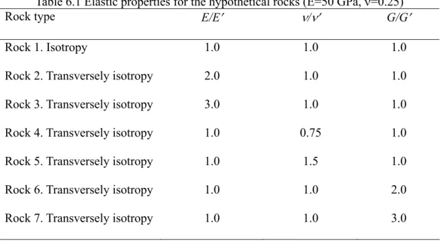
... 13 Table 6.1 Elastic properties for the hypothetical rocks (E=50 GPa, ν=0.25)... 101

LIST OF FIGURES

Fig. 1.1 Structure of the thesis... 4

Fig. 3.1 ( Px, Py, Pz ) acting in an inclined transversely isotropic full-space... 18

Fig. 4.1 Separate the full-space into three imaginary regions of −∞<z<0−, + − _{< <0} 0 z and ₀+ <_z<+∞_{... 47}

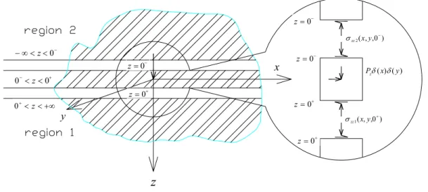
Fig. 4.2 A closed contour on the upper γ-plane. ... 55

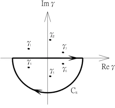
Fig. 4.3 A closed contour on the lower γ-plane. ... 56

Fig. 4.4 Spherical co-ordinate system (k, θx)... 61

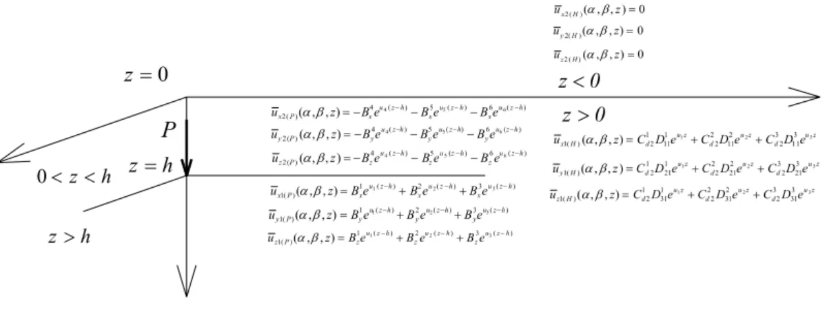
Fig. 5.1 Displacement function for point loads (Px, Py, Pz) acting at (0, 0, h) of a half-space... 72

Fig. 5.2 Separate the half-space into two imaginary region of 0 z< <0+ and +∞ < < + _z 0 . ... 76

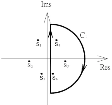
Fig. 5.3 A closed contour on right-hand side of s-plane... 84

Fig. 5.4. A closed contour on left-hand side of s-plane. ... 85

Fig. 6.1 Spherical co-ordinate system (r, ϕ, ξ)... 99

Fig. 6.2.(a) At the position x=y=z=1, the effect of φ on the normalized displacement ux*r/Pz... 107

Fig. 6.2.(b) At the position x=y=z=1, the effect of φ on the normalized displacement uy*r/Pz... 108

Fig. 6.2.(c) At the position x=y=z=1, the effect of φ on the normalized displacement uz*r/Pz... 109

Fig. 6.3.(a) At the position x=y=z=1, the effect of φ on the non-dimensional normal stress σxx*r2/Pz...110

Fig. 6.3.(b) At the position x=y=z=1, the effect of φ on the non-dimensional normal stress σyy*r2/Pz...111

Fig. 6.3.(c) At the position x=y=z=1, the effect of φ on the non-dimensional normal stress σzz*r2/Pz...112

Fig. 6.3.(d) At the position x=y=z=1, the effect of φ on the non-dimensional shear stress τyz*r2/Pz...113

Fig. 6.3.(e) At the position x=y=z=1, the effect of φ on the non-dimensional shear stress τzx*r2/Pz...114

Fig. 6.3.(f) At the position x=y=z=1, the effect of φ on the non-dimensional shear stress τxy*r2/Pz...115

Fig. 6.4.(a) At the position φ=90°, ξ=45°, the effect of ϕ on the non-dimensional normal stress σxx*r2/Pz...116

Fig. 6.4.(b) At the position φ=90°, ξ=45°, the effect of ϕ on non-dimensional normal stress σyy*r2/Pz...117

Fig. 6.4.(c) At the position φ=90°, ξ=45°, the effect of ϕ on the non-dimensional normal stress σzz*r2/Pz...118

Fig. 6.4.(d) At the position φ=90°, ξ=45°, the effect of ϕ on the non-dimensional shear stress τyz*r2/Pz...119

Fig. 6.4.(e) At the position φ=90°, ξ=45°, the effect of ϕ on the non-dimensional shear stress τzx*r2/Pz... 120 Fig. 6.4.(f) At the position φ=90°, ξ=45°, the effect of ϕ on the non-dimensional

shear stress τxy*r2/Pz... 121

Fig. 6.5 Effect of ratios of E/E'_, υ/υ' _{and G/G}'

on normalized vertical

displacement ... 124 Fig. 6.6 Effect of ratios of E/E'_, υ/υ' _{and G/G}'

on non-dimensional lateral displacement ... 125

LIST OF SYMBOLS

ENGLISH SYMBOLS ) 6 ~ 1 (i=

a_i elasticity constants defined in Eq.(3.04) ) 6 ~ 1 , (i j=

a_ij elasticity constants defined in Appendix A 3

2 1,A ,A

A functions of elasticity constants defined in

Eqs.(3.48a)-(3.48c) i z i y i x A A

A , , undetermined coefficients defined in Eqs.(3.49a)-(3.49c)

) 6 1 ( , , , , , − = i i z2 i y2 i x2 i z1 i y1 i x1 A A A A A A

undetermined coefficients defined in Eqs.(3.52a)-(3.52b)

C_{i j}( ,i j= 1 6~ ) elastic moduli or elasticity constants defined in Eq.(3.04)

) 3 ~ 1 , ( j i j=

D_i the cofactors of the third-order determinant det[d_ij] )

3 1 , (

dij i j = ～ coefficients defined in Eqs.(3.46a)-(3.46f)

E, _E'_{, υ, υ}'_{, G}' _{elastic constants of a transversely isotropic medium}

i complex number (= − 1)

ij

l direction cosines defined in Eq.(3.05)

P_x, P_y, P_z point loads in a Cartesian co-ordinate system

r radius of a circle

r, θ, z a cylindrical co-ordinate system

z y

x F F

F, , body force components in a Cartesian co-ordinate system

6 5 4 3 2 1,u ,u ,u ,u ,u

u roots of the characteristic equation

) , , (x y z ui displacement components ) , , ( z

u_i α β Double Fourier transforms of u_i(x,y,z) ) , , (α β γ i U Fourier transforms of Ui(α,β,z) ) , , ( s U_i α β Laplace transforms of U_i(α,β,z) x, y, z a Cartesian co-ordinate system

GREEK SYMBOLS

γ β

α , , integers used in Fourier transform

δ( ) Dirac delta function

z , , _{yy z}

xx ε ε

ε normal strain components in a Cartesian co-ordinate

system (x,y,z) z' ' ' ' ' 'x, yy, z x ε ε

ε normal strain components in a Cartesian co-ordinate

system (x',y',z') xy

z, ,γ γ

γ_{xz y} shear strain components in a Cartesian co-ordinate system

) , , (x y z y' x' z' ' ' ' ,γ ,γ

γxz y shear strain components in a Cartesian co-ordinate system

) ' , ' , ' (x y z z z , ,σ σ

σxx yy normal stress components in a Cartesian co-ordinate

z' z' ' ' ' ' ,σ ,σ

σxx yy normal stress components in a Cartesian co-ordinate

system (x',y',z') ) , , ( , ) , , ( ), , , ( z z z zz yy xx β α σ β α σ β α σ

Double Fourier transforms of normal stresses

) , , ( , ) , , ( ), , , ( z z z yz xz xy β α τ β α τ β α τ

Double Fourier transforms of shear stresses

z x z, ,τ τ

τ_{xy y} shear stress components in a Cartesian co-ordinate system

) , , (x y z z' x' z' ' ' ' ,τ ,τ

τ_{xy y} shear stress components in a Cartesian co-ordinate system

) ' , ' , ' (x y z

φ the rotation of the transversely isotropic planes

ω angular frequency

CHAPTER I

INTRODUCTION

The failure of a foundation in soil/rock is often caused by extra strains (deformations) or stresses. This fact is particularly important when structures impose very large loads on the underlying soil/rock. Normally, however, the magnitude and distribution of strains and stresses in soil/rock are predicted using numerical/analytical solutions that model the constituent materials as a linearly elastic, homogeneous and isotropic continuum. These solutions can not count the anisotropy of soils/rocks that are deposited via sedimentation over a long period of time, or rock masses cut by regular discontinuities, such as cleavages, foliations, stratifications, schistosities, and joints. Anisotropic soils/rocks are commonly modeled as transversely isotropic (cross-anisotropic) materials based on the practical engineering considerations. Nevertheless, the effects of inclination of discontinuities on the displacements and stresses are of interest. Hence, this thesis derives the analytical solutions for displacements and stresses due to three-dimensional point loads in a transversely isotropic medium with inclined planes of elastic symmetry.

Briefly, this thesis aims to derive the three-dimensional elastic solutions in a transversely isotropic full space and a half space subject to a three-dimensional point load. Employing the Fourier transform, the governing partial differential equations can be simplified as an ordinary differential equation. Then, three distinct approaches were used to solve the ODE for both infinite and semi-infinite solids in this thesis. The solutions show that there are identical for different approaches. The major deriving

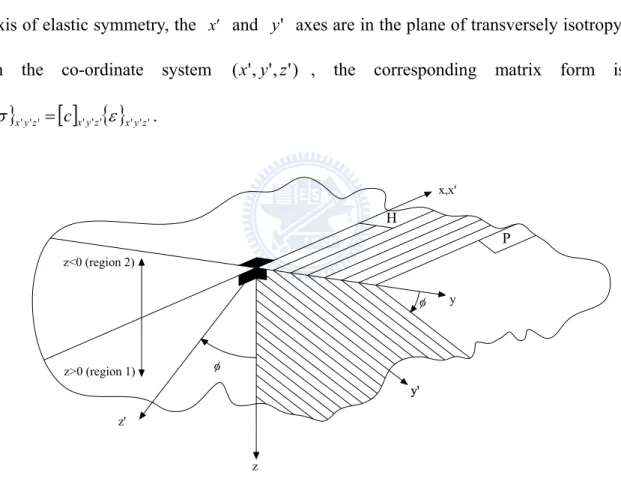
procedures are shown in Fig. 1.1. The three approaches are briefly described as follows: Firstly, we solve the nonhomogeneous ordinary differential equations by the methods of undetermined coefficients and separate variables, and obtain the homogeneous and particular solution for both a full-space and a half-space. Secondly, we separate the full-space into three regions of −∞<z<0− (region 2-upper half space) , 0− <z<0+ (imaginary space) and ₀+ <_z<+∞ _{(region 1-lower half space) or the half-space into} two regions of _{0 z< <0}+ _{(imaginary space) and 0}+ _{< z<+∞ (region 1), the point} load force is loading in the region of ₀− _{< z<0}+ _{for full-space and 0 z< <0}+ _for half-space. The right-hand side of the governing equations are zero in regions of

− < < ∞

− z 0 or ₀+ <_z<+∞_{, the equations are said to be homogeneous. Hence, we} can solve the boundary-value problem consisting of the three or two regions for full-space or half-space. Thirdly, the Fourier transform respect to variables of z can reduce the aforementioned ordinary differential equations to algebraic equations. This method, which include three times of Fourier transform respect to variables of x, y and z, is also called Triple Fourier transform method. In the other word, the triple Fourier transforms with respect to x, y, and z could reduce the full-space problem of solving partial differential equations to algebraic equations. However, in the half-space, the double Fourier transforms with respect to x, and y can reduce the problem of solving partial differential equations to ordinary differential equations. Furthermore, by collocating the Laplace transform can reduce the aforementioned ordinary differential equations to algebraic equations. Hence, the displacement components in the triple Fourier transformed domains (U_i(α,β,γ)), or in the double Fourier and Laplace ones (U_i(α,β,s)) can be obtained.

Finally, the present fundamental solutions are derived by performing the required triple inverse Fourier transforms, or double inverse Fourier and Laplace transforms. These transformations are powerful to generate the displacements and stresses resulting from the three-dimensional point loads, acting in an inclined transversely isotropic material.

The content of this thesis, includes that Chapter Ⅱ provides a general literature review on the existing relevant solutions for the transversely isotropic media; Chapter Ⅲ introduction the basic theory of Fourier and Laplace integral transforms in a Cartesian co-ordinate system; Chapter Ⅳ and Ⅴ present the detailed derivations for three dimensional elastic solutions of an anisotropic full-space and half-space subjected to point loads by employing the Fourier and Laplace integral transforms, respectively. A series of parametric study using the present analytical solutions for displacements or stresses is conducted by four illustrative examples; The numerical results are demonstrated in Chapter Ⅵ ; Eventually, Chapter Ⅶ includes summary and recommendations for future work.

PDE in x,y,z domains

Double Fourier Transform with respect to variable of x and y

ODE in α,β,z domain

Traditional Method Imaginary space

method

Algebraic equations method

General solutions in full-space or half-space problem knowing

boundary conditions Solving of ūi(α,β,z) Solving of ui (x,y,z) Fourier Transform variable z to γin full-space Laplace Transform variable z to s in half-space Solution of algebraic equations Ūi(α,β,γ) Inverse Laplace Transform with respect to variable of s Inverse Fourier Transform with respect to variable of γ

Inverse Double Fourier Transform

with respect to variable of α,β

Solution of algebraic equations

Ūi(α,β,s)

Fig. 1.1 Structure of the thesis

CHAPTER II

LITERATURE REVIEW

The elasticity of transversely isotropic materials is an important field of applied mechanics and engineering science. With the rapid development of modern technologies, the theory of elasticity has become increasingly significant. In addition, the field with which the theory has been typically associated, such as civil engineering and material engineering, also, many emerging technologies demand the development of transversely isotropic elasticity. Some immediate examples are piezo-film technology, anisotropic piezo-electric technology, functionally gradient materials (FGMs), and those involving transversely isotropic and layered microstructures, such as multi-layer systems and tribology mechanics of magnetic recording devices (Pan and Yuan, 2000).

The mathematical details of the basic equations of elasticity can be found in a variety of textbooks (e.g., Sneddon (1951) and Lekhnitskii (1981)). The basic equations of elasticity are geometric equations, constitutive equations, and equations of equilibrium. In tensor form, the geometric equations of strain-displacement relation in a Cartesian co-ordinate system can be written as:

) ( 2 1 , ,j ji i ij = u +u ε (2.1) The constitutive equations of stress-strain relation in linear elasticity are represented

as:

kl ijkl

ij c ε

Considering the static state, the equations of motion can be reduced to the equations of equilibrium as follows: 0 ,j+ i = ij F σ (2.3) Eqs. (2.1)-(2.3) will be further discussed in Chapter 3.1.

There are six basic equations of Eq. (2.1), six equations of Eq. (2.2), and three equations of Eq. (2.3). Hence, total fifteen equations of Eqs. (2.1)-(2.3) contain fifteen unknows of three groups of u , _i σ_ij, and ε_ij. Generally, it is unrealistic to solve the fifteen unknows all together. We often take one group of unknows or some unknows from different groups as the basic variables. The displacements of u are frequently _i adopted as the basic variables to be found. In such a method, the other unknows of two groups of σ_ij and ε_ij must be eliminated from the equations. More details

about the uniqueness and possibility of other similar displacement presentations can be found in the works by Zou et al. (1994) and Ding et al. (1996). However, if we take the stress components (σ_ij) as the basic unknowns, these variables should be satisified

with corresponding stress boundary conditions and the compatibility conditions between displacements and strains. Then, the solutions for stresses, and coresponding strains and displacements, can be derived. In anisotropic elasticity, the stress method is usually adopted to solve some relatively simpler problems (Ding et al., 2006). A summary of the earlier works in this respect can be found in the monograph of Lekhnitskii (1981). Base on the stress method, the general solutions of axisymmetric problems of transversely isotropic media were derived by Ding (1987), Wang and Wang (1989). In many other cases, it may be easier to find some stresses and some

displacements but not all the variables of one single group. The state-space method usually deals with Eqs. (2.1)-(2.3) with two groups of unknowns. It has been utilized to solve the elasticity problems by Tarn (2002) and Georgiadis et al. (1999).

The equilibrium equations of Eq. (2.3) for infinite or semi-infinite solids are partial differential equations. Partial differential equations arise in connection with various physical and geometrical problems when the functions involved depending on two or more independent variables. It is fair to say that only the simplest physical systems can be modeled by ordinary differential equations. For infinite or semi-infinite domains, the method of integral techniques is applicable for the partial differential equations to reduce them to ordinary differential equations or algebraic equations. The integral techniques include the Fourier, Laplace, Hankel, and Mellin transforms are often employed to achieve the goal.

Pan and Yuan (2000) obtained the analytical solutions for stresses and strains in anisotropic bimaterials by double Fourier integral transforms. Liao and Wang (1998) presented the solutions of displacements and stresses in a transversely isotropic half-space by using Hankel and finite Fourier exponential transforms. Nevertheless, in transient dynamic problems, Laplace transforms are the most useful tools to transform the variable of time. To the best of the author′s knowledge, no solutions for displacements and stresses have been proposed by employing the Laplace transforms with respect to the spatial co-ordinate (x, y, or z) in a Cartesian co-ordinate system. the Laplace transforms are adopted for solving the half space problem in this thesis.

This chapter reviews the current steate of knowledge with respect to the point loading problem of a transversely isotropic medium. Existing analytical three-dimensional

solutions of displacement or stresses subjected to a point load in infinite or semi-infinite space for a transversely isotropic medium are summerized.

2.1 Three-Dimensional Elastic Solution for Displacements and Stresses in a Transversely Isotropic Full Space

Solutions to the problem of a point load acting in the interior of a full-space are called the fundamental solutions or the elastic Green’s function solutions (Pan et al., 1976 and Tarn et al., 1987). In the problems of infinite media, Willis (1965) estimated the elastic interaction energy of two infinitesimal dislocation loops in transversely isotropic magnesium and zinc media. There were two reasons to choice this medium, the first being the case of presentation of the results afforded by the axial symmetry, facilitating a ready comparison with the isotropic results. The second one was that to find the closed-form expressions for fundamental elasticity tensor for such a medium were possible.

Ting and Lee (1996) obtained the solution of Green’s function for three-dimensional space of general anisotropic inclined medium subjected to a unit point force. It was expressed in terms of the Stroh eigenvalues pv (v=1, 2, 3) on the inclined plane, and it

remained valid for the degenerate cases when p1=p2, and p1=p2=p3. The Stroh

eigenvalues pv were the roots with positive imaginary part of a sextic algebraic equation.

The Green’s function was simple when the sextic equation was a cubic equation in p2. This was the case for any point in a transversely isotropic material and for points on a symmetric plane of cubic, and monoclinic materials.

mechanics and in particular numerical formulations of boundary element methods. Many investigators have presented analytical solutions for displacement under a point load in a transversely isotropic full-space, whose the transversely isotropic planes are parallel to the horizontal loading surface. A summary of the existing solutions is given in Table 2.1.

Table 2.1 Existing solutions for a transversely isotropic full-space subjected to a point load

Author Analytical methods Type of loading Presented solutions Chowdhury (1987) methods of images and

Hankel transforms

vertical all displacements

Pan (1989) vector functions 3D all displacements Willis (1965) Fourier transforms vertical all displacements Elliott (1948) potential functions vertical all displacements Chen (1966) potential functions vertical

horizontal

all displacements all displacements Pan and Chou (1976) potential functions 3D all displacements Fabrikant (1989) potential functions 3D all displacements Sveklo (1969) complex variables vertical all displacements Tarn and Wang (1987) Fourier and Hankel

transforms

3D all displacements

Lu (1991) Fourier and Hankel transforms

3D all displacements

Liao and Wang (1998) Fourier and Hankel transforms

Sheu (2004) Fourier and Hankel transforms

3D all displacements

Table I indicates the analytical methods, the type of loading and the presented results. To the best of the authors’ knowledge, no closed-form solutions for the displacement have been obtained in cases in which the planes of transverse isotropy inclines to the full-space subjected to 3D point loads (Px, Py, Pz), as displayed in Figure 3.1. In this thesis, the methods proposed by Willis (1965) for a transversely isotropic medium are followed. That is, the triple Fourier transforms are adopted to obtain the integral expressions of Green’s displacement; then, the triple inverse Fourier transforms and residue calculus are performed to integrate the contours. However, Willis’s expressions for Green’s function are only valid when the elastic constants fulfill conditions that enable inverse transforms to be carried out (Tarn et al., 1987). Notably, the main difference between Willis’s approach (1965) and that proposed herein was the use of orthogonal vectors. In the former, two axes were on the transversely isotropic plane, and the third was parallel to the axis of rotation associated with elastic symmetry. Accordingly, a state of plane strain was assumed in that procedure.

2.2 Three-Dimensional Elastic Solution for Displacements and Stresses in a Transversely Isotropic Half Space

A point load solution is the basis of complex loading problems. For an isotropic solid, it has been studied by Kelvin (Thompson, 1848) for a full-space, Boussinesq

(1885) and Cerruti (1888) for a half-space with a vertical and horizontal point load, respectively. In the case of a single concentrated force acting in the interior of a half-space, Mindlin (1936) proposed closed-form solutions for an isotropic medium using the principle of superposition of eighteen nuclei. Mindlin derived analytical solutions following the Kelvin's (1848) approach and satisfying the condition of vanishing traction on a plane boundary. However, the calculation of nuclei for a half-space is very difficult (Mindlin and Cheng, 1950). Dean et al. (1944) recommended another approach for the same problem by the method of images. Some of their solutions can be extended to anisotropic media, whereas others are difficult. For the displacements and stresses in transversely isotropic media subjected to a point load, analytical solutions have been presented by several investigators. Some of the solutions were directly derived using the approaches for isotropic solutions (Michell, 1900; Wolf, 1935; Koning, 1957; Barden, 1963; de Urena et al., 1966; Misra and Sen, 1975; Chowdhury, 1987; Pan, 1989). Nevertheless, others employed complex mathematics techniques, such as Fourier transformations (Kröner, 1953; Willis, 1965; Lee, 1979), potential functions (Lekhnitskii, 1940; Elliott, 1948; Shield, 1951; Eubanks and Sternberg, 1954; Lodge, 1955; Hata, 1956; Chen, 1966; Pan and Chou, 1976; Pan and Chou, 1979; Okumura and Dohba, 1989; Fabrikant, 1989; Lin et al., 1991; Hanson and Wang, 1997) and complex variables (Sveklo, 1964, 1969), etc. The summary of the existing solutions is given in Table 2.1. Table 2.1 indicates the type of analytical space, the load, and the results presented in their solutions. Because of mathematical difficulty or oversimplification for solving the problems, these solutions were limited to three-dimensional problems with partial results of displacements (Michell, 1900; Shield,

1951; Barden, 1963) and stresses (Michell, 1900; Shield, 1951; Barden, 1963; Misra and Sen, 1975; Pan and Chou, 1979; Chowdhury, 1987; Fabrikant, 1989), or axially symmetric problems invariant with the tangential co-ordinate, θ (Lekhnitskii, 1940; Elliott, 1948; Koning, 1957; Sveklo, 1964; de Urena et al., 1966; Misra and Sen, 1975). Neglecting the θ, the solutions cannot be extended to solve a half-space problem subjected to asymmetric loads. Pan and Chou (1979) proposed a more general solution using potential functions. In their solution, the buried loads can be vertical or horizontal with respect to the boundary plane. However, only the stress components related to the z-direction were given (i.e., σzz, σzx, σzy), and the expressions for the solution are quite lengthy.

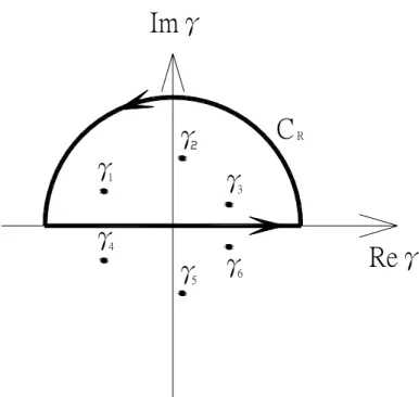
Table 2.2 Existing solutions for transversely isotropic media subjected to a point load Author Space Type of loading Solutions

Michell (1900) half vertical vertical surface displacement, and partial stresses

(inapplicable to boundary value problems) Wolf (1935) half vertical all displacements and stresses

(oversimplified the elastic constants) Koning (1957) half vertical all displacements and stresses Barden (1963) half vertical vertical surface displacement,

and stresses on load axis de Urena et al.

(1966)

half vertical all displacements and stresses Misra and Sen

(1975)

half vertical all displacements, and stresses on load axis (oversimplified the elastic constants) Chowdhury (1987) full

half

vertical buried, vertical

all displacements, and stresses on load axis all displacements, and stresses on load axis Pan (1989) full 3-D all displacements and stresses Kröner (1953) half vertical all displacements (dimensionally incorrect)

Willis (1965) full vertical all displacements (cumbersome and inaccurate) Lee (1979) half buried, vertical all stresses (complicated)

Lekhnitskii (1940) half vertical all stresses (incomplete)

Elliott (1948) full vertical all displacements and stresses (incomplete) Shield (1951) half buried, vertical all displacements and stresses at the surface

Eubanks and Sternberg (1954)

half vertical (completeness of Lekhnitskii’s method) Lodge (1955) (transformed anisotropic problem

into isotropic one, inapplicable to general boundary value problems) Hata (1956) half vertical (rederived the Elliott’s and Lodge’s solution) Chen (1966) full vertical

horizontal

all displacements and stresses all displacements Pan and Chou

(1976)

Table 2.2. Existing solutions for transversely isotropic media subjected to a point load (continued)

Author Space Type of loading Solutions Pan and Chou

(1979)

half buried, vertical buried, horizontal

all displacements, and stresses on load axis all displacements, and partial stresses (potential functions assumed are lengthy) Okumura and

Dohba (1989)

half vertical all displacements Fabrikant (1989) full

half

3-D 3-D

all displacements, and partial stresses all displacements, and partial stresses (solution of the shear stress is wrong) Lin et al. (1991) half vertical, horizontal all displacements and stresses Hanson and Wang

(1997)

half buried, 3-D (only the potential functions listed)

Sveklo (1964) half vertical all displacements Sveklo (1969) full half vertical buried, vertical all displacements all displacements

Following the method proposed by Tarn and Wang (1987), Lu (1991) presented analytical solutions for the displacements in a full or half soil space (transverse isotropy) under a long-term consolidation. However, a part of the solutions might be error in handwriting. Utilizing the approaches proposed by Lu (1991), closed-form solutions for displacements and stresses in a transversely isotropic half-space subjected to a point load are rederived and parts of the results are published (Liao and Wang, 1998). However, the solutions are limited to the cases of planes of transverse isotropy parallel to the horizontal loading surface.

The solution of the stresses and displscements in a half-space or a layered solid with transverse isotropy is fundamental to the development of the theory of elasticity and is of importance to many engineering applications. Ding (1987) presented a

unified solution for a point force applied on the surface/in the interior of a half-space. The solution could be extended to the problem of layered media using the state-space and Fourier transform methods. Hence, to solve the problems of semi-infinite media, Ding considered a transversely isotropic medium in a Cartesian co-ordinate system (x, y, z), whose z-axis is perpendicular to the isotropic plane of material. Any point force (or concentrated force) applied in the body can be resolved into three components T, Q and P in x-, y-, and z-direction, respectively. Ding assumed that an arbitrary point force was applied at the origin. It can be decomposed the problem into three sub-problems by using the principle of superposition; namely, the solution corresponding to a vertical force, P, in the positive z-direction, the solution to a tangential force, Tx=T, in the x-direction, as well as the solution to a tangential force,

Ty=Q, in the y-direction. The last solution can be obtained from the second solution by

a co-ordinate transform with x replaced by y, and y by –x, respectively. However, it is clear that Ding’s solutin has not yielded the analytical solutions of displacements and stresses for an inclined transversely isotropic material owing to three–dimensional point loads. All the fundamental solutions of literature for transversely isotropic materials being the case of axisymmetric problem.

CHAPTER Ⅲ

BASIC THEORY

To derive the solutions for stresses, strains, and displacements in finite domains with simple geometry, the method of separation of variables is usually applicable for the partial differential equations to reduce to the ordinary differential equations (Chiang, 1997). Then the solutions can be constructed by superposition of eigenfunctions. However, considering the domain is infinite or semi-infinite, it is hard to achieve a similar reduction. Thus, the integral techniques include the Fourier, Laplace, Hankel, and Mellin transforms are often utilized to attain the goal. Among them, the Fourier and Laplace transforms are basic and most useful. Generally, the governing equations for infinite or semi-infinite solids are partial differential equations. The Fourier and Laplace integral transforms are efficient methods for solving the partial differential equations and corresponding boundary value problems. Employing the two methods can reduce the problem from solving partial differential equations to ordinary differential equations or algebraic equations.

3.1 Basic Equations for Elastic Boundary Value Problems Constitutive equations and transformation of elastic constants

The constitutive equations in linear elasticity are represented by the generalized Hooke′s law. If the state of vanishing strain corresponds to zero stress, then in Cartesian co-ordinates, the generalized Hooke′s law can be written as:

kl ijkl

ij c ε

where c are components of a fourth-rank tensor, repressenting the properties of a _ijkl material, which generally varies from one point to another in the material. The c _ijkl are called elastic stiffness constants. Since Eq. (3.01) contains nine equations (corresponding to all possible combinations of the subscripts i and j and each equation contains nine strain variables), there are 81 elastic stiffness constants. These are not all independent hower. It will be seen that c_ijkl =c_jikl =c_ijlk =c_jilk, which reduces the number of independent constants to 36. In addition, the c_ijkl =c_klij, and this means the constants are further reduced to 21. This is the maxium number of constants for any medium.

In a Cartesian co-ordinate system, (x,'y,'z'), the Eq. (3.01) can then be expressed as: ⎥ ⎥ ⎥ ⎥ ⎥ ⎥ ⎥ ⎥ ⎦ ⎤ ⎢ ⎢ ⎢ ⎢ ⎢ ⎢ ⎢ ⎢ ⎣ ⎡ ⎥ ⎥ ⎥ ⎥ ⎥ ⎥ ⎥ ⎥ ⎦ ⎤ ⎢ ⎢ ⎢ ⎢ ⎢ ⎢ ⎢ ⎢ ⎣ ⎡ = ⎥ ⎥ ⎥ ⎥ ⎥ ⎥ ⎥ ⎥ ⎦ ⎤ ⎢ ⎢ ⎢ ⎢ ⎢ ⎢ ⎢ ⎢ ⎣ ⎡ ' ' ' ' ' ' ' ' ' ' ' ' 66 65 64 63 62 61 56 55 54 53 52 51 46 45 44 43 42 41 36 35 34 33 32 31 26 25 24 23 22 21 16 15 14 13 12 11 ' ' ' ' ' ' ' ' ' ' ' ' y x x z z y z z y y x x y x x z z y z z y y x x C C C C C C C C C C C C C C C C C C C C C C C C C C C C C C C C C C C C γ γ γ ε ε ε τ τ τ σ σ σ (3.02)

The number of elastic constants c for describing their deformability is 21, 9, 5, _ijkl and 2 for generally anisotropic, orthotropic, transversely isotropic, and isotropic material, respectively. Thus, for a general anisotropic elastic material, there are 21 independent elastic stiffness constants. If there exist three orthogonal planes of elastic symmetry at any point in a solid, then there are 9 independent elastic stiffness constants, and the material is said to be orthotropic. If at any point there is an axis of symmetry

such that the elastic properties in any direction within a plane perpendicular to the axis are all the same, the number of independent elastic stiffness constants will reduce to 5. The plane is called an isotropic plane and the material is called a transversely isotropic material. If any plane in the material is a plane of elastic symmetry, then the material is isotropic, and has only 2 independent elastic stiffness constants.

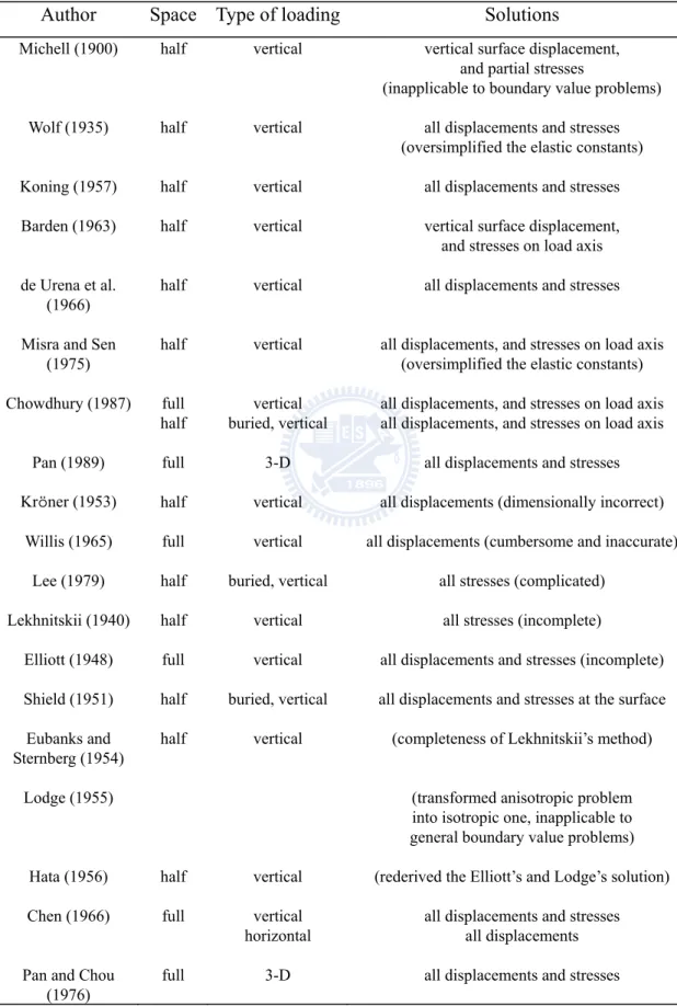
Fig. 3.1 displays a transversely isotropic medium, in which the 'z axis is the rotation axis of elastic symmetry, the x' and 'y axes are in the plane of transversely isotropy. In the co-ordinate system (x,'y,'z') , the corresponding matrix form is

{ }

σ x'y'z' =

[ ]

c x'y'z'

{ }

ε x_'y_'z_'. z<0 (region 2) z>0 (region 1) H P x,x' φ φ y' y' z' z y

Fig. 3.1 ( Px, Py, Pz ) acting in an inclined transversely isotropic full-space

Regarding the different co-ordinate system (x,y,z), the constitutive equations will have the same form as

{ }

σ _xyz =

[ ]

a _xyz

{ }

ε _xyz. Hence, the generalized Hooke′s law for the transversely isotropic material can be expressed as:

⎥ ⎥ ⎥ ⎥ ⎥ ⎥ ⎥ ⎥ ⎦ ⎤ ⎢ ⎢ ⎢ ⎢ ⎢ ⎢ ⎢ ⎢ ⎣ ⎡ ⎥ ⎥ ⎥ ⎥ ⎥ ⎥ ⎥ ⎥ ⎦ ⎤ ⎢ ⎢ ⎢ ⎢ ⎢ ⎢ ⎢ ⎢ ⎣ ⎡ − − − − − − = ⎥ ⎥ ⎥ ⎥ ⎥ ⎥ ⎥ ⎥ ⎦ ⎤ ⎢ ⎢ ⎢ ⎢ ⎢ ⎢ ⎢ ⎢ ⎣ ⎡ ⎥ ⎥ ⎥ ⎥ ⎥ ⎥ ⎥ ⎥ ⎦ ⎤ ⎢ ⎢ ⎢ ⎢ ⎢ ⎢ ⎢ ⎢ ⎣ ⎡ = ⎥ ⎥ ⎥ ⎥ ⎥ ⎥ ⎥ ⎥ ⎦ ⎤ ⎢ ⎢ ⎢ ⎢ ⎢ ⎢ ⎢ ⎢ ⎣ ⎡ ' ' ' ' ' ' ' ' ' ' ' ' 4 5 5 2 5 3 5 3 5 3 1 4 1 5 3 4 1 1 ' ' ' ' ' ' ' ' ' ' ' ' 66 44 44 33 13 13 13 11 12 13 12 11 ' ' ' ' ' ' ' ' ' ' ' ' 0 0 0 0 0 0 0 0 0 0 0 0 0 0 0 0 0 0 0 0 0 2 0 0 0 2 0 0 0 0 0 0 0 0 0 0 0 0 0 0 0 0 0 0 0 0 0 0 0 0 y x x z z y z z y y x x y x x z z y z z y y x x y x x z z y z z y y x x a a a a a a a a a a a a a a a a a a C C C C C C C C C C C C γ γ γ ε ε ε γ γ γ ε ε ε τ τ τ σ σ σ (3.03)

where σ_x'x', σ_y'y', σ_z'z' are normal stresses; ε_x'x', ε_y'y', ε_z'z' are normal strains;

' z ' y

τ , τz'x', τx'y' are shear stresses; γy'z', γz'x', γx'y' are shear strains, and C11,

12

C , C13 , C33 , C44 , C66 are elastic moduli or constants. Since

66 11 12 C 2C

C = − , hence, only C11, C13, C33, C44, C66 are independent for a

transversely isotropic material. The relationship between C11, C13, C33, C44,

66

C and a1, a2, a3, a4, a5 can be presented in terms of five elastic constants as:

) E E 2 1 )( 1 ( ) E E 1 ( E C a 2 ' ' 2 ' ' 11 1 υ υ υ υ − − + − = = , 2 ' ' ' 33 2 E E 2 1 ) 1 ( E C a υ υ υ − − − = = , ' 44 5 C G a = = , 44 2 ' ' ' 44 13 3 C E E 2 1 E C C a + − − = + = υ υ υ , ) 1 ( 2 E 2 C C C a_{4 66} 11 12 υ + = − = = (3.04) where:

1. E and 'E are Young′s moduli in the plane of transverse isotropy and in a direction normal to it, respectively.

2. υ and υ are Poisson′s ratios characterizing the lateral strain response in the plane '

of transverse isotropy to a stress acting parallel or normal to it, respectively. 3. G' is the shear modulus in planes normal to the plane of transverse isotropy.

If a new co-ordinate system (x, y, z) is obtained from the original system (x', y',

'z) by rotation through an angle φ about the common axis x=x' (the axis of x and

'

x parallel to the strike of transverse plane). The matrix of direction cosines lij for the

transformation formulae of the elastic constants are:

[ ]

⎥ ⎥ ⎥ ⎦ ⎤ ⎢ ⎢ ⎢ ⎣ ⎡ − = ⎥ ⎥ ⎥ ⎦ ⎤ ⎢ ⎢ ⎢ ⎣ ⎡ = φ φ φ φ cos sin 0 sin cos 0 0 0 1 l l l l l l l l l l 33 32 31 23 22 21 13 12 11 ij (3.05) where i, j=1-3.

The elastic stiffnesses matrix in the old co-ordinate system (x,'y,'z') is

[ ]

c _{x' zy''} . Therefore, the elastic stiffnesses matrix

[ ]

a xyz in the new co-ordinate system (x,y,z)

can be expressed as:

[ ]

[ ]

[ ]

[ ]

⎥ ⎥ ⎥ ⎥ ⎥ ⎥ ⎥ ⎥ ⎦ ⎤ ⎢ ⎢ ⎢ ⎢ ⎢ ⎢ ⎢ ⎢ ⎣ ⎡ = = 66 65 64 63 62 61 56 55 54 53 52 51 46 45 44 43 42 41 36 35 34 33 32 31 26 25 24 23 22 21 16 15 14 13 12 11 ' ' ' a a a a a a a a a a a a a a a a a a a a a a a a a a a a a a a a a a a a q c q a _{xyz ij} T _ij z y x (3.06)

[ ]

⎥ ⎥ ⎥ ⎥ ⎥ ⎥ ⎥ ⎥ ⎦ ⎤ ⎢ ⎢ ⎢ ⎢ ⎢ ⎢ ⎢ ⎢ ⎣ ⎡ + + + + + + + + + = 21 12 22 11 23 11 21 13 23 12 22 13 23 13 22 12 11 21 11 32 12 31 13 31 11 33 13 32 12 33 13 33 12 32 11 31 21 32 22 31 23 31 21 33 23 32 22 33 23 33 22 32 21 31 31 32 31 33 32 33 2 33 2 32 2 31 21 22 21 23 22 23 2 23 2 22 2 21 11 12 11 13 13 12 2 13 2 12 2 11 ij l l l l l l l l l l l l l l 2 l l 2 l l 2 l l l l l l l l l l l l l l 2 l l 2 l l 2 l l l l l l l l l l l l l l 2 l l 2 l l 2 l l l l l l l l l l l l l l l l l l l l l l l l l l l q (3.07) where i, j=1-3.

The new elastic constants of

[ ]

a _xyz obtained directly from the old elastic conctant a1-a5 and φ. It is important to note that

[ ]

a _xyz exist 13 elastic constants under the

plane of elastic symmetry system, and the expressions of the elastic constants aij(i,

j=1-6) with respect to a1-a5 and φ are presented in Appendix A. Appendix A show that

the new constants of a₁₅ = a₁₆ =0 , a₂₅ = a₂₆ =0 , a₃₅ = a₃₆ =0 , a₄₅ = a₄₆ =0 ,

0 54 53 52 51 =a =a =a = a and a₆₁=a₆₂ =a₆₃ =a₆₄ =0

Then, the generalized Hooke′s law for a transversely isotropic material is:

{ }

σ xyz =

[ ]

a xyz

{ }

ε xyz (3.08)

where

{ }

σ _xyz and

{ }

ε _xyz are vectors of stress and engineering strain, respectively. In Cartesian co-ordinates, they are

{ }

[

]

T xy zx yz zz yy xx xyz σ σ σ τ τ τ σ = (3.09)

{ }

[

]

T xy zx yz zz yy xx xyz ε ε ε γ γ γ ε = . (3.10) Strain-displacement relations

When a sign convention for soil and rock problem is required, it is customary to define compressive stresses as positive and tensile stresses as negative. The

strain-displacement relationship under small strain condition in a Cartesian coordinate system is: ⎥ ⎥ ⎥ ⎥ ⎥ ⎥ ⎥ ⎥ ⎥ ⎥ ⎥ ⎥ ⎥ ⎥ ⎦ ⎤ ⎢ ⎢ ⎢ ⎢ ⎢ ⎢ ⎢ ⎢ ⎢ ⎢ ⎢ ⎢ ⎢ ⎢ ⎣ ⎡ ∂ ∂ − ∂ ∂ − ∂ ∂ − ∂ ∂ − ∂ ∂ − ∂ ∂ − ∂ ∂ − ∂ ∂ − ∂ ∂ − = ⎥ ⎥ ⎥ ⎥ ⎥ ⎥ ⎥ ⎥ ⎥ ⎥ ⎥ ⎥ ⎥ ⎥ ⎦ ⎤ ⎢ ⎢ ⎢ ⎢ ⎢ ⎢ ⎢ ⎢ ⎢ ⎢ ⎢ ⎢ ⎢ ⎢ ⎣ ⎡ y u x u x u z u y u z u z uy ux u x y z x z y z y x xy zx yz zz yy xx γ γ γ ε ε ε (3.11)

where ux, uy, and uz are three displacements of a point on the axis of a Cartesian

co-ordinate system.

Generalized Hooke′s law in terms of the derivative of displacements

Hence, from Eqs. (3.08), (3.09), (3.10) and (3.11), the generalized Hooke′s law equations for a transversely isotropic medium in a Cartesian coordinate system can be expressed as: ) ( 14 13 12 11 14 13 12 11 y u z u a z u a y u a x u a a a a a z y z y x yz zz yy xx xx ∂ ∂ + ∂ ∂ − − − − = + + + = ∂ ∂ ∂ ∂ ∂ ∂ γ ε ε ε σ (3.12a) ) ( 24 23 22 12 24 23 22 12 y u z u a z u a y u a x u a a a a a z y z y x yz zz yy xx yy ∂ ∂ + ∂ ∂ − − − − = + + + = ∂ ∂ ∂ ∂ ∂ ∂ γ ε ε ε σ (3.12b)

) ( 34 33 23 13 34 33 23 13 y u z u a z u a y u a x u a a a a a z y z y x yz zz yy xx zz ∂ ∂ + ∂ ∂ − − − − = + + + = ∂ ∂ ∂ ∂ ∂ ∂ γ ε ε ε σ (3.12c) ) ( 44 34 24 14 44 34 24 14 y u z u a z u a y u a x u a a a a a z y z y x yz zz yy xx yz ∂ ∂ + ∂ ∂ − ∂ ∂ − ∂ ∂ − ∂ ∂ − = + + + = ε ε ε γ τ (3.12d) ) ( ) ( ₅₆ 55 56 55 x u y u a x u z u a a a y x z x xy zx zx ∂ ∂ ∂ ∂ γ γ τ + − ∂ ∂ + ∂ ∂ − = + = (3.12e) ) ( ) ( ₆₆ 56 66 56 x u y u a x u z u a a a y x z x xy zx xy ∂ ∂ + ∂ ∂ − + ∂ − = + = ∂ ∂ ∂ γ γ τ (3.12f) Equilibrium equations

In Cartesian coordinates, the equations of motion can be expressed by a tensor form as: i i j ij F ρu&& σ _, + = (i=x, y, z) (3.13)

where ρ is the density of material, F_i is the component of the body force per unit volume in i-direction, and finally the double dot indicates the second order partial differentiation with respect to time t. If the motion of the solid does not involve acceleration, then Eq. (3.13) reduces to the equilibrium equation as:

⎥ ⎥ ⎥ ⎦ ⎤ ⎢ ⎢ ⎢ ⎣ ⎡ = ⎥ ⎥ ⎥ ⎦ ⎤ ⎢ ⎢ ⎢ ⎣ ⎡ + ⎥ ⎥ ⎥ ⎦ ⎤ ⎢ ⎢ ⎢ ⎣ ⎡ ∂ ∂ ∂ ∂ ∂ ∂ ⎥ ⎥ ⎥ ⎦ ⎤ ⎢ ⎢ ⎢ ⎣ ⎡ 0 0 0 / / / z y x zz yz zx yz yy xy zx xy xx F F F z y x σ τ τ τ σ τ τ τ σ (3.14)

where Fx, Fy, and Fz stand for the components of the body forces per unit volume in the

co-ordinate directions, x, y and z, respectively. Substituting Eqs. (3.12a)-(3.12f) (σ_xx,

yy

σ , σ_zz, τ_yz, τ_zx, τ_xy) into Eq. (3.14) enables the equations to be regrouped as Navier-Cauchy equations for an inclined transversely isotropic material as:

x z 2 55 13 z 2 56 14 y 2 56 14 y 2 66 12 x 2 56 2 x 2 55 2 x 2 66 2 x 2 11 F z x u ) a a ( y x u ) a a ( z x u ) a a ( y x u ) a a ( z y u a 2 z u a y u a x u a = + + + + + + + + ∂ ∂ ∂ + ∂ ∂ + ∂ ∂ + ∂ ∂ ∂ ∂ ∂ ∂ ∂ ∂ ∂ ∂ ∂ ∂ ∂ ∂ (3.15a) y z 2 44 23 2 z 2 34 2 z 2 24 2 z 2 56 y 2 24 2 y 2 44 2 y 2 22 2 y 2 66 x 2 56 14 x 2 66 12 F z y u ) a a ( z u a y u a x u a z y u a 2 z u a y u a x u a z x u ) a a ( y x u ) a a ( = ∂ + + + + ∂ ∂ + + + + ∂ ∂ + ∂ + + ∂ ∂ ∂ + ∂ ∂ ∂ ∂ ∂ ∂ ∂ ∂ ∂ ∂ ∂ ∂ ∂ ∂ ∂ (3.15b) z z 2 34 2 z 2 33 2 z 2 44 2 z 2 55 y 2 44 23 2 y 2 34 2 y 2 24 2 y 2 56 x 2 55 13 x 2 56 14 F z y u a 2 z u a y u a x u a z y u ) a a ( z u a y u a x u a z x u ) a a ( y x u ) a a ( = ∂ + + + ∂ ∂ + + + + + ∂ ∂ + ∂ + + ∂ ∂ ∂ + ∂ ∂ ∂ ∂ ∂ ∂ ∂ ∂ ∂ ∂ ∂ ∂ ∂ ∂ ∂ (3.15c) Point loads

For a dynamic elastic problem, an arbitrary time-harmonic body force in z-direction with angular frequency ω can be expressed as (Eringen and Suhubi, 1975; Rahman, 1995): t i *_{( , ,z)e} t) z, y, , ( x F x y ω F_z = _{z (3.16)}

where _F*(_x,_y ,z)

z is the complex amplitude of the body force. Following the

suggestions of Eringen and Suhubi (1975) and Rahman (1995), a concentrated force in z-direction (Fz) can be represented as the form of a body force:

t i e (z) (y) (x)δ δ ω δ z z p F = _(3.17)

where δ ( ) is the Dirac delta function.

Nevertheless, for static problems, the terms associated with time t in Eq. (3.17) should be removed. As this research concerning about the static problems, ω in Eq. (3.17) will be zero. Hence, three-dimensional static point loads with components (Fx,

Fy, Fz) acting at the origin of the co-ordinate can be expressed as the form of body

forces: ) z ( ) y ( ) x ( P F_x = _xδ δ δ (3.18a) ) z ( ) y ( ) x ( P F_y = _yδ δ δ (3.18b) ) z ( ) y ( ) x ( P F_z = _zδ δ δ (3.18c)

Then, the point loads (Fx, Fy, Fz) applied at the point (0, 0, h) of the co-ordinate

system can be described as the form of body forces as: ) ( ) ( ) (x y z h P F_x = _xδ δ δ − (3.19a) ) ( ) ( ) (x y z h P F_y = _yδ δ δ − (3.19b) ) ( ) ( ) (x y z h P F_z = _zδ δ δ − (3.19c)

The Dirac detla function is a mathematical artifice for representing an extremely localized function with a finite total area. For example, δ(x−ξ) is the limit of a spike-like function of x, which is zero almost everywhere expect very near x=ξ. That is, the Dirac detla function has an extremely sharp peak in such a way that its area

above the x axis is unity, i.e., ⎪⎩ ⎪ ⎨ ⎧ ∉ ∈ = −

∫

( ) 1₀ (₍ ,_, ),_), b a if b a if dx x b a _ξ ξ ξ δ (3.20) where (a, b) stands for the open interval between a and b, excluding the end point. As

long as the point of concentration ξ lies between a and b, the upper and lower limits can be replaced by (−∞,∞). Therefore, an alternative definition of the Dirac detla function is:

1 )

( − =

∫

−∞∞ δ x ξ dx _(3.21)

In mechanics, δ(x−ξ) may symbolize a concentrated force, i.e., the limit of a pressure distribution with a sharply peaked intensity around x=ξ and a unit body forces per unit volume (Chiang,1997).

3.2 Basic Theory of Fourier and Laplace Transforms

In order to solve elastic solutions for stresses and displacements in an incline transverselyisotropic medium subjected to a point load, the inverse Fourier and Laplace transforms are the most frequently adopted methods since they can be evaluated in a complex plane. One of the mathematical applications of Cauchy′s theorem is to facilitate the explicit evaluation of integrals along a real line. The typical procedures are (1) change the real integration variable to the complex variable, (2) find the singularities of the integrand in the complex plane, (3) connect the original path of integration with an additional path to from a closed contour, (4) apply Cauchy′s integral formula to evaluate the integral along the closed contour, (5) find the integral along the additional path, and (6) subtract from the results of (5) from (4) to get the original