行政院國家科學委員會專題研究計畫 成果報告
利用重新排列掃描元件減低掃描位移功率
研究成果報告(精簡版)
計 畫 類 別 : 個別型
計 畫 編 號 : NSC 97-2221-E-009-173-
執 行 期 間 : 97 年 08 月 01 日至 98 年 07 月 31 日
執 行 單 位 : 國立交通大學電子工程學系及電子研究所
計 畫 主 持 人 : 趙家佐
報 告 附 件 : 出席國際會議研究心得報告及發表論文
處 理 方 式 : 本計畫可公開查詢
中 華 民 國 98 年 10 月 20 日
行政院國家科學委員會補助專題研究計畫成果報告
※※※※※※※※※※※※※※※※※※※※※※※※※※※
※針對含有未知值的測試向量,使用掃描單元重新排列最 ※
※小化掃描平移功率 ※
※※※※※※※※※※※※※※※※※※※※※※※※※※※
計畫類別:個別型計畫 □整合型計畫
計畫編號:NSC97-2221-E-009-173
執行期間: 98 年 8 月 1 日至 99 年 7 月 31 日
計畫主持人:趙家佐
共同主持人:
計畫參與人員:涂偉勝 張智為
執行單位:
交通大學電子工程系
中 華 民 國 98 年 10 月 3 日
針對含有未知值的測試向量,使用掃描單元重新排列最小化掃描平移功率
“Scan-Cell Reordering for Minimizing Scan-Shift Power Based on Non-Specified Test Cubes”
計畫編號:
NSC97-2221-E-009-173
執行期間:98 年 8 月 1 日 至 99 年 7 月 31 日
主持人:趙家佐 交通大學電子工程系助理教授
一、 中文摘要 關鍵詞:測試化設計;低功率可掃描式測試;重 新排列掃描元件; 掃描設計已是被廣泛使用的可測試性設計技術, 它能增加複雜電路的控制能力 (controllability) 與 觀察能力 (observability),使得電路在測試時可得 到高度的錯誤涵蓋率 (fault coverage)。有了掃描設 計,被測電路 (circuit under test) 在測試模式下會 比 在 功 能 模 式 下 產 生 更 多 的 信 號 轉 變 (signal transitions)。 大量的信號轉變會導致過高的功率消 耗,進而會造成電路實體上的損壞,或者是被測試電 路的可靠度降低,這些現象會降低電路的良率並縮短 產品的生命週期。 在這個計畫中,我們將發展一個重新排列掃描元 件的技術 (scan-cell reordering),來減少在掃描移 動時所產生的信號轉變。不像之前的重新排列掃描元 件技術,需要先指定測試集合中不在乎位元的值,我 們提出的方案能在保留不在乎位元的前提下,重新排 列掃描元件來減少信號轉變。在完成重新排列掃描元 件後,我們利用測試圖案填值技術(pattern-filling technique) 來更進一步減低功率消耗。為了達到這個 目標,且讓這個方案可實行,我們所提之技術須擁有 下面四項功能: (1) 在未指定測試圖案 (unspecified test patterns) 的狀況下,發現並利用掃描元件間, 測試反應的關係性 (response correlation); (2) 在 未指定測試圖案 (unspecified test patterns) 的狀 況下,發現並利用掃描元件間,測試圖案的關係性 (response correlation);(3) 使用掃描資料反轉來 增加測試反應和測試圖案的關係性;(4) 考慮並限制 重新排列掃描元件所產生的繞線資源。最後,我們會 透過實驗,將所提出的重新排列掃描元件技術,與現 有論文中的重新排列掃描元件技術做比較。 英文摘要
Key words: design-for-test, low-power scan-based testing, scan-cell reordering
The scan design has been a widely used DFT technique which can guarantee high fault coverage for a
complex design by enhancing its controllability and observability. With the scan design, however, the CUT generates a much larger number of signal transitions in its test mode than that in its functional mode. This excessive power consumption caused by the signal transitions may result in physical damage or reliability degradation to the CUT, and in turn decreases the yield and product lifetime. In this project, we will develop a scan-cell reordering scheme to minimize the signal transitions during the scan shift. Unlike the previous scan-cell reordering techniques which need to specify all the don’t-care bits in the test cubes before reordering, the proposed scheme can preserve the don’t-care bits while reordering the scan cells for signal-transition minimization. Those preserved don’t-cares can then be utilized by a pattern-filling technique for a further power optimization. In order to achieve this goal and make the proposed scheme practical, the proposed cell-reordering scheme are designed to have the following four capabilities: (1) Identify and utilize the response correlations between scan cells based on unspecified test patterns; (2) Identify and utilize the pattern correlations between scan cells based on unspecified test patterns; (3) Increase both response and pattern correlations using scan-value inversion; and (4) Consider and limit the routing-resource overhead caused by scan-cell reordering. Its experimental results will be compared with published scan-cell reordering schemes as well.
二、計畫緣由、目的、研究方法與實驗結果
1. Introduction
By enhancing circuit’s controllability and
observability, scan design has been a widely used DFT technique to achieve high fault coverage for a complex circuit [1]. However, with the scan design, the circuit-under-test (CUT) consumes much more power in its test mode than that in its functional mode [2] due to the following reasons. First, when using the scan design to shift in test patterns and shift out test responses, a large number of signal transitions may occur along the scan paths, which induce even more signal transitions on the CUT and hence consume higher power. Also, the clock-gating logics, which have been a popular design technique to reduce the power consumption by selectively updating only part of the flip-flips, are forced to turn off during the scan-shift cycles. Therefore, all the flip-flops are updated simultaneously in the test mode, which leads to higher power consumption as well. This excessive power consumption during the scan-based testing may result in physical damage or reliability degradation to the CUT, and in turn decreases the yield and product lifetime [3]. As the number of scan cells keeps on growing in
modern designs, this increasing power consumption has become one of the biggest barriers to effective scan-based testing.
A common practice to lower the power consumption during scan-based testing is to reduce the number of scan cell’s signal transitions, which can be classified into the following three types: (1) capture transitions – generated by the same scan cell’s value difference between the scan-in pattern and the corresponding captured response, (2) scan-out transitions – generated by two adjacent scan cells’ value difference between their scan-out response, and (3) scan-in transitions – generated by two adjacent scan cells’ value difference between the scan-in patterns. The first transition type is associated with the capture power and the last two types are associated with the scan-shift power.
In order to reduce the capture transitions, specialized ATPG techniques [4][5][6][7] are proposed to generate test-pattern vectors which have a minimal hamming distance with their corresponding test-response vectors. Because the don’t care bits in their test cubes are fully specified for minimizing the capture transitions, the above ATPGs preclude the possibility for further test compaction or compression, and hence may result in a larger test set.
Methods are proposed to utilize the don’t-care bits to minimize the scan-in transitions for a given test set [8][9][10][11]. [8] Proposed a don’t-care-filling technique, named MT-fill, guaranteeing that the scan-in transitions generated by its filled patterns are minimum for the given test set and scan-cell ordering. The methods in [8][9][10] reduced the test power as well as the test data volume based on build-in decompression hardware. [11] Added Xor gates or inverters along the scan paths to minimize the scan-in transitions. However, none of [8][9][10][11] considered the scan-out transitions simultaneously.
Another technique to reduce the scan-shift power is to partition the scan cells into multiple groups and activate only one group at a time during the scan-shift cycles [12][13][14][15][16][17]. It can limit the concurrent transitions in a small portion of the CUT. The partition methods require special control architectures to the scan designs, such as gated clocks [12], central control unit for each group’s clock signal [13][14], or specialized scan cells along with multiphase generator [16]. [17] Further minimizes the capture power by only capturing responses for certain selected groups of scan cells. It requires a customized ATPG and discards a significant portion of responses.
Methods in [18][19] change the order of scan cells along the scan paths to minimize both scan-in and scan-out transitions based on given test patterns and responses. This scan-cell-reordering technique saves the scan-shift power, but sacrifices the opportunity of optimizing the wire length of scan paths during the APR stage [22][23]. Methods in [20][21] further consider the routing overhead during the reordering process such that the imposed routing overhead can be limited. However, one serious disadvantage of the existing scan-chain- reordering techniques [18][19][20][21] is that the exact test patterns and responses need to be obtained in advance. As the result, no don’t-care bits can be utilized for a further reduction to scan-in transitions or test data volume, such as [8][9][10][11].
In this project, we attempt to develop a scan-cell-reordering scheme which can minimize the scan-out transitions while preserving the don’t-care bits in the test cubes for a later optimization of scan-in transitions using MT-fill [8]. To achieve this goal, we first need to predict the correlation between the response values before specifying don’t-care bits. This response correlation is an index to the possible scan-out transitions between scan cells and can be used as guidance to the reordering process. Second, we consider the impact of scan-cell reordering on the result of MT-fill and simultaneously optimize the scan-in and scan-out transitions. Next, we selectively inverse some connections between scan cells such that a low response correlation (or pattern correlation) between two scan cells can be turned into a high correlation, which in turn reduces the probability that scan-shift transitions occur along the scan paths. Last, we consider the routing overhead of scan paths during the scan-cell reordering process, and thus the tradeoff between scan-shift power and routing overhead can be properly controlled. In addition, we propose a pattern reordering scheme to minimize the signal transitions resulted from the value difference between the first bit of a scan-in pattern and the last bit of its previous scan-out response after the scan-cell reordering scheme is applied. All the proposed methods are validated through large ISCAS and ITC benchmark circuits.
2.
MOTIVATIONDuring the scan-based testing, the total power consumption of the CUT is highly correlated with the total number of signal transitions on the scan cells [8]. In this project, we use the number of signal transitions occurring on scan cells to represent the power of the whole CUT. The proposed scan-cell-reordering scheme focuses on reducing the total scan-shift power, i.e., reducing the total scan-shift transitions. The capture
power is not considered in the proposed scheme since the number of capture transitions generated for a test pattern depends only on the filling of the test pattern. Changing the scan-cell ordering does not change the hamming distance between the test-pattern vector and its corresponding test-response vector.
From the discussions in Section I, the scan-in transitions can be minimized by properly filling the don’t-care bits of a test set once the scan-cell order in the scan paths is given [8]. This reduction could be more significant as the percentage of don’t-care bits increases. Therefore, our scan-cell reordering scheme attempts to first minimize the scan-out transition count without specifying the don’t-care bits, leaving the don’t-care bits for a later minimization of scan-in transition, such as MT-fill [8]. However, before specifying the don’t-care bits, the value of some responses cannot be known, implying that no explicit information for estimating the possible number of scan-out transitions can be used during the scan-cell reordering process. We first use a simple experiment (reported in Table I) to show that certain pairs of scan cells tend to have the same response value in most cases of the random don’t-care filling. Thus, even without knowing the exact test responses, the reordering scheme can still avoid the possible scan-out transitions by connecting those correlated pairs of scan cells next to each other. We first define this tendency between two scan cells as the response correlation, which is the probability that the two scan cells have the same response value by a random fill of don’t-care bits.
In the experiment, we use a commercial tool [24] to generate stuck-at-fault patterns with don’t-care bits. By randomly filling the don’t-care bits and simulating the corresponding responses for 1-million times, the statistic of the response correlation between any two scan cells can then be collected. Table I lists the range of response correlations (Columns 1 and 4), the number of scan-cell pairs whose sampled response correlation falls in the range (Columns 2 and 5), and its corresponding percentage to the total scan-cell pairs (Columns 3 and 6), for the largest ISCAS benchmark circuit s38584. The don’t- care-bit percentage of this test set is 78.01%. As the results show, while majority of the scan-cell pairs have a response correlation around 0.5, still 21595 scan-cell pairs (2%) have a response correlation higher than 0.75. Those 21595 scan-cell pairs could form a fair-sized solution space when reordering the 1452 scan cells in s38584. This experimental result also indicates that, even with 78.01% of don’t-care bits, the response correlations are not purely random.
The same trend can be observed on other ISCAS and
ITC benchmark circuits as well. Table II shows the result of a similar experiment on the largest ITC benchmark circuit, where the don’t-care-bit percentage of its test set is 89.98% and 1.58% of scan-cell pairs have a response correlation higher than 0.75.
TABLE I
RESPONSE CORRELATION OF ISCAS BENCHMARK S38584.
TABLE II
RESPONSE CORRELATION OF ITC BENCHMARK B17.
3. PROBLEM FORMULATION
Our problem definition of the scan-cell reordering for reducing scan-shift power is given as follows:
Input:
• A circuit under test with scan cells inserted, and • ATPG test patterns with don’t care bits (X’s). Output:
• An ordering of scan cells, and
• Test patterns with all don’t-care bits specified by MT-Fill based on the derived cell ordering.
Objective:
• Generate the minimum number of scan-shift transitions for the given test patterns.
In this project, the proposed scan-cell-reordering scheme only discusses the situation of one scan chain in a design. However, the concept of the proposed reordering scheme could be extended to multiple-scan-chain architectures as well.
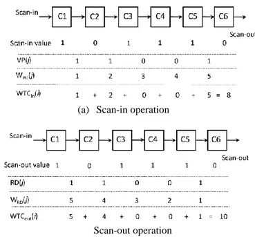
Given a test pattern and the scan-cell order for the scan chain, we can use the weighted transition count (WTC) [8] to calculate the number of scan-in and scan-out transitions generated during the scan-shift cycles. The WTC considers not only the value difference between the patterns or responses of two adjacent scan cells, but also the number of transitions that this value difference generates during the scan-shift cycles. Equation 1 and 2 define the WTCin(i) and WTCout(i) to calculate the scan-in transitions and scan-out transitions generated by the ith pattern, respectively.
(1) (1)
(2)
In equation 1 and 2, s denotes the total number of scan cells; PD(j) (RD(j)) denotes the value difference between the scan-in pattern (scan-out response) of the jth cell and the j + 1 cell; WPD(j) denotes the number of scan-in transitions generated by the pattern-value difference PD(j) when shifting in the corresponding pattern values from the scan-chain input to the j + 1 cell; WRD(j) denotes the number of scan-out transitions generated by the response-value difference RD(j) when shifting out the responses from the j cell to the scan- chain output.
In the WTC calculation, WPD(j) = j, implying that a pattern-value difference can generate more scan-in transitions if this value difference occurs closer to the scan-chain output. On the contrary, WRD(j) = s−1−j, implying that a response-value difference can generate more scan-out transitions if this value difference occurs closer to the scan-chain input. Figure 1 shows an example of the WTC computation on a 6-cell scan-chain, assuming that three value differences occur between cells (C1, C2), (C2, C3), and (C5, C6) for both the test pattern and its response.
Equation 3 calculates the total number of transitions, WTCtotal, generated by a given test set with m test patterns.
(3)
(a) Scan-in operation
Scan-out operation
Fig. 1 Calculation of scan-in and scan-out WTC.
4. SCAN-CELL REORDERING CONSIDERING ONLY RESPONSE CORRELATION
A. Detailed Steps of Reordering Scheme
We introduce a scan-cell reordering scheme, named RORC (ReOrdering considering Response Correlation), which first reduces the scan-out transitions by minimizing the response correlations while preserving all don’t-care bits in the test patterns. Then, the scan-in transitions are further minimized by specifying the don’t-care bits with MT-fill. Figure 2 shows the flow of RORC, which consists of five main steps. The detail of each step is described in the following subsections.
Fig. 2. Main steps of the proposed reordering scheme RORC.
1) Obtain Response Correlations: A simulation-based method is applied to sample the response correlations between each pair of scan cells. However, the filling of don’t-care bits in RORC is not purely random since the MT-fill technique will be applied later in RORC. Therefore, in this step, we randomly generate the scan-cell ordering multiple times, specify don’t-care bits using MT-fill based on each generated scan-cell
1
0*
s in PD jWTC
i
PD j
W
j
1
0*
s out RD jWTC
i
RD j
W
j
1 m total in out i WTC WTC i WTC i
ordering, and then collect the response correlations by
simulating the filled patterns. The number of
random-generated cell orderings used in simulation will determine the accuracy of the sampled response correlations. We use the following empirical equation to determine this number of random-generated cell orderings.
_
_
/ 50 *
_
,
Simulation Times
G Counts
P Counts
(4)
where G_Counts and P Counts denote the circuit gate count and the number of given test patterns, respectively.
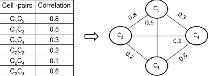
2) Construct the Correlation Graph: After obtaining the response correlations, we construct a non-directed graph, named response-correlation graph, in which a vertex represents a scan cell and the weight of each edge represents the response correlation between the adjacent vertices. Because any pair of scan cells could be placed next to each other, the response-correlation graph is a complete graph. Figure 3 shows an example of constructing a response- correlation graph with four scan cells.
Fig. 3 Construction of a response-correlation graph.
3) Find a Maximal Hamiltonian Cycle: A higher response correlation between two scan cells implies a lower probability that a response-value difference occurs between the two cells. Based on this concept, the maximum Hamiltonian cycle on the response-correlation graph implies a scan-cell ordering on which the number of value differences generated between adjacent cells is statistically minimum. Finding the maximum Hamiltonian cycle is known as the traveling salesman problem (TSP), which is NP-complete. We use a greedy TSP algorithm, which orders one vertex at a time to form the cycle. The selection criteria for the new ordered vertex are to find the vertex which has the maximum weight with the previous ordered vertex. In addition, we select the first N largest edges as the initial searching points and report the best result out of these N trials, where N denotes the total number of scan cells. The time complexity of this algorithm is Q(N3).
4) Determine Cell Ordering with Minimal WTC: In the previous step, we obtained a maximal Hamiltonian cycle on the response-correlation graph so that the number of potential response-value differences between adjacent cells can be minimized. However, to minimize the WTCout, we need to consider not only the number of response-value differences but also the positions of those value differences in the cell ordering. In Step 4, we break the given maximal Hamiltonian cycle into a Hamiltonian path, which forms the final scan-cell ordering. The breaking of the Hamiltonian cycle will affect the positions of the response-value differences and, in turn, affect the WTCout. Here, we estimate the WTCout generated by each possible breaking of the given Hamiltonian cycle and use the breaking with the minimum WTCout to form the final cell ordering.
The estimated WTCout here is obtained by replacing the RD(j) in Equation 2 with 1 minus the response correlation between cell j and j + 1. For example, the
maximal Hamiltonian cycle in Figure 3 is
C1-C2-C4-C3-C1. Figure 4 shows the estimated WTCout for all eight cases of the possible cycle breaking. The final cell ordering of the scan chain is C2-C1-C3-C4.
Fig. 4 Estimated WTCout of different scan-chain input/out.
5) Apply MT-Fill to Specify Don’t-care Bits: After the scan-cell ordering is decided in the previous step, we apply the MT-fill technique to fill the don’t-care bits of the test patterns so that the scan-in transitions based on the scan-cell ordering can be minimized. The rule of MT-fill is that a don’t-care bit is filled with the value of the first encountered specified bit when traversing from the don’t-care bit toward the scan-chain output. Refer to [8] for more details of MT-fill.
B. Experimental Results
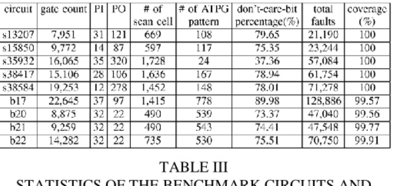
We conduct experiments on ten ISCAS and ITC benchmark circuits. Table III first shows the statistics of the benchmark circuits and their ATPG patterns generated by [24].
TABLE III
STATISTICS OF THE BENCHMARK CIRCUITS AND THEIR ATPG PATTERNS.
The following experiment compares RORC with another scan-cell reordering scheme presented in [18], which requires fully-specified test patterns before the reordering. Since RORC applies MT-fill to minimize the scan-in transitions, we apply MT-fill for [18] as well. In the following experiment of [18], we first randomly generate an initial scan-cell ordering and specify the don’t-care bits using MT-fill according to that initial ordering. Then the reordering scheme in [18] is applied to obtain the final scan-cell ordering based on the filled patterns. We repeat the above steps 100 times and report the best results for [18]. Also, we use the same TSP algorithm in both RORC and [18] to make a fair comparison.
In Table IV, Columns 3, 4, and 5 list the numbers of scan- in transitions, scan-out transitions, total scan-shift transitions, respectively. Column 6 lists the peak number of scan-shift transitions at a single scan-shift cycle. Column 7 lists the runtime in seconds. The results show that RORC can outperform [18] with an average 43.68% and 49.50% reduction to the number of scan-in transitions and scan-out transitions, respectively. The reduction to scan-in transitions first demonstrates the advantages of preserving don’t-care bits for later minimization. Also, the reduction to scan-out transitions demonstrates the effectiveness of using sampled response correlations to guide the reordering process. The reduction to peak transitions is a byproduct of the reduction to total scan-shift transitions. Note that the result reported for [18] is selected from 100 trials of random initial cell ordering. It implies that, even with MT-fill, specifying all don’t-care bits before reordering will significantly decrease the opportunity in minimizing scan-shift transitions later on and, in turn, lead to a local optimum. It also implies that the optimal cell ordering obtained by
RORC is hard to be achieved by randomly assigning the initial cell ordering of [18] for multiple times.
The runtime of [18] reported in Table IV is the runtime for 100 trials but the runtime of RORC is for only one trial. Thus, the runtime for one RORC is actually longer than the runtime for one [18]. Table V reports RORC’s runtime distribution for each benchmark circuit. Column 2 to 4 lists the runtime spent in the response-correlation sampling (Column 2), TSP algorithm (Column 3), and other computation (Column 4), respectively. Column 5 lists the total runtime. Column 6 lists the ratio of the runtime spent in correlation sampling over the total runtime. In average, 90% of the total runtime is spent on sampling the response correlations, which is actually the efficiency bottleneck of the proposed scan-cell reordering scheme.
In Table IV, the total number of scan-shift transitions is actually slightly larger than the sum of scan-in transitions and scan-out transitions. This is because we omitted the in- between transitions in Table IV, which are generated by the value difference between the first bit of a scan-in pattern and the last bit of its previous scan-out response. The percentage of in-between transitions is low compared to the scan-in and scan-out transition. It can be further reduced by a pattern- reordering scheme proposed in the next section.
TABLE IV
COMPARISONS OF GENERATED SCAN-SHIFT TRANSITIONS BETWEEN RORC AND [18].
TABLE V
RUNTIME DISTRIBUTION OF RORC (IN SECONDS).
5. PATTERN REORDERING FOR MINIMIZING IN-BETWEEN TRANSITIONS
A. Detailed Steps of Pattern Reordering Scheme
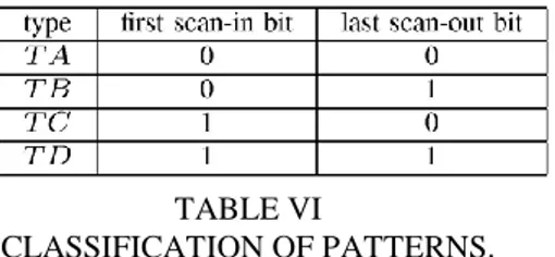
We first divide test patterns into four types, A, B, C, and D, according to the first scan-in bit of a pattern and the last scan-out bit of its response. The other bits in a pattern and its response cannot affect the number of in-between transitions. Table VI lists the classification rules for each type of patterns.
TABLE VI
CLASSIFICATION OF PATTERNS.
Next, we denote the Ai as the ith pattern in type A. The same suffix notation is applied to pattern type B, C, and D. The numbers of patterns of type A, B, C, and D are w, x, y, and z, respectively. If x > y, we reorder the patterns according to the following ordering:
1 1 2 2 1 1
w y y y x z
A A B C B C B C B B D D (5) If x < y, then we apply the following ordering:
1 z 1 1 2 2
1
y 1 zD
D C B C B
CxBxCx
C A
A
(6) The above two pattern orderings both attempt to alternately arrange one type-B pattern next to one type-C pattern as often as possible, such that the last bit of more responses can be the same as the first bit of their next pattern. Both above pattern orderings also consecutively arrange all type-A patterns or all type-D patterns next to each other. There is no in-between transition among such a consecutive sequence of type-A patterns or type-B patterns.Table VII compare the results with and without applying the proposed pattern reordering. Column 2, 3, and 4 list the number of in-between transitions, the number of total transitions, and the ratio of in-between transitions over the total transitions, respectively, without applying the proposed pattern reordering. Column 5, 6, and 7 list the corresponding results with applying the proposed pattern reordering. As the results show, the average ratio of in-between transitions can be reduced from 0.915% to 0.241% by applying the proposed pattern reordering. Also, the runtime of this pattern reordering is fast (less than 1 second for all benchmark circuits).
TABLE VII
COMPARISON ON IN-BETWEEN TRANSITIONS BETWEEN USING AND WITHOUT USING PATTERN
REORDERING.
Since the percentage of in-between transitions is much lower than that of scan-in transitions or scan-out transitions (0.241% in average), we will not individually list the number of in- between transitions in later experiments so that the focus of our scan-cell reordering schemes can be on the scan-in and scan-out transitions. We will still count in-between transitions in the total number of scan-shift transitions.
6. SCAN-CELL REORDERING CONSIDERING RESPONSE AND PATTERN CORRELATIONS
As the results shown in Table IV, RORC generates a lower number of total scan-shift transitions than [18] in all circuits but s35932. This exception may attribute to its low don’t-care-bit percentage of 37.36%. From our internal experiments, we found that a cell ordering will affect the results of the MT-fill more significantly when the don’t-care-bit percentage becomes lower. However, RORC can only reduce scan-out transitions by minimizing the response correlations between adjacent cells. It ignores the impact of the cell ordering on the number of scan-in transitions resulted from the MT-fill patterns.
In this section, we introduce another scan-cell
reordering scheme, named ROBPR (ReOrdering
considering Both Pattern and Response correlation),
which can simultaneously optimize the pattern
correlations and response correlations during the reordering process.
A. Detailed Steps of Reordering Scheme
Figure 5 shows the flow of ROBPR consisting of four main steps. The details of steps 1-3 are described in the following subsections. The detail of step 4 is the same as the step 5 in RORC and hence omitted in this section.
Fig. 5 Main steps of the proposed reordering scheme ROBPR.
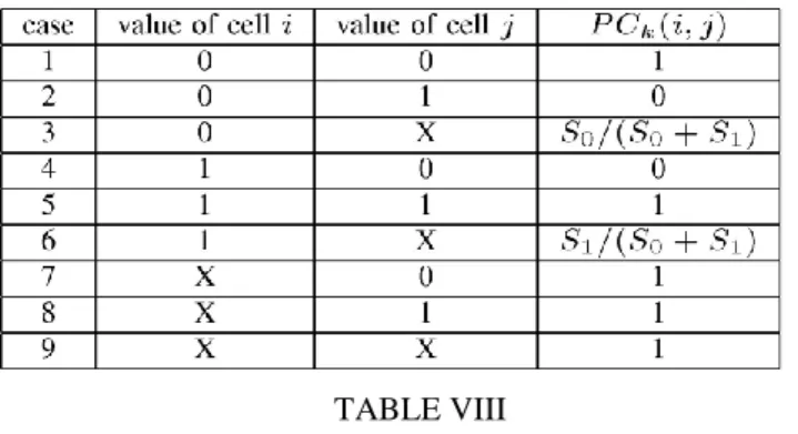
1) Obtain Pattern and Response Correlations: In order to measure the impact of a scan-cell ordering on the number of scan-in transitions, we first define the pattern correlation between cell i and cell j as the probability that the pattern values on these two cells are the same when the output of cell i is connected to the input of cell j. Note that this pattern correlation is dependent on the order of cells. For a test pattern k, Table VIII considers each combination of pattern values between cell i and cell j, and lists its corresponding pattern correlation after MT-fill (denoted as PCk (i, j)).
TABLE VIII
DIFFERENT CASES OF PATTERN CORRELATIONS BETWEEN TWO ADJACENT CELLS.
In cases 1, 2, 4, and 5, both values of cell i and j are specified bits and hence their pattern correlations can be determined immediately for test pattern k. In cases 7, 8, and 9, a don’t-care bit are placed prior to a specified bit and hence the don’t-care bit will be filled with the same value as the specified bit. In cases 3 and 6, a specified bit is placed prior to a don’t-care bit. Hence, the
value of this don’t-care bit cannot be derived immediately and has to be determined by its first encountered specified bit when traversing toward the scan-chain output. We use S0/(S0 + S1 ) (S1 /(S0 + S1 )) to represent the probability that its first encountered specified bit is a 0 (1), where S0 and S1 denote the total numbers of specified 1s and 0s in the test pattern, respectively.
After calculating the PCk (i, j) for each pattern k, the pattern correlation between cell i and cell j for the entire test set can be obtained by averaging the PCk (i, j) for each pattern k.
As to the response correlations, we use the same simulation- based method described in the Sec. IV-A1 to estimate them.
2) Construct the Directed Correlation Graph: The correlation graph constructed in ROBPR is a revised version of the correlation graph. First, this correlation graph is directed. Second, an edge in this correlation graph has two weights (Wp, Wr), where Wp and Wr represent the pattern correlation and response correlation, respectively. Figure 6 shows an example of constructing such a directed correlation graph given the pattern and response correlations between three scan cells.
Fig. 6 Construction of the directed graph based on pattern and response correlations.
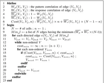
3) Find the Hamiltonian Path with Minimal WTC: Un- like RORC which finds a Hamiltonian cycle first and then breaks the Hamiltonian cycle to obtain a Hamiltonian path with minimal estimated WTCout, ROBPR uses an integrated algorithm to directly obtain the Hamiltonian path with minimal estimated W T Ctotal on the correlation graph. Figure 7 shows the proposed greedy-based algorithm, which also ordered one new vertex at a time to form such a Hamiltonian path.
When adding the nth non-ordered vertex Vnon for the Hamiltonian path, this algorithm uses a cost function Cost(Vlast, Vnon, n) to measure the impact of the new-added edge (Vlast, Vnon) on WTCtotal, which is
defined in Equation 3. In the definition of Cost(Vi, Vj , n) in Figure 7, the Wp’(Vi, Vj ) (Wr’(Vi, Vj )) actually
represents the probability that a pattern-value
(response-value) difference occurs between Vi and Vj. The n in the cost function actually represents the WPD(n) described in the WTC equation 1. The N − 1 – n in the cost function actually represents the WRD(n) described in the WTC equation 2.
Fig. 7 The proposed algorithm for finding a Hamilton path with minimal WTCtotal.
This cost function will guide the algorithm to emphasize more on the response correlation in the beginning of the ordering process and then gradually move its emphasis to the pattern correlation in the later stage of the reordering process, which exactly reflects the WTC definition in Equations 1 and 2.
B. Experimental Results
We conduct experiments for ROBPR on the same bench- mark circuits and test patterns as in Sec. IV-B. Table IX compares the results of ROBPR with the results of RORC, which considers only the response correlation during the reordering. The experimental results show that, in average, ROBPR can generate 34.87% less scan-in transitions but only 6.33% more scan-out transitions compared to RORC. This significant reduction in scan-in
transitions first demonstrates the advantage of adding the pattern correlations into consideration during the ordering process. It also shows the effectiveness of the pattern-correlation estimation listed in Table VIII.
The average reduction to the total scan-shift transitions is 12.38% by ROBPR. The 7.52% reduction to the number of peak transitions is a byproduct of the reduction to total scan- shift transitions as well. The overall result again demonstrates the benefit of considering pattern correlations and response correlations simultaneously during the reordering. In addition, the reported runtime of ROBPR is almost the same as RORC, even though ROBPR needs to collect additional information for pattern-correlations calculation. It is because the proposed algorithm in Step 3 (Figure 7) can directly find the Hamiltonian path with minimal WTCtotal, saving a step of breaking a Hamilton cycle to obtain the final ordering, such as the Step 4 in RORC.
7. SCAN-CELL REORDERING USING SCAN-DATA INVERSION
To reduce potential signal transitions, both RORC and ROBPR arrange the scan cells with a high response (or pattern) correlation next to each other. It is because a high correlation between two scan cells represents a high probability that their response (or pattern) values are the same. On the contrary, a low correlation between two scan cells means that their response (or pattern) values are most likely inverse to each other. In such a low-correlation case, if we can inverse the value of a cell before it propagates to the scan-in port of the other cell, this low correlation can be turned into a high correlation and become helpful for minimizing scan-shift transitions.
In this section, we introduce a scan-cell-reordering scheme, named SIRO (Scan-data-Inversion ReOrdering). SIRO selectively applies the inversion connection between two scan cells and hence can take advantage of both high correlations and low correlations between responses and patterns.
TABLE IX
COMPARISONS OF GENERATED SCAN-SHIFT TRANSITION BETWEEN RORC AND ROBPR
A. Detailed Steps of Reordering Scheme
Figure 8 shows the overall flow of SIRO, which consists of the following four steps.
1) Obtain Inverse Pattern and Response Correlations: In SIRO, when connecting a scan cell i to its next scan cell j, two types of connections can be made. One is direct connection, which connects the value Q of i to the scan-in port SI of j. The other type is the inverse connection, which connects the inverse value Q of i to the scan-in port SI of j. In RORC and ROBPR, we already discussed how to estimate the response and pattern correlations when using the direct connection. The focus here is to estimate the response correlations and pattern correlations when using the inverse connection.
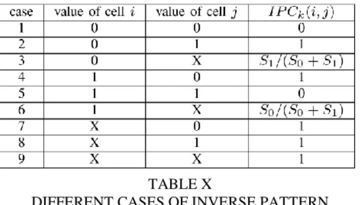
The response correlation for an inverse connection can be simply estimated by 1 minus the response correlation calculated for a direct connection. However, it is more complicated to estimate the pattern correlations for an inverse connection. This is because the MT-fill can adjust its filling of don’t-care bits according to the inverse connection or the direct connection. We first define the inverse pattern correlation between cell i and cell j for pattern k as I PCk (i, j), which is the probability that the pattern values on these two cells are the same when cell i
is inversely connected to cell j. Table X shows the inverse pattern correlation for different combinations of pattern values between cell i and cell j after MT-fill. The derivation of Table X is similar to Table VIII. The only difference is that, for an inversely connected cell pair, a transition is generated when the specified values of both cells are the same. The definition of S0 and S1 are the same as that in Table VIII.
Fig 8. Main steps of the proposed reordering schemes SIRO.
TABLE X
DIFFERENT CASES OF INVERSE PATTERN CORRELATIONS BETWEEN TWO ADJACENT CELLS.
2) Construct the Directed Correlation Graph: The correlation graph constructed in SIRO is a revised version of the correlation graph in ROBPR. The difference is that an edge in this correlation graph has two sets of weights: non-inverse set (Wp, Wr) and inverse set (I Wp, I Wr), where Wp and Wr represent the direct pattern correlation and response correlation as calculated in ROBPR, and IWp and IWr represent the inverse pattern correlation and response correlation as calculated in previous step. Figure 9 shows an example of constructing such a directed correlation graph given the inverse and non- inverse correlation sets between three scan cells.
3) Find the Hamiltonian Path with Minimal WTC: The algorithm in this step is similar to the algorithm in Figure 7, except two types of connections can be chosen in SIRO. When selecting the nth ordered cell, SIRO needs to evaluate both the cost function for a direct connection Cost(Vi, Vj, n) and the cost function for an inverse connection Costinv(Vi, Vj, n). Cost(Vi, Vj , n) is defined in ROBPR. Costinv(Vi, Vj, n) is defined as follows:
C ostinv (Vi , Vj , n) = I Wp (Vi , Vj ) × n + I Wr (Vi , Vj ) ×
(N − 1 − n) (7)
The cell with the highest cost function will be selected and the selected cell is directly or inversely connected to the next cell according to the type of the highest cost function (Cost(Vi , Vj , n) or Costinv (Vi , Vj , n)).
4) Determine the Scan-in Patterns Based on Derived Cell Ordering: Unlike the RORC and ROBPR which directly use the traditional MT-fill to determine patterns based on the derived cell ordering, the MT-fill in SIRO needs to apply a different filling rule to handle inverse connections. First, the value of a specified bit is inverse if an odd number of inverse connections are encountered before the specified bit. The specified bits remain the same if even numbers of inverse connections are encountered. Next, the don’t-care bits between the modified specified bits are filled using the traditional MT- Fill. Figure 10 shows an example of the revised MT-Fill to handle inverse connections.
Fig. 9 Construction of the directed graph based on inverse and non-inverse correlation sets.
Fig. 10 An example of the MT-fill performed in SIRO.
In Figure 10, the scan chain contains six scan cells, and three inversions occur on cell pairs (C1, C2), (C4, C5), and (C5, C6), respectively. Because C2, C3, C4, and C6 pass through odd times of inversions (1 or 3 times) during scan-in operation, the specified values are inverse before MT-fill. Then the MT-fill is applied to fill all the don’t-care bits according to the modified specified bits. Figure 11 shows the inverse connections of scan cells corresponding to the example in Figure 10. In Figure 11,
the differences with traditional architecture are that Q connects to SI while the inversions occur.
Fig. 11 Implement inverse techniques with traditional scan-chain architecture.
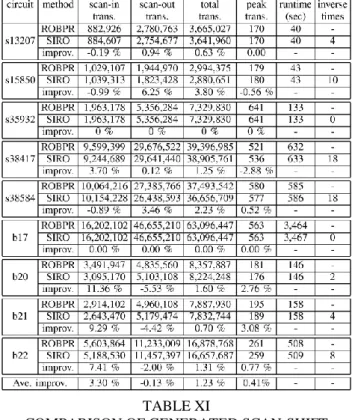
TABLE XI
COMPARISON OF GENERATED SCAN-SHIFT TRANSITIONS BETWEEN SIRO AND ROBPR.
B. Experimental Results
We conduct experiments for SIRO on the same benchmark circuits and test patterns as those used in Sec IV-B. Table XI compares the results of SIRO with that of ROBPR, which considers only the non-inverse pattern and response correlation during the reordering process. As the results show in Table XI, SIRO in average can generate 1.23% less total scan-shift transitions with almost the same runtime compared to ROBPR. However, even though RISO can generate a smaller or at least even number of scan-shift transitions for each circuit, this 1.23% average reduction is still less than our expectation before the experiment.
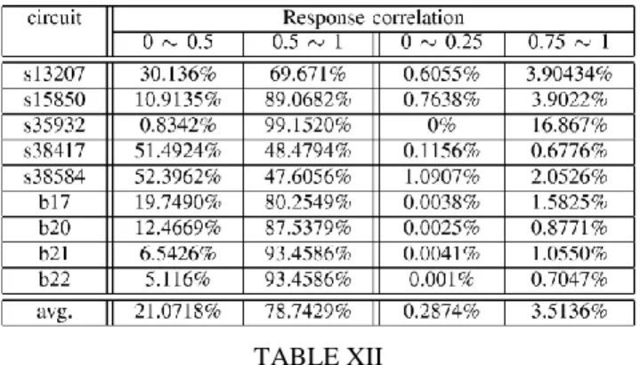
After further analysis, we found that the number of inverse connections used in each circuit is actually small (as listed in the last column of Table XI. For s35932 and b17, even no inverse connection is used by SIRO. This low usage of inverse connection means that the low correlations between scan cells in those benchmark circuits are not low enough, so that the corresponding inverse correlations cannot produce a high score for the cost function Costinv(Vi, Vj, n) used in Step 3’s greedy algorithm. This argument is further supported by the response-correlations distribution reported in Table I, where 2.05% of response correlations are larger than 0.75 but only 1.09% of response correlations are smaller than 0.25 for s38584. This trend is even more obvious for b17 as shown in Table II, where 1.58% of response correlations are larger than 0.75 but only 0.004% of response correlations are smaller than 0.25. Table XII lists the probability distributions of response correlations for each benchmark circuit.
TABLE XII
Probability distribution of high and low response correlations.
From the above experiments, we can conclude that using the inverse connections can indeed help the reduction on scan-shift transitions since the only a small number of inverse connections can achieve a 1.23% average reduction in the total scan-shift transitions. However, the amount of this reduction is determined by the ratio of low response or pattern correlations over the high ones, which is highly circuit-dependent. The reduction could be more significant if this ratio is higher.
7. SCAN CELL REORDERING CONSIDERING BOTH POWER AND ROUTING FACTORS
All above reordering schemes, such as RORC, ROBPR, and SIRO, focus on reducing the power consumption during scan- based testing. However, these reordering schemes may result in long wire length of scan paths since the connection of scan cells is determined by cells’ response or pattern correlations, not cells’ physical distance. In this section, we proposed a scan-cell reordering scheme, named PRORO (Power and Routing-Overhead ReOrdering), which combines the
ROBPR with routing consideration. The same idea can be applied to SIRO as well.
A. Detailed Steps of Reordering Consideration both Power and Routing Overhead.
In PRORO, we reorder the scan cells after the placement is done. Based on the placement result, we use the Manhattan distance between two scan cells to approximate the wire length between the two cells. When selecting the next ordered scan cell, we incorporate this approximated wire length into the cost function and hence can limit the routing overhead. In our implementation, the placement is done by a commercial back-end tool and the position of each scan cell is obtained by parsing its DEF file.
Basically, PRORO contains almost the same five steps as that of ROBPR, except some modifications to the step 2 and 3. Therefore, this subsection only shows the details of step 2 and 3. The rest steps all follow the steps in ROBPR.
1) Construct a Directed Multiple-Weight Graph Based on Response/Pattern Correlations and Routing Overhead: As mentioned, the Manhattan distance between two cells is used to represent their routing overhead. In order to make the quantity of routing overhead compatible with the quantity of the cost function regarding scan-shift power, we normalize two cells’ routing overhead (represented by the Manhattan distance) to a value between 0 to 1, which is defined as the routing weight between the two cells. We set the longest distance between any two cells as a routing weight of 1, and the shortest distance as a routing weight of 0.
Fig. 12 Construction of the directed graph based on correlations and routing effects.
The directed graph constructed in this section is a revised version of the directed graph introduced in ROBPR (Step 2 in Sec VI-A2). An edge in the graph contains three weights (Wp, Wr, Wl), where Wp, Wr and Wl represent the pattern correlation, the response correlation, and the routing weight between the two cells, respectively. Figure 12 shows an example of constructing such a directed graph given the correlation and routing weight between three scan cells.
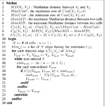
2) Find the Hamiltonian path with the minimum WTC: We use a similar greedy TSP algorithm as shown in Figure 7 except its cost function CT, which is modified as follows to control the tradeoff between scan-shift power and routing overhead:
CT (Vi , Vj , n) = (1 − β) × CP (Vi , Vj , n) + β × CR (Vi , Vj ) (8)
CR(Vi, Vj) represents the routing weight between cells Vi and Vj. CP (Vi, Vj, n) represents the cost function of scan- shift power when selecting the nth cell and ranges from 0 to 1 as well. The value of CP (Vi, Vj , n) is computed by the value of Cost(Vi, Vj , n) divided by the maximum value of Cost(Vi, Vj , n) between any two cells, where Cost(Vi, Vj , n) is defined in ROBPR (see Figure 7). The parameter β in CT (Vi, Vj, n) is call the optimization factor, which is used to control the tradeoff between scan-shift power and routing over- head. The value of β ranges from 0 to 1. If β increases, this TSP algorithm focuses more on reducing routing overhead. If β decreases, this TSP algorithm focuses more on reducing scan-shift transitions. Figure 13 shows the details of the TSP algorithm.
Fig. 13 The proposed algorithm for finding a Hamilton path optimizing power and routing overhead in PRORO.
B. Experimental Results
We conduct the following experiments to compare the results of PRORO using different optimization factors with the results of ROBPR and a scan-cell reordering scheme supported by a commercial back-end tool [25], where ROBPR only focuses on minimizing the scan-shift transitions and [25]’s scan-cell reordering only focuses on minimizing the routing overhead of scan paths after the
placement is done. In the following experiments, we first use ROBPR to obtain a scan- cell ordering and apply the APR tool in [25] to get its placement. Then both PRORO and [25]’s scan-cell reordering are performed based on this placement of ROBPR. [25]’s scan-cell reordering is performed by using the command”scan reorder” in [25]. A TSMC 0.18µm CMOS technology with 5 metal layers is used in the experiments.
Table XIII first lists the total number of scan-shift transitions generated by different scan-cell reordering schemes. For the convenience of result comparison, Table XIII normalizes the total number of scan-shift transitions of each reordering scheme by dividing it with the total number of scan-shift transitions of ROBPR, which is supposed to be the reordering scheme generating the least scan-shift transitions in this experiment.
Table XIV lists the estimated wire length of the scan paths (in µm) generated by different scan-cell reordering schemes. This estimated wire length of scan paths is measured by the summation of the Manhattan distance between any two adjacent scan cells. Similar to Table XIII, Table XIV also normalizes the wire length of scan paths of each reordering scheme by dividing it with that of [25]’s reordering scheme, which is supposed to be the reordering scheme generating the shortest wire length of scan paths in this experiment. Table XV further lists the total wire length (including the routing for both scan paths and CUT) generated by each reordering scheme after detailed route.
TABLE XIII
COMPARISONS OF SCAN-SHIFT TRANSITIONS GENERATED BY DIFFERENT SCAN-CELL REORDERING
TABLE XIV
COMPARISONS OF SCAN PATH’S WIRE LENGTH (um) AFTER GLOBAL ROUTE GENERATED BY DIFFERENT
SCAN-CELL REORDERING SCHEMES.
As the results shown in Table XIII, if only minimizing the wire length of scan paths such as tool [25]’s reordering scheme, 2.4 times the scan-shift transitions of ROBPR are generated, where ROBPR only minimizes scan-shift transitions. On the other hand, ROBPR requires 3.3 times the wire length of scan paths of tool [25]’s reordering scheme as shown in Table XIV. In fact, the wire length spent on CUT’s routing is much more than the wire length spent on scan paths’ routing. Thus, after detailed route, the total wire length of ROBPR is 1.26 times the total wire length of tool [25]’s reordering scheme as shown in Table XV.
TABLE XV
COMPARISONS OF TOTAL WIRE LENGTH (um) AFTER DETAILED ROUTE GENERATED BY DIFFERENT
SCAN-CELL REORDERING SCHEMES.
Also, the experimental results in Table XIII, XIV, and XV show that the tradeoff between scan-shift transitions
and scan path’s wire length can be controlled by PRORO with different optimization factors. Using a larger optimization factor, PRORO can reduce more wire length of scan paths but generate more scan-shift transitions. When the optimization factor equals 0.5, PRORO generates 12% more scan-shift transitions compared to ROBPR but only requires 7% total wire length after detailed route, which is an acceptable level of routing overhead as long as the design is not intensively routing-congested.
Another reason to sacrifice the wire length of scan paths for the scan-shift power is that the for advanced process technologies, the violation of hold-time constraints on scan paths occurs more often than the violation of setup-time constraints. Designers even intentionally increase the wire length of some scan paths to meet the hold-time constraint instead of applying a scan-cell reordering to reduce its wire length. Therefore, the motivation of reducing wire length on scan paths may not be as strong as that in the old process technologies.
三、結論
In this project, we first presented a scan-cell reordering technique which can simultaneously reduce scan-shift transitions based on the response correlations and preserve don’t-care bits in the test patterns for a later minimization of scan-in transitions using MT-fill. Second, we considered both the response correlation and pattern correlations during the cell reordering process to further reduce the scan-in transitions generated by MT-fill (Section VI). Next, we utilized the inverse connection between scan cells to turn a low correlation into a high one and developed a corresponding scan- cell reordering scheme to consider those inverse correlations. Last, we incorporated the routing overhead of scan paths into the cost function of our scan-cell reordering and hence the trade-off between scan path’s routing overhead and the number of scan-shift transitions can be controlled by a user-specified factor. In addition, a post-process pattern- reordering scheme was also proposed to minimize the in- between transitions. A series of experiments were conducted to compare the proposed schemes with a previous reordering scheme [18] and a commercial tool’s reordering scheme [25]. The experimental results demonstrated the effectiveness and efficiency of each of the proposed scan-cell reordering schemes
四、參考文獻
1. M. Bushnell and V. Agrawal. Essentials of Electronic Testing. Kluwer Academic Publishers, 2000.
vlsi devices. Proc. 11th IEEE VTS, pages 4–9, January 1993.
3. P. Girard. Survey of low-power testing of vlsi circuits. IEEE Design and Test of Computers, 19(No 3):82–92, May-June 2002.
4. S. Remersaro and X. L. et al. Preferred fill a scalable method to reduce capture power for scan based designs. Proc. Int. Test Conf., 2006.
5. X. Wen and Y. Y. et al. On low-capture-power test generaion for scan testing. Proc. VTS, pages 265–270, 2005.
6. R. Sankaralingam and N. A. Touba. Controlling peak power during scan testing. Proc. VTS, pages 153–159, 2002.
7. A. Chandra and R. Kapur. Bounded adjacent fill for low capture power scan testing. Proc. VTS, pages, 2008. 8. R. Sankaralingam and R. R. O. et al. Static compaction
techniques to control scan vector power dissipation. Proc. VTS, pages 35–40, 2000.
9. G. Mrugalski and J. R. et al. New test data decompressor for low power applications. Proc. DAC, pages 539–544, 2007.
10. S. Lin and C. L. et al. A multilayer data copy scheme for low cost test with controlled scan-in power for multiple scan chain designs. Int. Test Conf., 2006.
11. O. Sinanoglu and A. Orailoglu. Modeling scan chain modifications for scan-in test power minimization. Int. Test Conf., 2003.
12. Y. B. et al. A gated clock scheme for low power scan testing of logic ics or embedded cores. Proc. 10th Asian Test Symp. (ATS01), pages 253–258, 2001.
13. P. Rosinger and B. A.-H. et al. Scan architecture with mutually exclusive scan segment activation for shiftand capture-power reduction. IEEE Transactions on Computer-Aided Design (TCAD), 23(7):1142–1153, July 2004.
14. L. Whetsel. Adapting scan architectures for low power operation. Proc. IEEE Int. Test Conf., pages 863–872, 2000.
15. J. Saxena and K. M. B. et al. An analysis of power reduction techniques in scan testing. in Proc. IEEE Int. Test Conf., pages 670–677, 2001.
16. T. Huang and K.-J. Lee. A token scan architecture for low power testing. Proc. Int. Test Conf., pages 660–669, 2001. 17. R. Sankaralingam and B. P. et al. Reducing power dissipation during test using scan chain disable. Proc. 19th VLSI Test Symp. (VTS 01), pages 319–324, 2001. 18. Y.Bonhomme and P. et al. Power driven chaining of
flip-flops in scan architectures. Int. Test Conf., pages 796–803, 2002.
19. V. Dabholkar and S. C. et al. Techniques for reducing power dissipation during test application in full scan circuits. IEEE Transactions on CAD, December 1998. 20. Y. Bonhomme and P. G. et al. Efficient scan chain design
for power minimization during scan testing under routing
constraint. IEEE Int. Test Conf., pages 488–493, 2003. 21. Y. Bonhomme and P. G. et al. Design of
routing-constrained low power scan chains. Proc. DATE, pages 62–67, 2004.
22. S. Makar. A layout-based approach for ordering scan chain flip-flops. Proc. of the IEEE Int. Test Conf., pages 341–347, 1998.
23. M. Hirech and J. B. et al. A new approach to scan chain reordering using physical design information. IEEE Int. Test Conf., pages 348–355, 1998.
24. Synopsys tetramax atpg user guide version x-2005.09. 25. Cadence encounter product version 5.2.3 June 2006.