應用於時滯系統之輸出回授積分型順滑模態控制

國

立

交

通

大

學

電控工程研究所

博 士 論 文

應用於時滯系統之輸出回授積分型順滑模態控制

Output Feedback Integral Sliding Mode Control Applied to

Time-Delay Systems

研 究 生：丁桓展

指導教授：陳永平 博士

張浚林 博士

應用於時滯系統之輸出回授積分型順滑模態控制

Output Feedback Integral Sliding Mode Control Applied to

Time-Delay Systems

研 究 生：丁桓展 Student：Huan-Chan Ting

指導教授：陳永平 教授 Advisors：Prof. Yon-Ping Chen

張浚林 教授

Prof. Jeang-Lin Chang

國 立 交 通 大 學

電 控 工 程 研 究 所

博 士 論 文

A Dissertation

Submitted to Institute of Electrical Control Engineering College of Electrical and Computer Engineering

National Chiao Tung University in partial Fulfillment of the Requirements

for the Degree of Doctor of Philosophy

in

Electrical Control Engineering May 2011

Hsinchu, Taiwan, Republic of China

應 用 於 時 滯 系 統 之 輸 出 回 授 積 分 型 順 滑 模 態 控 制

學生：丁桓展

指導教授

：

陳永平教授

張浚林教授

國立交通大學電控工程研究所博士班

摘

要

基於線性多輸入多輸出系統，在部分參數不確定且受到外界未知干擾之環境，本論 文提出一動態輸出回授積分型順滑模態控制法則，使受控系統穩定並抑制非匹配干擾之 影響。順滑模態控制為一強健非線性的控制方法，先設計一穩定之順滑平面，再設計控 制輸入使系統在有限時間內進入該平面，具有設計簡單、可消除匹配性雜訊等優點。當 系統只有部分狀態或是輸出訊號可量測，應用於此類系統之傳統輸出回授順滑模態控制 器存在著受限於系統結構的控制器合成問題，且只能滿足區域性的逼近與順滑條件。本 論文採用積分型順滑平面，可保留順滑模態控制原有之優點，並解決控制器合成問題， 當系統進入順滑平面後也可提供一自由度去抑制非匹配型干擾之影響。另外為了滿足全 域逼近與順滑條件，在控制輸入中設計了一個適應性法則，計算部份未知量的範數上 限。此動態輸出回授積分型順滑模態控制法則，經過修正後亦可應用於參數不確定且受 到外界未知干擾之時滯系統。針對於固定但未知延遲時間之狀態延遲時滯系統，沿用輸 出回授積分型順滑平面之結構，並加入一全階補償器以完成動態控制器之設計。當系統 進入順滑平面，利用一強健干擾抑制分析技術可以推理出一線性矩陣不等式作為穩定性 與保證干擾抑制效能的充分條件；若修正補償器結構，則該線性矩陣不等式可分解為兩 個維度較小之代數 Riccati 不等式以利計算，兩種不等式之解皆可用來決定順滑平面、 補償器、控制器之參數。當延遲時間未知且時變，讓系統在某些延遲時間造成不穩定， 使得控制難度大幅提升。利用上述動態輸出回授積分型順滑模態控制器架構，本論文亦 針對此複雜系統完成穩定性充分條件分析與控制器設計。

Output Feedback Integral Sliding Mode Control Applied to Time-Delay

Systems

student：Huan-Chan Ting

Advisors：Dr. Yon-Ping Chen

Dr. Jeang-Lin Chang

Institute of Electrical Control Engineering

National Chiao Tung University

ABSTRACT

For linear multi-input multi-output uncertain systems with external unknown disturbances, this thesis proposed a dynamic output feedback integral sliding mode control method to stabilize the system and suppress the effect of mismatched disturbances. The advantages of sliding mode control are its simple design procedure, great robustness against matched disturbances, etc. As part of system states or outputs are only measurable, conventional output feedback sliding mode controllers involved a synthesis problem by a structural constraint and ensured the approaching and sliding condition locally. The thesis adopted an integral sliding surface to improve the controller synthesis problem, reserved inherent benefits of sliding mode control, and offered an extra degree of freedom to suppress the effect of mismatched disturbances when the system is in the sliding mode, simultaneously. For satisfying the approaching and sliding condition globally, an adaption law was added in the controller to estimate the bound of part of unknown terms. The proposed control method can be modified to apply to uncertain time-delay systems with disturbances. For state delays with a fixed and unknown delay time, combined the output feedback integral sliding mode technique with a full-order compensator can complete the dynamic controller design. Since the system is in the sliding mode, using the property of robust disturbance attenuation can derive a linear matrix inequality as a sufficient condition for the stability; this linear matrix inequality can be decomposed into two smaller algebraic Riccati inequalities by modifying the structure of compensator. Solutions to two types of inequalities can both determine parameters of sliding surface, compensator, and controller. In the case of time-varying and unknown delay time, some delay times caused the instability of system and worsened the difficulty designing the controller. The proposed structure of dynamic sliding mode control can also complete the stability analysis and control law design for systems with time-varying delay.

誌 謝

首先感謝指導教授 陳永平老師、 張浚林老師於學生多年來碩博士修業期間的細心 指導，在治學方法、求學態度和待人處世多所啟迪，惠我良多，謹向兩位老師獻上最誠 摯的謝意。同時感謝口試委員 徐國鎧老師、 蘇武昌老師、 鄭志強老師、 楊谷洋老師、 徐保羅老師及 梁耀文老師寶貴的意見與指正，使本論文更臻完整。 親愛的家人是我最大的支柱，父母給予我全力的栽堷，讓我能無後顧之憂地專心於 課業，若我能有所成就，皆歸功於您們；成長與學習的過程中還有妻子及可愛的兒子彥 智的支持與陪伴，讓我擁有富足的心靈寄託；兩位弟弟以及五專同學 SB 們也在生活中 陪伴我、給予我鼓勵，謝謝你們。 最後也要感謝實驗室的伙伴們，世宏學長與現役學弟們，文俊、文榜、澤翰、榮哲、 孫齊、崇賢、振方、咨偉，以及過去相知相惜的已畢業眾學長姊、學弟妹，感謝大家於 學業和生活上的互相照顧，共同度過甘苦的研究所歲月，更豐富了我的求學時光。 丁桓展 100 年 5 月

Table of Contents

Chinese Abstract

i

English Abstract

ii

Acknowledgement

iii

Table of Contents

iv

List of Figures

vi

Symbols

viii

I. Introduction

1

1.1

Sliding Mode Control

1

1.2 Time-Delay

Systems

3

1.3 Motivation

5

1.4 Contribution

6

1.5

Organization of Thesis

8

II.

Output Feedback Sliding Mode Control

9

2.1 Problem

Formulation

9

2.2

Output Feedback Sliding Mode Controller Design

10

2.2.1

System Decomposition and Analysis

10

2.2.2

Sliding Mode Controller Synthesis

14

2.3 Summary

20

III.

Output Feedback Integral Sliding Mode Control

22

3.1 Problem

Formulation

22

3.2

Dynamic Output Feedback Sliding Mode Control

24

3.2.1

Integral Sliding Surface Design

24

3.2.2

Integral Sliding Surface Design for

d

 

t L2

30

3.2.3

Control Law Synthesis

33

3.3 Numerical

Examples

37

3.4 Summary

48

IV.

Output Feedback Integral Sliding Mode Control for

Time-Delay Systems

49

4.1 Problem

Formulation

49

4.2

Integral Sliding Surface and Sliding Mode Controller

51

4.3

Robust Stability in the Sliding Mode for

Delay-Independent Condition

53

4.3.1

Robust Disturbance Attenuation by LMI

54

4.3.2

Robust Disturbance Attenuation by Algebraic Riccati

Inequalities

61

4.4

Robust Stability in the Sliding Mode for

Delay-Dependent Condition

83

V Conclusion

96

5.1 Concluding

Remarks

96

5.2 Future

Works

97

Bibliographies

98

Appendix 1

105

Appendix 2

108

Vita

114

List of Figures

Chart 2.1 System state responses in Example 2.1 ···19

Chart 2.2 System output responses in Example 2.1···19

Chart 2.3 Sliding vector in Example 2.1 ···20

Chart 2.4 System input response in Example 2.1 ···20

Chart 3.1 System states in Example 3.1 ···39

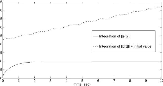
Chart 3.2 Norm of states and its upper bound in Example 3.1 ···40

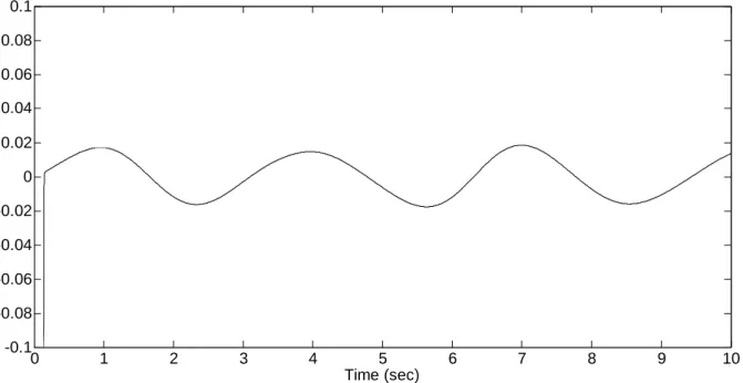
Chart 3.3 Norm of Mz

 

t and its upper bound 

 

t in Example 3.1 ···40

Chart 3.4 System outputs in Example 3.1 ···41

Chart 3.5 System inputs in Example 3.1 ···41

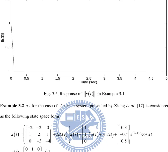
Chart 3.6 Response of s

 

t in Example 3.1 ···42

Chart 3.7 System states x t₁

 

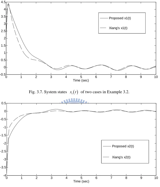
of two cases in Example 3.2 ···44

Chart 3.8 System states x t₂

 

of two cases in Example 3.2 ···44

Chart 3.9 System states x t₃

 

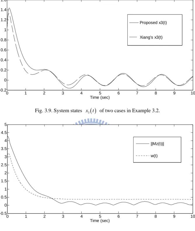
of two cases in Example 3.2···45

Chart 3.10 Norm of Mz

 

t and its upper bound 

 

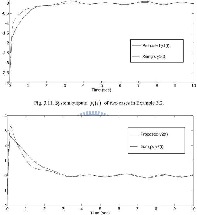
t of our proposed method in Example 3.2 ···45

Chart 3.11 System outputs y t₁

 

of two cases in Example 3.2···46

Chart 3.12 System outputs y t₂

 

of two cases in Example 3.2 ···46

Chart 3.13 Performance of robust disturbance attenuation of our proposed method in Example 3.2 ···47

Chart 3.14 System inputs u t

 

of two cases in Example 3.2 ···47

Chart 3.15 Response of s t

 

in our proposed method in Example 3.2 ···48

Chart 4.1 Flowchart for solving parameters K and L by an LMI of controller and compensator ···58

Chart 4.2 System states in Example 4.1 ···62

Chart 4.3 System outputs in Example 4.1 ···62

Chart 4.4 Performance of robust disturbance attenuation in Example 4.1···63

Chart 4.5 Sliding functions in Example 4.1 ···63

Chart 4.6 Response of s

 

t in Example 4.1 ···64

Chart 4.7 Trajectories of e

 

t in Example 4.1···64

Chart 4.8 System inputs in Example 4.1 ···65

Chart 4.9 Flowchart for solving parameters K and L by algebraic Riccati inequalities of controller and compensator ···70

Chart 4.10 System states x t₁

 

of two cases in Example 4.2···73

Chart 4.12 System states x t₃

 

of two cases in Example 4.2 ···74

Chart 4.13 System output y t₁

 

of two cases in Example 4.2 ···75

Chart 4.14 System output y t₂

 

of two cases in Example 4.2···75

Chart 4.15 Performance of robust disturbance attenuation of our proposed method in Example 4.2 ···76

Chart 4.16 Responses of s

 

t of two cases in Example 4.2 ···76

Chart 4.17 Control inputs u t₁

 

of two cases in Example 4.2 ···77

Chart 4.18 Control inputs u t₂

 

of two cases in Example 4.2···77

Chart 4.19 System states in Example 4.3 ···80

Chart 4.20 System outputs in Example 4.3 ···80

Chart 4.21 Performance of robust disturbance attenuation in Example 4.3···81

Chart 4.22 Sliding functions in Example 4.3 ···81

Chart 4.23 Response of s

 

t in Example 4.3 ···82

Chart 4.24 Trajectories of e

 

t in Example 4.3···82

Chart 4.25 System inputs in Example 4.3 ···83

Chart 4.26 System states in Example 4.4 ···90

Chart 4.27 System outputs in Example 4.4 ···90

Chart 4.28 Performance of robust disturbance attenuation in Example 4.4···91

Chart 4.29 Sliding function s t₁

 

in Example 4.4···91

Chart 4.30 Sliding function s t2

 

in Example 4.4 ···92

Chart 4.31 Response of s

 

t in Example 4.4 ···92

Chart 4.32 Responses of e

 

t in Example 4.4···93

Chart 4.33 Control input u t₁

 

in Example 4.4···93

Symbols



:

Collection of real numbers 

:

Collection of complex numbers

2

L

_:

Hilbert space of matrix-valued (or scalar-valued) function

n

I

_:

_{Identity matrix of size n n}

0 : Zero matrix with appropriate dimension

T

A

:

Transpose of the matrix A

1 

A

:

Inverse of the matrix A



A

:

Pseudo inverse of the matrix A

 

 A

_:

_{Eigenvalues of the square matrix A}

 

min

 A

_:

_{Minimum eigenvalue of the square matrix A}

 

max

 A

_:

_{Maximum eigenvalue of the square matrix A}

x

_:

_{Absolute value of the scalar x}

 

t

x

_:

_{2-norm of the vector x at time t}

A

:

2-norm of the matrix A defined as max

2 2 Ax x 

:

Equal to by definition

 

t

x

:

Time derivative of the vector x

 

t , i.e. x

 

t dx

 

t dt

 

diag 

_:

_{Diagonal matrix with the element} 

 

 A

_:

_{Range space of A}



_:

_{Union between two sets} 

_:

Intersection between two sets



:

Empty set

LMI

:

Linear Matrix Inequality LTI

:

Linear Time-Invariant MIMO

:

Multi-Input, Multi-Output

I. INTRODUCTION

In practice, most of system state signals cannot be measured fully to complete a state feedback control scheme. For the same system suffering uncertainties and external disturbances, output feedback sliding mode control method can reserve the original advantages to regulate the system behavior and avoid the design complexity of other robust output feedback control approaches. In contrast with other complex stability criteria, the approaching and sliding condition is simpler as a sufficient condition ensuring the stability while the system enters the stable sliding surface in a finite time.

Time-delay phenomenon means that parts of system states, inputs, or outputs affect the system after a fixed time, or random but finite period. There exists this phenomenon in several various practical systems, such as chemical processes, electrical networks, nuclear reactors, biological reactions, economic models, etc. Therefore controller designs for continuous-time time-delay systems are important and necessary.

1.1 Sliding Mode Control

Sliding mode control [1-28] is one of efficient robust control approaches to stabilize systems in the presence of external disturbances and interior uncertainties. It is well known for the complete invariance to matched disturbances and uncertainties. The design procedure normally follows the rule: 1) choose a stable manifold so-called sliding surface; 2) design a nonlinear switching controller satisfying the approaching and sliding condition such that the system enters the sliding surface in a finite time. The simple and explicit design procedure is another advantage of sliding mode control. Based on Utkin’s research [1], the relative papers are continuing presented over a couple of decade. Edwards and Spurgeon [2] contributed the analysis and complete introduction of sliding mode methods, state and output feedback controllers, observers, and other applications. Since the system states are all available, researchers have proposed many significant reports [3-6]. For instance, Chiang and Chiu [5]

presented a sliding mode control method based on a TS recurrent fuzzy neural network to stabilize the time-delay systems and compensate system uncertainties effectively. In the field of output feedback sliding mode control methods [7-14], previous researches have designed the output feedback controllers via sliding mode technique to stabilize multivariable plants with matched uncertainties. Early on, Zak and Hui [7] developed an algorithm for output-dependent sliding surface design of uncertain systems, using the eigenstructure method. Yallapragada et al. [8] addressed the reaching problem for the static output feedback sliding mode controller design. Thereafter, Kwan [9] presented an adapted dynamic output feedback controller to remove two major limits from the scheme in [7]. Yan et al. [14] applied an effective sliding mode design technique using output only to control the systems with disturbances.

However, the abovementioned papers considered the matched uncertainty and disturbance only. Unlike the matched case, any mismatched uncertainty and external disturbance always affect the system performance even if the plant is in the sliding mode. As a result, the existence condition and robust stability for using an output feedback sliding mode controller to tackle a system with the mismatched uncertainty and disturbance are worth further investigation. Choi [15] proposed a static output-dependent sliding surface design developed from LMI technique [29], in which a class of system considered both matched and mismatched uncertainties. Further, Park et al. [16] extended Choi’s method and proposed a dynamical output feedback variable structure control law to deal with the same problem. Since the dynamics of the sliding surface is always related to the unmeasured system states, the high gain control in [15] was introduced to maintain the global convergence. Upon examining the static output feedback control, Xiang et al. [17] applied an iterative LMI technique to avoid the high gain problem. To prepare for obtaining a bounded L gain ₂

controller which can guarantee the system stability with robust performance. Lewis [19] used the eigenvalue perturbation analysis for an uncertain matrix to guarantee the closed-loop stability. Pai and Sinha [20] used the small gain theorem to analyze the behavior of closed-loop system with parameter uncertainties. Although the advantages of applying LMI technique to output feedback sliding mode control for uncertain systems have been addressed explicitly in these aforementioned papers, the solutions including the constrained LMIs [15-16] or a set of LMIs [18, 21] are difficult to obtain.

Recent researches [22-26] have studied a control scheme called integral sliding mode control, in which an integral controller is added to a sliding mode controller. The main advantages of integral sliding mode controller are to offer the robustness of system stability and the elimination of steady state error within step inputs. Based on the integral sliding mode control structure, several researchers [23-25] developed different observer design methods to accomplish the estimation. In observer-based approaches, the proper observer gain selection which gives reasonable estimation both in steady state and transient state is a difficult task. Since the controlled systems usually involve parameter uncertainties and external unknown disturbances, the use of state observers may reduce robustness. Consequently, it is important to study the integral sliding mode control using output information only for uncertain systems.

1.2 Time-Delay Systems

For the stability analysis of time-delay systems, two kinds of conditions can be adopted — delay-independent and delay-dependent conditions. When delayed states with an unknown but bounded constant delay time are independent of the original stability of systems, the systems satisfy the so-called delay-independent condition within a simple rule assuring the stability of closed-loop systems. If the system belongs to the delay-dependent condition, delayed states with part or all of delay times will cause the instability of system whether the delay time is fixed or time-varying. This condition also brings the complexity and difficulty

deriving a sufficient condition of the stability of closed-loop systems. Since time-delay terms frequently induce the system instability and bad performance, the analysis and control of time-delay systems have been an interesting topic over the past decades whether state, input, or output delays.

Focusing on the state delay systems, researchers [3-5, 12-14, 27-28, 30-52] had presented many effective state feedback control methods to various system models. Xia and Jia [3] carried out a robust control method comprising of the sliding mode control and LMI technique for uncertain time-delay systems with matched disturbances. Lee et al. [32] developed a control method based on the receding horizon concept to stabilize the closed-loop system and to assure the H norm bound from the disturbances to the controlled outputs. For a continuous linear state-delay system involving a class of integral term, Santos and Mondié [33] proposed an iterative procedure to complete their state feedback controller design. Wang

et al. [34] designed a state feedback control law of time-delay systems with system

uncertainties and matched unknown nonlinear terms. They combined the LMI technique and adaptive parameter searching law to the controller design ensuring the stability of the closed-loop system. Chen and Chen [35] presented an LMI-based state feedback controller and a disturbance observer to stabilize linear state-delay systems with uncertainties and matched disturbances.

Providing the obtainable system states partly, state observers [36-40] and output feedback controllers [12-14, 28, 41-43, 48-52] are both feasible schemes to regulate time-delay systems. In the field of state observers, Darouach [39-40] have recently developed an observer methodology to estimate states of linear time-delay systems with noises and mismatch disturbances. On the other hand, in the field of output feedback control methods, Niu et al. [12] extended an observer-based sliding mode control using LMI technique to regulate uncertain time-delay systems. Pai [28] proposed a Luenberger observer-based output

feedback controller for a class of nonlinear uncertain state-delayed systems with matched uncertainties and disturbances. The controller was comprised of integral sliding mode technique and solutions to an LMI, which switching gain parameters were calculated by adaptation laws. Fridman and Shaked [41] described explicitly a significant H control

method using the descriptor system transformation for time-delay systems with mismatched external disturbances and measurement noises. The descriptor system transformation can simplify the analysis of time-delay systems and effectively perform the disturbance attenuation. As a result, the stability analysis [44-47] and various controller designs [48-52] of time-delay systems are still interesting topics so far.

1.3 Motivation

There exists two difficulties in the design of output feedback sliding mode control. The first difficulty is a synthesis problem. Synthesizing a control law using the outputs only is significant since the derivative of the sliding surface is always involved with the unmeasured system states. For resolving the synthesis problem, a normal strategy is to add an extra constraint on the controller parameters. The existence of controller parameters is constrained by the extra constraint simultaneously. The local stability is another problem. In the conventional output feedback sliding mode control, the dynamics of sliding surface always involves unknown state function as an obstacle to complete the controller using output information only. Common strategies dealing with this problem adopted the assumption in which the system trajectories are close to the origin or high-gain control forces covering the effect of unknown states. Unfortunately, these strategies have no ability to complete the global stability and increase the conservation.

Focusing on the case of state-delay, the state delayed for a fixed or varying time usually worsened the performance even caused the instability. In frequency domain the delay term can be transformed into an exponential function with delay time. As a result, the

corresponding controller can be designed easily in the frequency domain but very difficult to implement in the time domain. On the other hand, since a time-delay system is subject to uncertainties and disturbances, the robust controller design will become more complex and the related stability condition will be more difficult to fulfill. A sliding mode control method which has improved the previous two problems, within such features as uncomplicated design procedure and strong robustness against the matched unknown terms, is a proper and feasible candidate to complete the controller design of time-delay systems with less design difficulty in the time domain.

1.4 Contribution

For modifying two problems mentioned above in output feedback sliding mode control, this thesis develops a dynamic output feedback integral sliding mode control method with the robust stability guaranteed for linear MIMO systems within mismatched norm-bounded uncertainties along with disturbances and matched nonlinear perturbation. The main advantages of using the integral sliding surface are that, once the system is in the sliding mode, the effect of matched perturbation can be completely eliminated and the robust stability problem of the closed-loop system becomes a standard output feedback controller design problem for a system with mismatched uncertainty and disturbance. Applying H control for

the stability analysis, the proposed method can guarantee robust stability where the existence condition is determined by solving an algebraic Riccati equation involving with the original system parameters. When the number of outputs is equal to the number of inputs and the mismatched disturbance is slowly time-varying, the system outputs are proved to finally approach zero because of the integral action. Without requiring any coordinate transformation, the proposed method is a straightforward design scheme and the controller parameters can be easily solved by the algorithm proposed by Gadewadikar et al. [53-54] or the LMI technique [29]. If the mismatched disturbance is defined in L -norm space, the proposed control ₂

algorithm can satisfy the robust disturbance attenuation and guarantee robust stability as the consistent algebraic Riccati equation has a solution. Introducing an additional dynamics into the control law using output information only, the proposed controller can satisfy the global reaching and sliding condition and obtain the closed-loop stability. Although the dynamic output feedback controller raises control complexity, the magnitude of control input in the proposed method is more effectively reduced in comparison with that in the other papers [15-17].

Based on the proposed integral sliding mode control technique, the related controller design for uncertain time-delay systems with mismatched disturbances is presented. An auxiliary integration function is used to increase a degree of freedom of the system in the sliding mode and to suppress the effect of mismatched disturbances. Moreover, the controller design combined with a full-order compensator for time-delay systems also improves the synthesis problem in traditional output feedback sliding mode control methods. Since mismatched disturbances cannot be eliminated completely even the system is in the sliding mode, the disturbance attenuation technique [55-57] can reduce the effect from mismatched disturbances to the controlled outputs acting on a system to an acceptable level over all frequencies. Consequently, an LMI is derived as a sufficient condition of robust stability and its solutions are used to determine parameters of compensator and controller simultaneously. Modifying the structure of compensator can obtain a set of algebraic Riccaiti inequalities as another stability condition. Solutions to the Ricccati inequalities can also obtain the controller parameters.

The controller design for time-delay systems with a time-varying state delay has been derived within the delay-dependent condition. In the delay-dependent condition, the system is stable for part of unknown delay time and vice versa, i.e. the system stability depends on delay times. For such time-delay systems with mismatched disturbances and uncertainties, an

output feedback integral sliding mode control law combined with a compensator is completed in this thesis. An LMI as a sufficient condition of robust disturbance attenuation is derived successfully.

1.5 Organization of Thesis

The sliding mode controller using output information only [2] is introduced in Chapter II. Edwards and Spurgeon [2] contributed a complete analysis for an output feedback sliding mode control and related applications in their book. Chapter III proposed the dynamic output feedback integral sliding mode controller of uncertain systems with matched and mismatched disturbances. Based on the research of integral sliding mode control technique, the output feedback controller with a compensator is applied to time-delay systems with mismatched uncertainties and disturbances in Chapter IV. This chapter discusses two kinds of sufficient conditions guaranteed the property of robust disturbance attenuation. For the case of time-varying delay within delay-dependent condition, the same chapter derived the dynamic output feedback integral sliding mode control algorithm for such disturbed time-delay systems correspondingly. The final chapter comments the overall concluding remarks and some future works.

II. OUTPUT FEEDBACK SLIDING MODE CONTROL

In practice, state variables of most systems are not fully observable. As part of state variables is only measurable, the corresponding controller design is more difficult than the conventional state feedback controller design. Since output variables are only available, referring to [2], this chapter describes the output feedback sliding mode controller and analyzes its merits/demerits. After introducing the target system and some assumptions, section 2.2 presents the sliding mode controller using output variables directly and the corresponding sliding vector.

2.1 Problem Formulation

Consider a continuous-time LTI system as

 

 



 







 

 

, , t t t t t t     x Ax B u f x u y Cx  (2.1)

where x is the unmeasurable system state vector, n u is the control input vector, m

p



y  is the measurable output vector, and f x u



, ,t



m is consisted of the matched uncertainties and disturbances. The real constant matrices A, B, and C are known and with

appropriate dimensions. Since the outputs are the only available signals, next section will present an output-dependent sliding vector design method and then the control algorithm involving the information of outputs is designed to satisfy the stability condition and to force the controlled system (2.1) to enter the sliding mode. Before introducing main results, the following four assumptions are fulfilled throughout this chapter.

Assumption 2.1: The matched term f x u



, , t



is norm-bounded as



, ,t



k1

 

t 

 

,t

f x u u y (2.2)

where 

 

y,t is a known function :_p  and _ 0  . k₁ 1

open left-half complex plane, i.e., the triple



A B C, ,



is minimum phase.

Assumption 2.3: The pairs



A B,



and



C A,



are controllable and observable,

respectively. Matrices B and C are full rank, rank

 

B m and rank

 

C  p.

Assumption 2.4: The number of output variables is not smaller than input variables, p . m

Moreover, the relative degree of system (2.1) is one, i.e. rank

 

CB m.

2.2 Output Feedback Sliding Mode Controller Design

2.2.1 System decomposition and analysis

Define a transformation matrix as

T c c        N T C (2.3)

where N_cn n p whose columns span the null space of C. Changing the coordinates

c

xT x, the output matrix is transformed into C  0 I_p_. The input matrix in the transformed system is given by 1

2 c c        B B B where   1 n p m c    B  . Since matrix B_c2p m

is full row rank due to CBB and Assumption 2.4, the left pseudo inverse of c2 B is c2 defined as B_c†₂ 



B B_cT_{2 c2}



1B and there exists an orthogonal matrix _cT₂ Tp p such that

2 2 T c        0 T B B (2.4) where ₂ m m

B  is invertible and T is full rank. Further the second transformation matrix is defined as † 1 2 n p c c b _T          I B B T 0 T . (2.5)

system matrices, 11 12 21 22        A A A A A , ₂        0 B B , and C 



0 T



(2.6)

where A₁₁n m   n m and remaining matrices in A are partitioned to appropriate dimensions. Defining a matrix Fm p with full rank and multiplying it to C can obtain



 

1 1 2



  FC 0 FT F C F (2.7) where



F₁ F₂



FT, F₁m p m, ₂ m m F  , and 1  p m  C  0 I . (2.8)

As a result, FCBF B and _{2 2} F is invertible because of ₂ rank

 

CB rank

 

F m . Notice that the pair



A B C, ,



in (2.6) can be viewed as a system used in sliding mode controller design [2], and the reduced-order sliding mode motion is dominated by the stable system matrix A , ₁₁s 1 11 11 12 2 1 1 11 12 1 s _    A A A F F C A A KC  (2.9)

where K F F . From (2.9) it is a static output feedback problem to design K stabilizing ₂1 ₁

11 12 1

A A KC . For checking the controllability of the pair



A₁₁,A₁₂



, the following relationship within (2.6) is established,

















11 12 21 22 2 11 12 rank rank rank s s s s m n       _{ }           I A A 0 I A B A I A B I A A (2.10)

for all s . It can conclude that rank





sIA₁₁ A₁₂





 n m and



A₁₁,A₁₂



is controllable. On the other hand, for ensuring the observability of



C A₁, ₁₁



, the detail of A ₁₁

1111 1112 11 1121 1122        A A A A A (2.11)

where A₁₁₁₁n p   n p and the other matrices in A are partitioned accordingly. Hence ₁₁

the rank test can be written as

1111 1112 11 1121 1122 1 1111 1121 rank rank rank p m s s s s p m        _  _{ }  _ _     _ _       _{ }      I A A I A A I A C 0 I I A A (2.12)

for all s. Consequently, the observable pair



A₁₁₂₁,A₁₁₁₁



is a sufficient condition of the observability of the pair



C A₁, ₁₁



. If the pair



A₁₁₂₁,A₁₁₁₁



is not observable, there exists a matrix T_obsn p   n p putting this pair into the following observability canonical form [58], 1 11 12 1111 22 o o obs obs o  _{ }     A A T A T 0 A and 1 1121 21 o obs  _{ }    A T 0 A (2.13)

where A₁₁o r r , A₂₂o n p r     n p r , A₂₁o p m    n p r , the pair



21, 22



o o

A A is completely observable, and r0 represents the number of unobservable nodes of



A1121,A1111



. Define the third transformation matrix as

obs a p        T 0 T 0 I (2.14)

and then the transformed system matrices are similar as (2.6) with different A₁₁, 12 11 12 22 11 21 22 o o m o o m            A A A A 0 A 0 A A . (2.15)

Furthermore, decompose A₁₂ and 12

m

121 12 122        A A A and 121 12 122 m m m        A A A (2.16)

where A₁₂₂n m r   m and A₁₂₂m n p r    p m forming a subsystem represented by the triple



A₁₁,A₁₂₂,C , where ₁



22 122 11 21 22 o m o m       A A A A A   and C ₁ _0 I_{p m} _. (2.17)

Before discussing the stability of (2.9), three lemmas are introduced below.

Lemma 2.1 [2] The spectrum of A decomposes as ₁₁s



11 12 1



 

11



11 122 1



o

 A A KC  A  A A KC 

Lemma 2.2 [2] The spectrum of A₁₁o represents the invariant zeros of



A B C, ,



. 

Since Assumption 2.2 held, the present target is to design K stabilizing A₁₁A KC₁₂₂ ₁

such that A₁₁A KC_{12 1} is stable. Suppose that rank



A₁₂₂



m and the following equation is given, 122 m   1  A T B 0 (2.18) where m m m  

T  is of full rank and constructed such that 1  

n m r  m  B  . Defining a matrix 1 1 2 m m       _{  }   K K T K K where   1 m p m 

K  and K₂m m   p m can attain that

11 122 1 11 1  m 1 11 1 1 1

A A KC A B 0 K C A B K C  . (2.19)

As a result, the problem stabilizing A11A KC122 1 is transferred to stabilize A11B K C1 11. Next lemma presents the controllability of



A₁₁,B₁



and observability of



C A ₁, ₁₁



respectively.

observable. 

Remark 2.1 The reason replacing the system pair



A₁₁,B C₁, ₁



with



A₁₁,A₁₂₂,C is for ₁



utilizing the standard output feedback results. Consequently, the triple



A11,B C1, 1



must be controllable, observable, and fulfill Kimura-Davison condition as m     . p r n 1 

2.2.2 Sliding mode controller synthesis

The output-dependent sliding vector is designed as

 

t 

 

t

s Fy (2.20)

where F F K₂



I_m



TT and F₂m m is invertible and designed later. Define the fourth transformation matrix as 1 n m m         I 0 T KC I (2.21)

and hence the triple



A B FC, ,



via xTx can be obtained as 11 12 21 22        A A A A A , 2        0 B B , and FC 



0 F2



(2.22)

where A₁₁ A₁₁A KC_{12 1}. According to Lemma 2.3, there exists K₁ such that A₁₁B K C_{1 1}₁

is stable and the stability of A₁₁ can be guaranteed by Lemmas 2.1 and 2.2 as for the system is minimum system.

Along with system (2.22), design a positive definite matrix P as 1 2 0   _{ }   P 0 P 0 P (2.23)

where P₁n m   n m and P₂m m are both positive definite. Since A is stable, ₁₁ P₁

satisfies the following Lyapunov equation, 1 11 11 1 1

T

  

where Q₁n m   n m is a positive definite matrix. If matrix P₂ is chosen such that 2 2

T

F B P (2.25)

then P satisfies the following structural constraint

T T



PB C F . (2.26)

Define the following matrices, 2 1 12 21 2 T  Q P A A P (2.27) 3 2 22 22 2 T  Q P A A P (2.28) and a scalar as

  





1 1 1



0 max 2 3 2 1 2 2 1 2 T _T    _   F Q Q Q Q F  . (2.29)

Notice that ₀ is a real number due to the symmetry of matrix on the right in (2.29). Moreover, design the sliding mode control input as

 

   

 

   

,

 

if

 

otherwise t t v t t t t t v t             u Fy s y s 0 s 0 (2.30) where   and ₀

 



1

 

 

1



1 1 , , 1 t k t t k      

y s y based on Assumption 2.1. The

positive scalar ₁ will be designed later. Lemma 2.4 below will assist to prove the stability of the closed-loop system.

Lemma 2.4 [2] The symmetric matrix

 

  ₀ ₀T

L PA A P where A₀  A BFC is

negative definite if and only if   . 0 

Based on (2.22), the controlled system (2.1) can be rewritten as

 

t 

 

t 



 

t 



, ,t





x Ax B u f x u . (2.31)

 

T 0

V x x Px . (2.32)

Provided the structural constraint (2.26) and controller (2.30), the derivative of V x

 

is given by









 





 

 

 

 



 

1

 



2 2 2 2 2 2 , 2 2 , , . T T T T T T T T T T T T T V t t k t                           x A P PA C F FC x x PB f v x L x y F f v x L x y F v s f x L x y s s f x L x s y u y  (2.33)

Through some operation, it follows that

 

 

 





 

 

1 1 1 1 1 1 1 , , , , , . t k t k t k t k t                      y y s y v s y u y (2.34)

According to Lemma 2.4 and (2.34), the negative derivative of V x

 

can be proved by

 

2 1 0

T

V x L  x  s  and conclude that the system is quadratically stable.

For assuring that an ideal sliding motion takes place on the vector s

 

t 0, from (2.31) the dynamics of s x

 

FCx is expressed as





0 2

  

s FCA x FB f v . (2.35)

From (2.25), it follows that

 

F1 T P F FCA₂ 1 ₀ B A which ₂1 _0L A is the last m rows of _0L

0

A . Using this relationship, define a Lyapunov function V_c

 

s 2sT

 

F1 T P F s and its ₂ 1

derivative is shown as





1 2 0 1 2 0 1 2 2 2 2 . T T c L L V         s B A x s f v s B A x s  (2.36)

2

c

V    s . Since the system is quadratically stable, there exists a finite time t that 0

 

t 

x for all t . Therefore it can be concluded that the ideal sliding motion will take t₀

place in a finite time. The simulation results are used to verify the feasibility of the proposed sliding mode controller in the example below.

Example 2.1 Consider the system with the matched disturbance as

 

 



   



 

 

0 1 0 0 0 0 1 1 1 1 1 1 3 8 1 1 3 . 2 4 2 3 t t u t d t t t   _{ }   _{ }    _{ }    _{ }   _{ }             _      x x y x 

The demonstrated system is controllable and observable, having no finite zero and r0. Therefore the system satisfies Assumptions 2.2-2.4. Set the matched disturbance as

 

0.1 sin



1 sin 2 cos 3 cos 2 sin 3 cos



d t  t  t t t t t . Transform the system into the form of (2.6), and the transformed matrices are given by

1.5816 0.0192 0.1457 1.4071 0.3845 1.708 0.2953 0.34 0.1971      _  _     A , 0 0 3.9016            B , and 0 0.3417 0.9398 0 0.9398 0.3417         C .

Hence matrices B and T can be obtained as ₂ B₂  3.9016 and 0.3417 0.9398 0.9398 0.3417         T .

Further the triple



A₁₁,B C₁, ₁



from (2.17) and (2.18) can be determined as 11 1.5816 0.0192 1.4071 0.3845         A , ₁ 0.1457 1.708    _     B , and C₁



0 1



.

Referring to [59], the gain matrix is designed as K K1 1.0556 locating eigenvalues of 11 1K 1

11 A is given by 11 1.5816 0.1729 1.4071 1.4184      _    A

which eigenvalues are also 1 and 2 . Design ₁ 0.3368 0.1891 0 0.1891 0.5401   _{ }   P and P₂  1 such that ₁ 0.5332 0.2509 0 0.2509 1.4668    _{ }   

Q fulfilling (2.24) and F₂  3.9016. Consequently the parameter ₀ is 0.2452 and matrix F is determined as













2 2 1 1.3005 0.6503 5.0741 2.537 . T F K F      F T

Design the output-dependent sliding vector as s t

 

Fy

 

t 



5.0741 2.537



y

 

t . Using the structure of control input (2.30), design the related parameters as  0.25, k₁ 0.7,

0.2

 , and ₁0.01.

For avoiding the chattering phenomenon, the switching term v t

 

in the control input is modified as v t

 



 

y,t sat



s

 

t ,



, where  0.05 is the thickness of the so-called sliding layer. Since the initial condition is set as x

 

0 



1 0 0



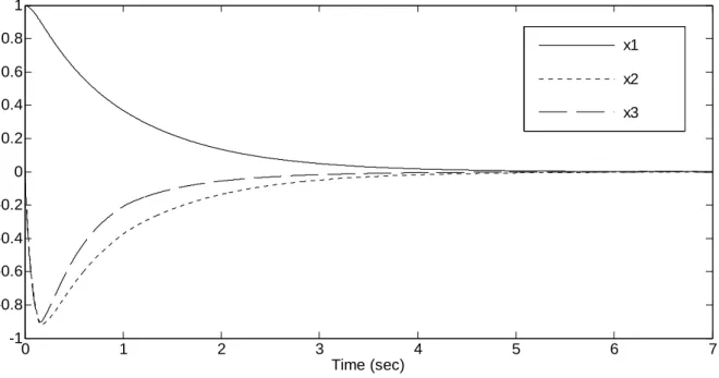
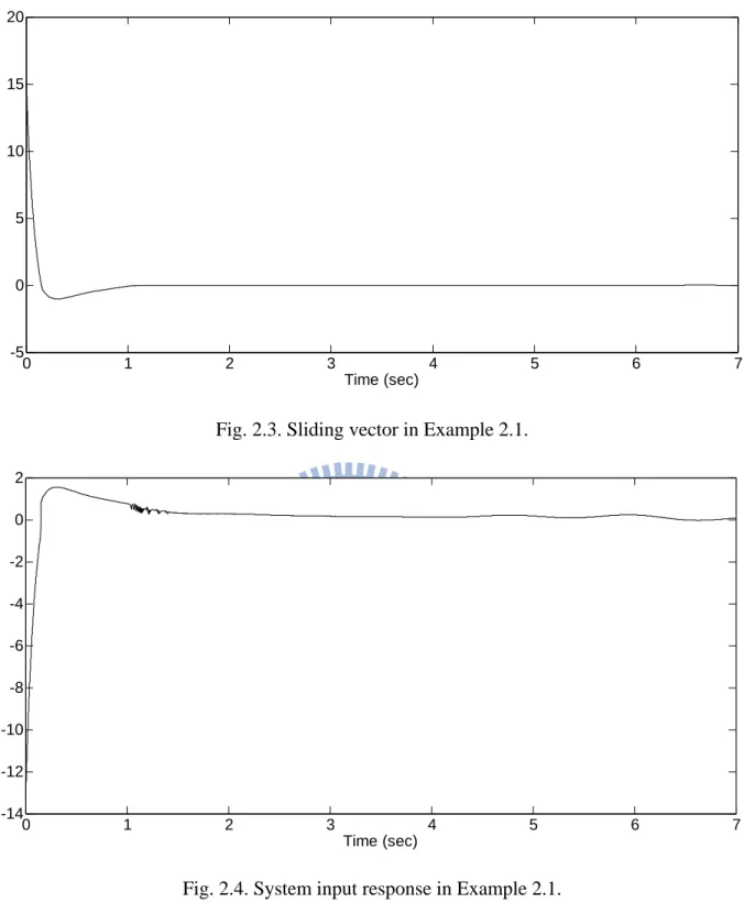
T, the simulation results are depicted in Fig. 2.1-2.4. The state and output responses are shown in Figs. 2.1 and 2.2 respectively, converging around zero successfully. Since (2.26) holds, all trajectories of system states in Fig. 2.1 converge to zero quadratically as the analysis of (2.33). Figure 2.3 showed the sliding vector and verified that the system entered into the sliding layer in a finite time. Matching the derivation of (2.36), the approaching behavior occurs after the sliding vector entering the local region around zero in Fig. 2.3. According to the control input shape in Fig. 2.4, the sliding mode controller has avoided the chattering phenomenon indeed due to the replacement of saturation function in the control input.

0 1 2 3 4 5 6 7 -1 -0.8 -0.6 -0.4 -0.2 0 0.2 0.4 0.6 0.8 1 Time (sec) x1 x2 x3

Fig. 2.1. System state responses in Example 2.1.

0 1 2 3 4 5 6 7 -3 -2 -1 0 1 2 3 4 5 Time (sec) y1 y2

0 1 2 3 4 5 6 7 -5 0 5 10 15 20 Time (sec)

Fig. 2.3. Sliding vector in Example 2.1.

0 1 2 3 4 5 6 7 -14 -12 -10 -8 -6 -4 -2 0 2 Time (sec)

Fig. 2.4. System input response in Example 2.1.

2.3 Summary

This chapter has introduced a series of coordinate transformations, the sliding vector design method, and the sliding mode controller design, demonstrating the feasibility by the numerical example. Output feedback sliding mode control method still possesses the robustness against matched disturbances as the state feedback sliding mode controller. The

designed controller can satisfy the approaching condition simply and improve the chattering phenomenon by the replacement of saturation function. Nevertheless, the static output feedback sliding vector has no ability locating eigenvalues of the system in the sliding mode arbitrary even though the system is controllable and observable. Besides the difficulty of designing the sliding vector, the output feedback sliding mode controller design suffered a structural constraint as a synthesis problem. Even though the synthesis constraint was satisfied, the designed controller guaranteed the local stability quadratically only rather than the global one.

For improving drawbacks of the static output feedback sliding mode controller mentioned above, next chapter will propose a dynamic output feedback sliding mode controller based on an integral sliding surface. The dynamic controller design can avoid the synthesis problem and assure the global stability using an adaptive law to estimate one of the controller parameters. The integral sliding surface and controller parameters will be offered by solutions to an algebraic Riccati equation.

III OUTPUT FEEDBACK INTEGRAL SLIDING MODE

CONTROL

This chapter addresses the problem of designing an output feedback integral sliding mode control algorithm for linear MIMO systems with mismatched parameter uncertainties along with disturbances and matched nonlinear perturbations. Once the system is in the sliding mode, the proposed method of output-dependent integral sliding surface can robustly stabilize the closed-loop system and obtain the desired system performance. Two types of mismatched disturbances are considered and their effects in the sliding mode are explored. By introducing an additional dynamics into the controller design, the developed control law can guarantee that the system globally reaches to the stable sliding surface in a finite time. Finally, the feasibility of the proposed method is illustrated by numerical examples.

The system and the problem formulation are described in section 3.1. Section 3.2 presents the design of output-dependent integral sliding surface using the static output feedback technique and develops the controller design. The effectiveness of the proposed controller is illustrated in section 3.3 with numerical examples. A concluding summary is given in section 3.4.

3.1 Problem Formulation

Consider a continuous-time uncertain system described in the state space form as

 



 



 



 







 

 

 

, , t t t t t t t t        x A D H x B u f x u Ed y Cx  (3.1)

where x

 

t n is the system state vector, y

 

t l is the system output vector,

 

_{t } m

u  is the control input vector, and d

 

t p is the mismatched disturbance vector. The system matrices A, B, C, D, E and H are known matrices and have appropriate dimensions with l m . Notice that E belongs to the columns of Bn n m   which span

the null space of B [10]. The function T f x u



, ,t



m is a time-varying vector in which it represents the lump sum of matched nonlinearities and/or uncertainties. In addition, 

 

t is an unknown matrix satisfying T

   

t  t  I . Although system (3.1) contains the mismatched disturbance, we design in this chapter an output-dependent integral sliding surface so that the proposed method can guarantee robust stability [55] of the closed-loop system once the system is in the sliding mode. A control law using output information and an additional dynamics is then designed to make the system globally satisfy the reaching and sliding condition [2]. Before introducing the proposed method, the following five assumptions are made throughout this chapter.

Assumption 3.1 The matched uncertain term is norm-bounded as



, , t



 a1 a2

 

t 

 

t

f x u x u (3.2)

where 0   , 1 a and 1 a are known positive constants. 2

Assumption 3.2 The mismatched disturbance is bounded as

 

t d

d (3.3)

where d  is a known constant. 0

Assumption 3.3 The pairs of



A B,



and



C A,



are stabilizable and detectable,

respectively.

Assumption 3.4 The triple



C A B, ,



is of minimum phase.

Assumption 3.5 Matrices B and C have full rank, and rank

 

CB rank

 

B m.

As for Assumption 3.1, it is different from that in other papers [2, 7-8, 15-17, 21] in which the matched uncertainty f x u



, , t



is bounded by a function of the system outputs. Yan et al. [60] have shown that the condition is quite restrictive. Our proposed control scheme can eliminate the limitation. Assumptions 3.2-3.5 are generally developed from the

conventional output feedback sliding mode control methods [2, 7-9, 15-21, 29].

3.2 Dynamic Output Feedback Sliding Mode Control

In this section, a design method of using the output-dependent integral sliding surface is proposed, in which robust stability of the closed-loop system can be guaranteed once the system is in the sliding mode. Seeking next to design the integral-type sliding surface for both matched and mismatched uncertain systems, Cao and Xu [22] developed a state-dependent integral sliding surface design in which the system is maintained on the sliding surface from the initial moment. However, the main problem related to the implementation of their method [22] is the requirement of the system states and their corresponding initial condition. In this work, we extend Cao and Xu’s method to the uncertain system with regard to which only the output information is obtainable. Applying H control analyzing technique, the existence condition of the sliding surface is determined by solving an algebraic Riccati equation which is involved with the original system parameters. In comparison with the other output feedback sliding mode controllers [15-18, 21, 23-26, 60], our proposed control law can obtain global robust stability and avoid the high gain phenomenon in the transient time. Moreover, our control algorithm does not need any observer structure to estimate the system states.

3.2.1 Integral sliding surface design

Design the output-dependent integral sliding surface as

     

₀t

 

t   t 

_

 d s CB y v (3.4) where

 



 



 

1 T  T _{m l}  _  

CB CB CB CB  , s , and the vector m v is designed m

later. Taking the derivative of s

 

t with respect to time and substituting (3.1) into it, we can obtain

   

t  



 

 

t



     

t  t  t 



, ,t

  

 

 

t

s CB C A D H x v u f x u CB CEd . (3.5)

 

t 



, ,t

      

 t  t  



 

 

t



   

t  

 

t

u f x u s v CB C A D H x CB CEd (3.6)

and then substitute it into (3.1) to obtain

 



 





 



 



 



 

 

 

 



1 1



 

1

 

 

 

n n t t t t t t t t t t t                 x I B CB C A D H x I B CB C Ed Bv Bs A D H x E d Bv Bs    (3.7) where A₁



I_nB CB

 

C A



, D₁



I_nB CB

 

C D



, and E₁ 



I_n B CB

 

C E



. Suppose that the system is in the sliding mode, s

 

t 0 for t t where ₁ t₁ is a finite 0 time. Then from (3.7) we obtain the system dynamics as

 

t 

_

1 1

 

t

_

 

t  1

 

t 

 

t

x A D H x E d Bv for t t . (3.8) ₁

Once the system is in the sliding mode, it follows from (3.8) that the robust stability problem of the closed-loop system becomes a standard output feedback controller design. As a result, the vector v

 

t is a variable in the designed integral sliding surface, playing a role to affect the behavior of the system in the sliding mode. For system (3.8), a robust static output feedback controller is to be designed with the control algorithm in the form [17, 53-54, 56]

 

t  

 

t  

 

t

v FCx Fy (3.9)

so that the closed-loop system x

 

t 



A₁BFC D₁

 

t H x



 

t is stable for all admissible uncertainties. Before introducing the main result, we have the following lemmas.

Lemma 3.1 If Assumptions 3.3 to 3.5 hold, then the pairs



A B₁,



and



C A, ₁



are

stabilizable and detectable, respectively.

Proof: Since state feedback control methods cannot change the controllability, from

 

1

  

A A B CB CA , we can conclude that the pair



A B₁,



is stabilizable. From

 

1 n n n m s s                  _ _   I 0 I A B I A B